On the Realized Risk of Foreign Exchange Rates: A Fractal Perspective

Abstract

While well-established literature argues that realized variances are close to a lognormal distribution, this study follows Benoit Mandelbrot by taking a fractal perspective. Using power laws to model realized foreign exchange rate variances, our findings indicate that power laws offer an alternative to the lognormal in terms of goodness-of-fit tests. Further, our analysis shows that estimated power law exponents for seven out of nine realized FX variances are $\widehat{\alpha }<3$, which indicates that the variance of realized variance is statistically undefined. We conclude that the foreign exchange rate market is far riskier than earlier believed. By implication, documented research in an enormous body of literature that draws conclusions from variance analyses stands on shaky grounds.

“There are strong pragmatic reasons to begin the study of economic distributions and time series by those that satisfy the law of Pareto.”

(Benoit Mandelbrot, mathematician known for the Theory of Roughness and Fractals)

1. Introduction

Uncertainty in the foreign exchange rate (FX) market has been the subject of intense study in the academic literature. This attention is not surprising in view of the fact that FX market capitalization is considerably larger than that in any other financial market. In 2022, the daily turnover of the global foreign exchange market with 39 different currencies reached 7.5 trillion per day.1 Previous studies investigating FX risk have employed GARCH-type models (e.g., Jorion 1995; Baillie and Bollerslev 1991; Bollerslev and Melvin 1994).2 Despite the widespread usage of GARCH-type models to analyze uncertainty in the FX market, work by Andersen et al. (2003) and Andersen et al. (2004) showed that simple reduced-form time series models for realized volatility (RV) outperform commonly-used GARCH-type models for forecasting future volatility. Unfortunately, many researchers incorporating RV to model FX risk have found there is a problem with realized variances (e.g., Wang and Yang 2009; Corsi 2004; Andersen et al. 2005; Bubák et al. 2011; Corsi et al. 2008). Specifically, Taleb (2020, p. 33) observed that, because the empirical distribution misrepresents the expected realizations in the tails, past data are not useful for predicting future maximums.

Power law functions offer a remedy to the aforementioned problem because the tail exponent of a power law function captures via extrapolation low-probability deviations not seen in the data. Taleb emphasized that such deviations play a disproportionately large share in determining the mean of the distribution. In advocating the usage of power law functions in empirical finance research, he argued that “There are a lot of theories on why things should be power laws, as sort of exceptions to the way things work probabilistically. But it seems that the opposite idea is never presented: power laws should be the norm, and the Gaussian a special case …” Taleb (2020, p. 91).

This study uses power laws to explore the risk of foreign exchange rates in terms of weekly realized variances. Based on a sample of daily prices from 16 May 2006, to 29 December 2023, we compute weekly variances by summing the squared returns over five business days for each currency pair, leaving us with 920 weekly observations. Subsequently, as proposed by Clauset et al. (2009), we employ the maximum likelihood estimation approach to estimate power law exponents. Furthermore, we use the goodness-of-fit (GoF) test derived by these authors for testing various distributions, including lognormal, exponential, and power law. If the p-value for the power law model is higher than for the other competing distributions, the power law model is favored.

Our study contributes to the literature in several ways. First, it extends previous studies on power laws in financial economics. Calvet and Fisher (2004) and Lux et al. (2014) found that power law models usually outperform GARCH models in terms of forecasting future volatility. Some recent studies by Grobys (2021, 2023) used power law functions to model realized variances for foreign exchange rates, the S&P 500, and some commodities. Also, Grobys et al. (2021) employed power law functions to model the realized volatilities of some cryptocurrencies. The commonality among these studies is that the power law null model cannot be rejected for virtually all realized asset market variances. The study by Grobys (2023) found that estimated power law exponents vary between $\widehat{\alpha }=2.2515$ and $\widehat{\alpha }=2.780,$ which indicates that the variance of daily realized FX variance does not exist. Further, using an application of Bayes’ rule, he documented that, for the vast majority of realized FX rate variances, the lognormal performs worse in predicting likelihoods for the arrivals of extreme events; hence, the power law model should be favored. The present research adds to this literature by (a) using lower-frequented data; and (b) employing GoF tests to compare various potential distributions. The application of Bayes’ rule in Grobys (2023) only provides evidence on the distribution that is associated with the most extreme events. Our approach is complementary in that we explicitly perform statistical tests using probability density functions. Furthermore, Mandelbrot (2008) argued that power law behavior is manifested in invariance of the power law exponent as time frequency changes. Hence, if realized FX variance exhibits fractal-like properties, we would expect that our estimates derived from weekly data should be close to the estimates documented for daily data. Moreover, due to the high rate of false discoveries in financial economics, Hou et al. (2020), Serra-Garcia and Gneezy (2021), and others have recommended scientific replications of reported research. Since we model realized foreign exchange rate variances using a different but related methodology to Grobys (2023), consistent with Hamermesh (2007), we provide replication findings to better understand the fractal-like nature of FX variances.

Relevant to our study, well-established literature has found that the distribution of realized volatility is typically very close to a lognormal distribution (e.g., Andersen et al. 2001a, 2001b; 2003). Renò and Rizza (2003) examined the unconditional volatility distribution of the Italian futures market. They concluded that the standard assumption of lognormal unconditional volatility is rejected and that a much better description is the Pareto distribution. Hence, there is no consensus in the literature on this issue. Is realized variance a lognormal distribution or closer to a power law? To our knowledge, no previous studies explicitly test power laws against other competing distributions to clarify this issue.

Using weekly realized FX variances over the sample from 16 May 2006, to 29 December 2023, our findings indicate that estimated power law exponents vary between $\widehat{\alpha }=2.4834$ and $\widehat{\alpha }=3.5968$. Strikingly, six out of nine realized FX variances have $\widehat{\alpha }<3$, which indicates that the variance of realized variance is statistically undefined. Since realized FX variances show fractal-like behavior, our results are in line with Grobys (2023) and corroborate Mandelbrot’s (2008) arguments. Furthermore, using a significance level of 5%, GoF tests suggest that we cannot reject the power law model for seven out of nine realized FX variances as indicated by p-values > 5%. Interestingly, GoF tests suggest that the lognormal model cannot be rejected for eight out of nine realized FX variances. However, a comparison of the p-values shows that, for five realized FX variances, the p-values for the power law models are substantially higher than the corresponding p-values derived from the lognormal model. Since our findings are consistent with Grobys (2023), we conclude that power laws should be preferred for modeling realized FX risk.

The paper is organized as follows. The next section describes the data. Section 3 discusses the methodology. The last section provides discussion and concluding remarks.

2. Data

The data consist of daily observations downloaded from the global financial website investing.com (accessed on 1 January 2023) for Group of Ten (G10) currency pairs, including AUD/USD, EUR/USD, GBP/USD, NOK/USD, NZD/USD, USD/CAD, USD/CHF, USD/JPY, and USD/SEK. To ensure comparability with earlier documented results, we utilize a sample that is similar to earlier research. Retrieving data from yahoo.com, Grobys (2023) documented that data for the AUD/USD exchange rate are only publicly available from 16 May 2006. Therefore, our study employs data from 16 May 2006, to 29 December 2023. The analysis is restricted to daily data, wherein all FX rates are quoted on the same day, which results in 4599 daily observations. The daily return is computed as follows:

$${RET}_{i,t}=100\ast \frac{\left(P_{i,t+1}-P_{i,t}\right)}{P_{i,t}},$$

(1)

where ${RET}_{i,t}$ denotes the return of FX i at time t and $P_{i,t}$ denotes the corresponding daily price. The weekly realized variance (WRV) of G10 currency pairs is computed as the sum of the squared returns over five business days for each currency pairs:

$${WRV}_{i,j}={\sigma }_{i,j}^2={\sum }_{t\in j}{\left({RET}_{i,t}\right)}^2,$$

where j indicates the week and $t\in j$ indicates the corresponding trading days in the respective week.

Table 1. Summary statistics for the weekly realized variances of G10 currencies.

	AUD/USD	EUR/USD	GBP/USD	NOK/USD	NZD/USD	USD/CAD	USD/CHF	USD/JPY	USD/SEK
Mean	3.3170	1.6138	1.8063	3.2683	3.2357	1.5839	2.1195	1.9851	2.9710
Median	1.6427	1.0225	1.1017	1.9579	1.8758	0.9303	1.0874	1.0876	1.7309
Std.Dev.	8.7209	1.9674	3.3995	4.8487	4.8140	2.3482	9.2697	3.1163	4.0658
Kurtosis	187.8401	27.0404	289.4048	90.3521	91.2411	64.0870	618.1327	57.6324	25.8182
Skewness	12.3553	4.1499	13.9099	7.5595	7.2678	6.5452	23.5305	5.7512	4.3111
Minimum	0.0676	0.0333	0.0427	0.0398	0.0641	0.0230	0.0081	0.0155	0.0870
Maximum	161.8294	21.9666	78.6839	77.0604	82.8622	31.4039	255.0862	47.5975	39.5884
Obs	920	920	920	920	920	920	920	920	920

reports the descriptive statistics of weekly realized variances for all nine currency pairs. The maximum and minimum values reveal a wide range of realized variances across most of the currency pairs, with USD/CHF showing the largest and EUR/USD the smallest fluctuations. The standard deviations represent the volatility of the realized FX rates variances, with USD/CHF and EUR/USD exhibiting the highest and lowest values, respectively. All currency pairs have high kurtosis due to the presence of fat tails in the distribution of weekly realized variances. Furthermore, among all FX weekly realized variances, skewness is most pronounced for realized USD/CHF variance.

This table provides the descriptive statistics of the weekly realized variances for G10 currency pairs, including EUR/USD, AUD/USD, GBP/USD, NOK/USD, NZD/USD, USD/CAD, USD/CHF, USD/JPY, and USD/SEK. The weekly realized variance is computed using daily data from investing.com, spanning from 16 May 2006, to 29 December 2023, and includes 920 observations.

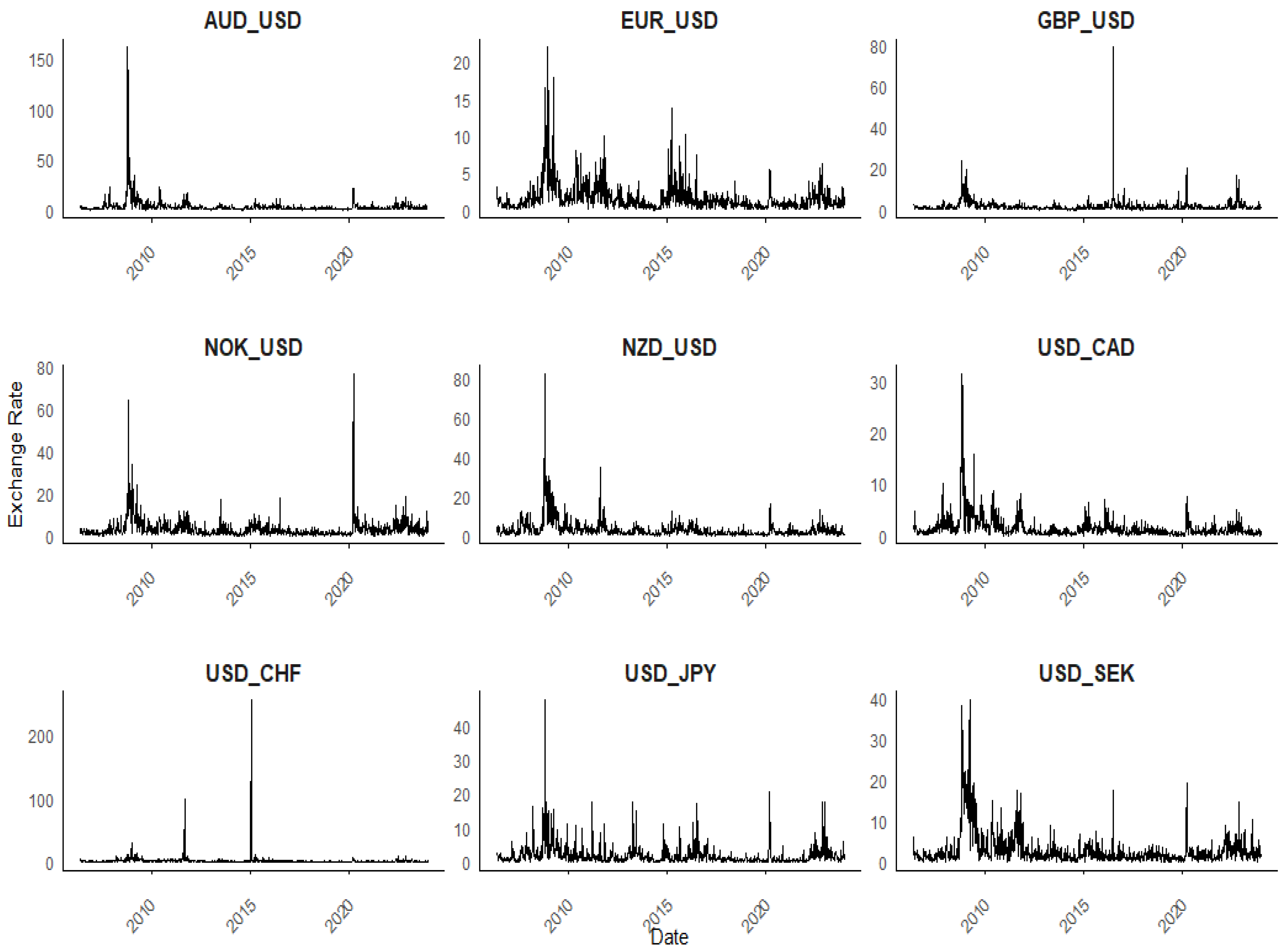
Next, we conduct a visual analysis of the time series plots for each currency pair’s realized variance to better understand how they evolved over time. Figure 1 provides a time series plot of the realized FX variances of various currency pairs. The key feature that stands out in these plots is that there are more extreme values or sudden shifts (spikes) than would be expected under normal or lognormal distributions. Some realized FX variances, such as the AUD/USD realized variance and the GBP/USD realized variance, have fewer spikes overall compared to other data series such as the EUR/USD realized variance and USD/JPY realized variance. These results suggest that the former pairs experienced fewer periods of extreme volatility during the sample period. The distribution of spikes over time is not uniform. Some realized FX variances, like the USD/CAD realized variance, show a concentration of extreme events around certain years. For example, there is a noticeable spike around 2008–2009 for the AUD/USD realized variance, which coincides with the global financial crisis. During this period, the Australian dollar had significant volatility arising from its close ties with global commodity prices and risk sentiment. Multiple spikes can be observed for the EUR/USD realized variance from 2010 to 2012, which is likely associated with the European sovereign debt crisis. The sharp spike for the GBP/USD realized variance around 2016 appears to be related to the Brexit referendum in which the United Kingdom voted to leave the European Union. This event caused significant uncertainty and led to a sharp depreciation of the British pound against the US dollar. Additionally, there is some asymmetry in the direction of the spikes. For example, the NOK/USD realized variance and the NZD/USD realized variance show shifts both upward and downward, whereas the EUR/USD realized variance shows predominantly upward shifts. These patterns indicate that certain currencies are more prone to strengthening or weakening against the US dollar under specific conditions. In sum, the presence of fat tails in the graphs indicates that events thought to be very rare may actually occur more frequently than expected. This finding has significant implications for financial risk management, as models based on normal or lognormal distributions may well underestimate the probability of extreme movements and thereby underestimate risk.

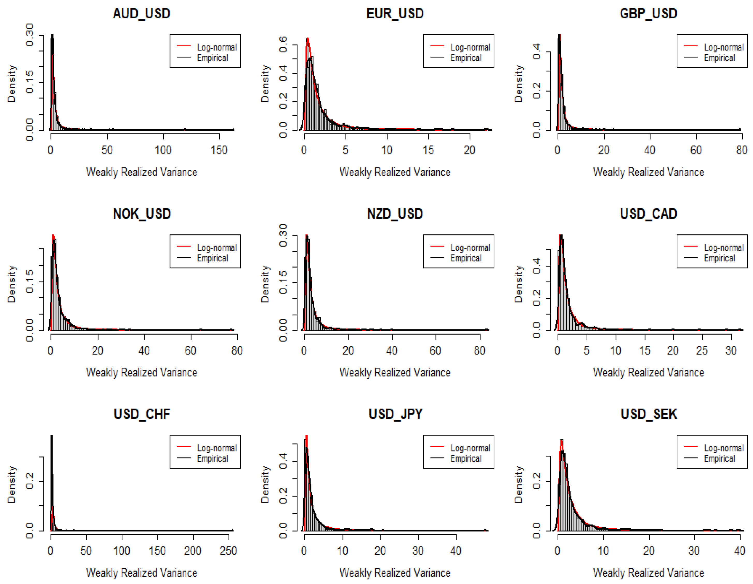
Figure 2 shows the difference between the theoretical lognormal distribution (red curve) and the distribution followed by each currency pair’s weekly realized variance (black curve). In some cases, especially for currency pairs such as the USD/CHF realized variance and the AUD/USD realized variance, the empirical distribution has a higher peak (kurtosis) and heavier tails as shown by the empirical line extending further along the x-axis than the lognormal line. The presence of heavy tails in the empirical distribution indicates that extreme events—for instance, arising from financial crises, political events, or sudden economic shifts, etc.—leading to large variances in exchange rates are not as rare as the normal or lognormal distribution would suggest. As already mentioned, financial risk management and derivative pricing often wrongly assume lognormality in their models. Additionally, the realized variances of different currency pairs show different levels of variance and different fits to the lognormal distribution. For instance, the EUR/USD realized variance and GBP/USD realized variance have a lower spread, whereas the USD/CHF realized variance shows a much wider spread. These patterns reflect different levels of market volatility and risk associated with each underlying currency pair. Overall, the plots suggest that lognormal distribution is not an adequate model for the distribution of weekly realized variances of these currency pairs.

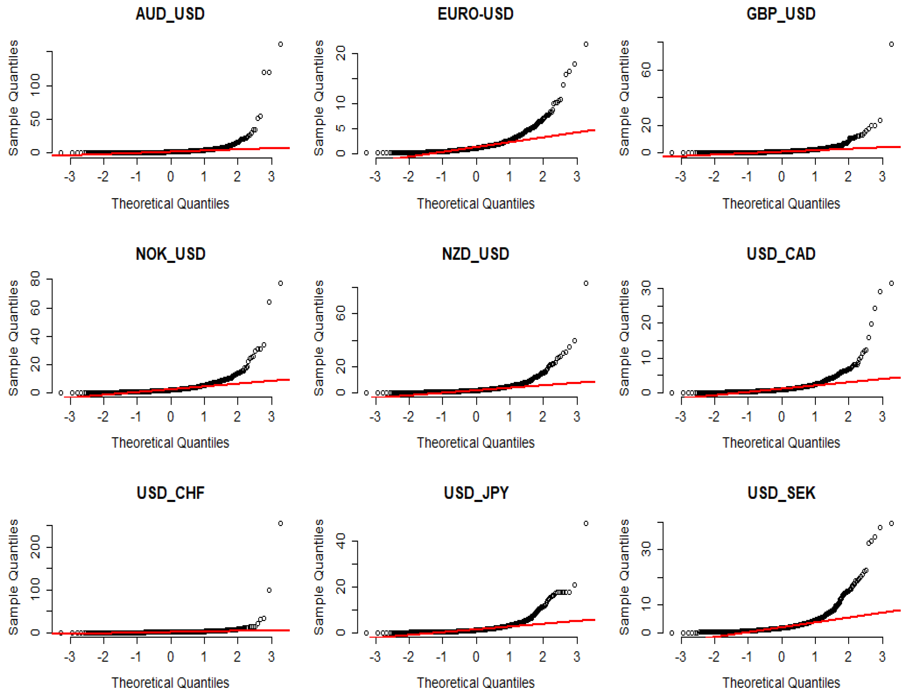
Figure 3 shows Lognormal quantile–quantile (QQ) plots. They offer a graphical tool to evaluate if a dataset follows lognormal distribution. It is evident that, even though all of the weekly realized variances of the currency pairs show a central tendency that follows a lognormal distribution, they exhibit heavy-tailed behavior as illustrated by the deviations from the theoretical line in the tails. This pattern again is indicative of a fat-tailed distribution, implying a higher frequency of extreme events than what would be expected by a lognormal distribution.

Below are time series graphs of monthly realized variance for weekly realized variances of G10 currency pairs, including EUR/USD, AUD/USD, GBP/USD, NOK/USD, NZD/USD, USD/CAD, USD/CHF, USD/JPY, and USD/SEK, using data from 16 May 2006, to 29 December 2023.

This figure illustrates theoretical lognormal distribution (red curve) versus the empirical distribution (black curve) for the weekly realized variances of G10 currencies, accounting for the following currencies: AUD/USD, EUR/USD, GBP/USD, NOK/USD, NZD/USD, USD/CAD, USD/CHF, USD/JPY, and USD/SEK. The sample is from 16 May 2006, to 29 December 2023.

The figure illustrates the theoretical log-normal quantile (red line) versus the quantile of weekly realized variance for G10 currency pairs including AUD/USD, EUR/USD, GBP/USD, NOK/USD, NZD/USD, USD/CAD, USD/CHF, USD/JPY, and USD/SEK. The sample is from 16 May 2006 to 29 December 2023.

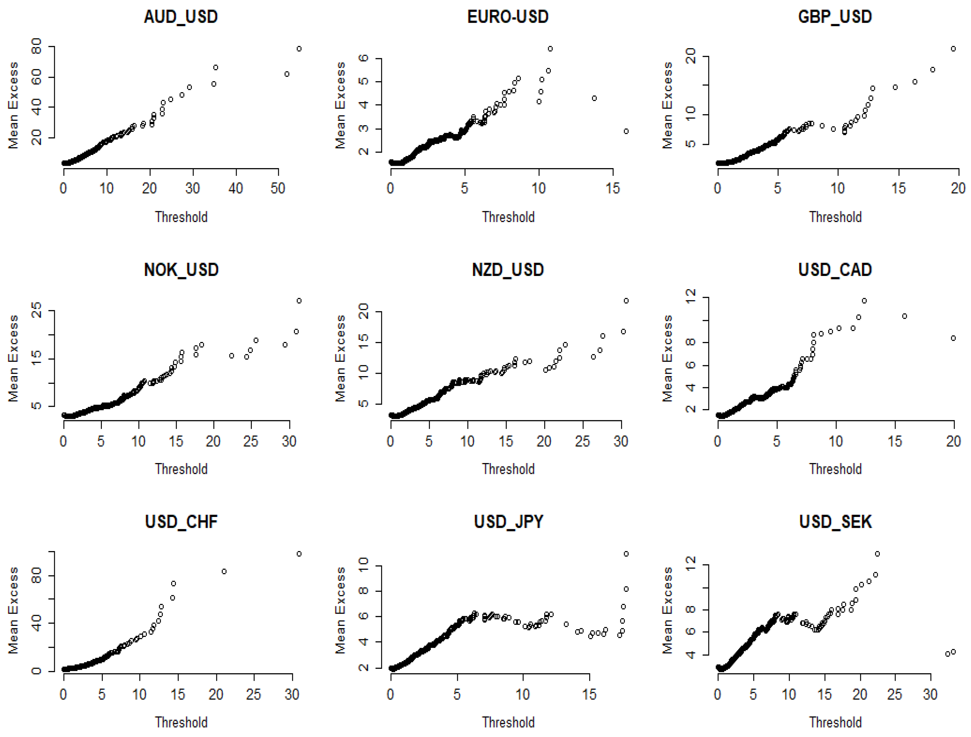
In Figure 4, we employ the mean excess function (ME) plot to evaluate potential power law behaviors for our data. For a given threshold $u$, the mean excess of a random variable $X$ is defined as:

$$E\left(X-u|X>u\right).$$

(2)

The presence of a linear upward trend in the ME plot points is consonant with power law behavior, where the slope of the line is directly related to the tail index parameter $\alpha$. A greater value for $\alpha$ typically denotes a steeper slope on the ME plot. As depicted in Figure 4, the linear trend in the initial part of the plots is suggestive of a distribution with heavy tails, such as a power law distribution.

This figure displays the sorted data on the x-axis against the corresponding values of the mean excess function of weekly realized variances for G10 currency pairs, including AUD/USD, EUR/USD, GBP/USD, NOK/USD, NZD/USD, USD/CAD, USD/CHF, USD/JPY, and USD/SEK, using the whole dataset from 16 May 2006, to 29 December 2023. For a given threshold $u$ of a random variable $X$, the mean excess is defined as $E\left(X-u|X>u\right).$

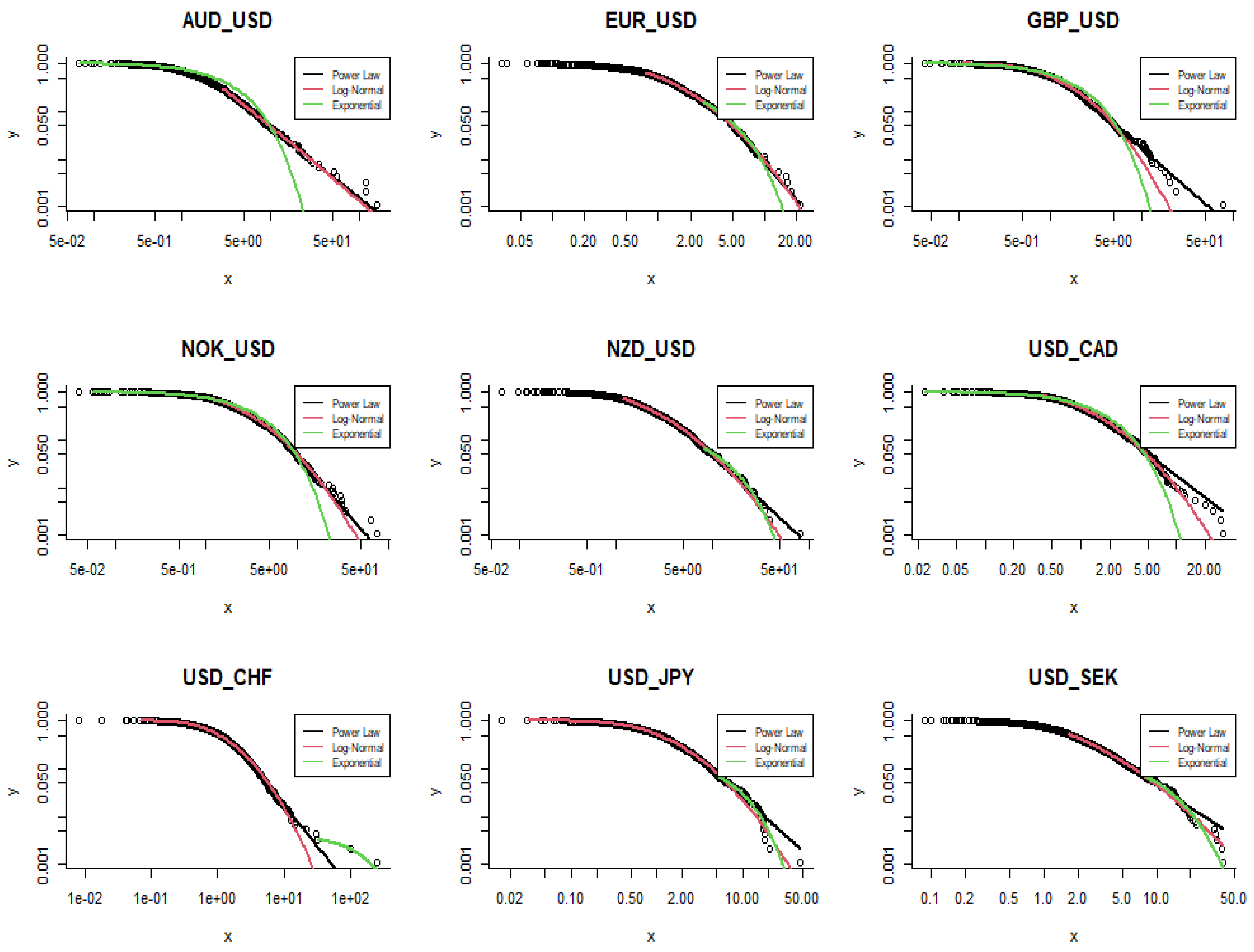
Finally, we plot in Figure 5 the cumulative distribution function (CDF) of weekly realized variances for G10 currency pairs. Here, we compare the empirical CDF of each currency pair’s realized variance with the power law (black), lognormal (red), and exponential (green) distributions. According to Figure 5, the power law and lognormal distributions align closely for AUD/USD and EUR/USD. However, power law provides a superior fit for GBP/USD, NOK/USD, USD/CAD, and USD/CHF, whereas exponential distribution is most suitable for USD/JPY and USD/SEK.

This figure illustrates the cumulative density functions for the weekly realized variances of G10 currency pairs, including AUD/USD, EUR/USD, GBP/USD, NOK/USD, NZD/USD, USD/CAD, USD/CHF, USD/JPY, and USD/SEK, using data from 16 May 2006, to 29 December 2023. The fitted power law (black line), lognormal (red line), and exponential (green line) distributions are also given.

3. Methodology

3.1. Estimating Power Law Exponents Using Maximum Likelihood Estimation

In line with Grobys (2021, 2023), we utilize the power law function to model the variances of foreign exchange rates as:

$$p\left(x\right)={Cx}^{-\alpha },$$

(3)

where $C={\left(\alpha -1\right)x}_{MIN}^{\alpha -1}$ with $\alpha \in \left\{{\mathbb{R}}_{+}\left|\alpha \right.>1\right\}$, $x=$ ${\sigma }_i^2$ denotes the respective realized weekly FX variance for currency pair i, provided $x\in \left\{{\mathbb{R}}_{+}\left|x_{MIN}\le x<\infty \right.\right\}$, $x_{MIN}$ is the minimum value of realized FX variance that is obtained by a power law process, and $\alpha$ is the magnitude of the specific tail exponent.3 The expected value of the realized weekly FX variance, given that $X>x_{MIN}$, is defined as $E\left[X\left|X>x_{MIN}\right.\right]$ and computed by:

$$E\left[X\left|X>x_{MIN}\right.\right]={\int }_{x_{MIN}}^{\infty }xp\left(x\right)dx=\frac{\left(\alpha -1\right)}{\left(\alpha -2\right)}{x}_{MIN}.$$

(4)

The second moment, which is the variance of the realized variance, given that $X>x_{MIN}$, is defined as $E\left[X^2\left|X>x_{MIN}\right.\right]$ and computed by:

$$E\left[X^2\left|{X>x}_{MIN}\right.\right]={\int }_{x_{MIN}}^{\infty }{x}^{2}p\left(x\right)dx=\frac{\left(\alpha -1\right)}{\left(\alpha -3\right)}{x}_{MIN}^2.$$

(5)

Finally, higher moments of order ‘k’ are computed as:

$$E\left[X^k\left|X>x_{MIN}\right.\right]=\frac{(\alpha -1)}{(\alpha -1-k)}{x}_{MIN}^k$$

(6)

Based on Equations (4) and (5), it is evident that the theoretical mean of realized variances is only defined for $\alpha >2$, whereas the variance of the realized variance requires $\alpha >3$.

Following White et al. (2008) and Clauset et al. (2009), who argued that maximum likelihood estimation (MLE) is the optimal method for calculating power law exponents, the tail exponents $\widehat{\alpha }$ are computed as follows:

$$\widehat{\alpha }=1+N{\left({\sum }_{i=1}^N\ln \left(\frac{x_i}{x_{MIN}}\right)\right)}^{-1},$$

(7)

where $\widehat{\alpha }$ denotes the MLE estimator, $N\le T$ is the number of observations greater than $x_{MIN}$, and the rest of notation is as earlier. According to Equation (7), the MLE estimator depends on the chosen $x_{MIN}$. Like Clauset et al. (2009), we select $x_{MIN}$ by minimizing the distance between the power law model and the empirical data defined as Kolmogorov–Smirnov distance (D) or maximum distance between the cumulative density functions (CDFs) of the data and the fitted model:

$$D={MAX}_{x\ge x_{MIN}}\left|S\left(x\right)-P\left(x\right)\right|$$

(8)

where $S\left(x\right)$ represents the cumulative distribution function (CDF) of the data for observations with values greater than or equal $x_{MIN}$, and $P\left(x\right)$ is the CDF for the power law model that provides the best fit to the data in the range of $x\ge x_{MIN}$. The estimate ${\widehat{x}}_{MIN}$ is determined as the value of $x_{MIN}$ that minimizes D. Moreover, the standard deviation for estimated power law exponents is defined as:

$$\sigma =\frac{\widehat{\alpha }-1}{\sqrt{N}}+O(\frac{1}{N}).$$

(9)

Summary statistics for the estimated power law exponents are presented in

Table 2. Estimated power law functions.

Distribution	$\widehat{\mathit{\alpha }}$	$\widehat{\mathit{\sigma }}$	${\mathit{x}}_{\mathit{M}\mathit{I}\mathit{N}}$	$\mathit{D}$	NPL	95% CI
AUD/USD	2.4834	0.0911	2.9452	0.0242	28.80%	[2.3048, 2.6620]
EUR/USD	3.5968	0.3126	4.3242	0.0497	7.50%	[2.9841, 4.2095]
GBP/USD	2.6704	0.1092	1.9530	0.0319	25.43%	[2.4563, 2.8844]
NOK/USD	3.1845	0.1978	6.1729	0.0389	13.26%	[2.7968, 3.5721]
NZD/USD	2.8648	0.1617	5.4697	0.0509	14.46%	[2.5479, 3.1818]
USD/CAD	2.5048	0.0869	1.4408	0.0535	32.61%	[2.3345, 2.6751]
USD/CHF	2.7312	0.1256	2.4059	0.0275	20.65%	[2.4851, 2.9774]
USD/JPY	2.5888	0.1276	3.0011	0.0485	16.85%	[2.3387, 2.8390]
USD/SEK	2.5553	0.1019	3.2868	0.0462	25.33%	[2.3556, 2.7550]

. The estimated tail exponent for the realized AUD/USD variance is $\widehat{\alpha }=2.4834$, with corresponding standard deviation $\widehat{\sigma }=0.0911$. It follows that $\widehat{\alpha }$ is 5.67 standard deviations below a hypothesized tail exponent corresponding to $\alpha =3$. Therefore, $\alpha$ for the realized AUD/USD variance is statistically significant $\alpha <3$ indicating that the variance of realized variance is statistically undefined. The same argument holds for the realized variances of USD/CAD, USD/GBP, USD/CHF, USD/JPY, and USD/SEK; however, the estimated tail exponent for the realized NZD/USD variance (e.g., $\widehat{\alpha }=2.8648$) is statistically not different from $\alpha =3$. Furthermore, we observe from Table 2 for the lower bounds of the 95% confidence intervals, $\alpha <3$ holds for all realized variance series, which provides further evidence that the infinite variance hypothesis cannot be rejected. Overall, we infer from these findings that the theoretical variances for the distributions of at least six out of nine realized FX variances are undefined, consistent with Grobys’ (2023) findings derived from daily data (viz., estimated power law exponents for daily range-based FX variances varied between $\widehat{\alpha }=2.2515$ and $\widehat{\alpha }=2.7807$).

This table reports the results of estimating power law exponents for weekly realized variances for G10 currencies, including AUD/USD, EUR/USD, GBP/USD, NOK/USD, NZD/USD, USD/CAD, USD/CHF, USD/JPY, and USD/SEK, using data from 16 May 2006, to 29 December 2023. The estimate $\widehat{\alpha }$ represents the estimated tail exponent and $\widehat{\sigma }$ is the estimated standard deviation. The lower threshold $x_{MIN}$ is estimated using the optimized Kolmogorov–Smirnov distance (D) distance as proposed by Clauset et al. (2009). The estimated $x_{MIN}$ is the value that corresponds to optimal distance D. N_PL denotes the percentage of sample observations governed by a power law process. The last column reports the 95% confidence interval (CI) intervals for the estimated power law exponents.

3.2. Testing the Power Law Model

According to Clauset et al. (2009), a tail exponent within the interval $2<\alpha <3$ does not necessarily indicate that the power law is a plausible fit to the data. Therefore, we need to verify whether the observed dataset genuinely adheres to a power law distribution. This test employs the Kolmogorov–Smirnov distance (D) as outlined in Equation (8). The objective is to determine whether the empirical data and synthetic data generated from the power law distribution, with specific $x_{MIN}$ and $\alpha$ values, originate from the same distribution. The null hypothesis for the goodness-of-fit test hypothesizes that the empirical data and the synthetic data generated from the power law distribution, with specified $x_{MIN}$ and $\alpha$ values, share the same distribution. If so, power law distribution is a plausible fit for the empirical data. Conversely, the alternative hypothesis posits that the empirical data and the synthetic data do not originate from the same distribution, which indicates that power law distribution is not a suitable fit for the empirical data. In this case, alternative distribution models should be explored to better characterize the underlying data distribution.

To implement this analysis, we generate large synthetic datasets followed by the power law distribution utilizing the estimated parameters $x_{MIN}$ and $\alpha$ derived from the previous section for each FX currency variances. Specifically, we compute the p-value of this test by fraction $\#(D_S>D)/K$, where $D_S$ represents the estimated Kolmogorov–Smirnov distance for a synthetic dataset with specified $x_{MIN}$ and $\alpha$ values mirroring those estimated for the original FX variances, D denotes the estimated Kolmogorov–Smirnov distance for the original dataset, and K is the number of synthetic datasets generated for testing purposes.

We set the significance level at 5%, which means that we do not reject the power law model if $\#\frac{D_S>D}{K}>0.05$. This test aims to determine whether the empirical data and the generated dataset share the same distribution. We use K = 500 synthetic data series to compute the p-values for the goodness-of-fit tests. The second column of

Table 3. Goodness-of-fit test.

	Power Law	Lognormal	Exponential
EUR/USD	0.96	0.05	0.00
AUD/USD	0.76	0.40	0.08
GBP/USD	0.64	0.38	0.14
NOK/USD	0.86	0.60	0.00
NZD/USD	0.30	0.90	0.10
USD/CAD	0.00	0.46	0.00
USD/CHF	0.98	0.26	0.44
USD/JPY	0.16	0.64	0.32
USD/SEK	0.04	0.86	0.40

reports the p-values corresponding to the null hypothesis of the power law model. It is evident that, for all realized FX variances, the p-values are above 5%, with the exception of USD/CAD and USD/SEK. These findings strongly support the notion that power laws are indeed plausible distributions for modeling realized FX variances.

This table reports the p-values from goodness-of-fit tests derived from the Kolmogorov–Smirnoff distance to examine if our empirical data and the generated data from the power law distribution with particular $x_{min}$ and $\alpha$ belong to the same distribution. The corresponding p-values are reported in the second column. The table gives the p-values for goodness-of-fit tests for exponential and lognormal distributions in the third and fourth columns, respectively. We use K = 500 synthetic data series to compute the p-values.

3.3. An Empirical Comparison of Distributions

Although our analysis in the previous section suggests that power law distributions provide a reasonable fit for realized FX variances, it should be noted that they may not be the optimal model, and other distributions could potentially offer a superior fit. Consequently, we focus on comparing two primary candidates—that is, the lognormal and exponential distributions against the power law to determine the appropriate fitting model for our data. It is important to note that prior studies have documented that realized volatility tends to follow a distribution that is nearly lognormal (e.g., Andersen et al. 2001a; 2001b, 2003). In our study, we investigate the suitability of the lognormal and exponential distributions for realized variance of G10 currency pairs. Employing a goodness-of-fit test similar to the one described by Clauset et al. in the previous section, we test the hypothesis that the lognormal (exponential) distribution can be considered a plausible fit. Thus, the lognormal (exponential) distribution is used as the null hypothesis against which the currency pair variances are tested at the 5 percent significance level as before. Columns 3 and 4 in Table 3 display the p-values of the goodness-of-fit test for lognormal and exponential distributions, respectively. The results in column 3 indicate that eight out of nine p-values exceed the significance level of 5%, implying that lognormal distribution is a plausible fit to the data, with the exception of the EUR/USD realized variance. In addition, the results in column 4 indicate that exponential distribution is at least a plausible fit for the realized variances of the following currency pairs: AUD/USD, GBP/USD, NZD/USD, USD/CHF, USD/JPY, and USD/SEK.

According to Clauset et al., using p-values for power law models alongside other potential alternative distributions (e.g., lognormal and exponential) allows us to construct a persuasive argument regarding the suitability of the power law model for all currency pairs. Specifically, they observed that a high p-value for the power law model in combination with lower p-values for other distributions supports ruling out alternative distributions. We find in Table 3 that power law models for the realized variances of EUR/USD, AUD/USD, GBP/USD, NOK/USD, and USD/CHF exhibit considerably higher p-values than the alternative distributions. Interestingly, Grobys (2023) employed an application of Bayes’ rule to examine the conditional probability that the underlying distribution is lognormally distributed, given that distribution-specific extreme events occurred. In doing so, he explored the cross-section of extreme events for daily realized range-based FX variances. His findings indicated that, when lognormal distribution is assumed and power law processes are equally likely, for six out of nine daily realized FX rate variances, the probability that the underlying distribution is lognormal given the arrival of the corresponding maximums is <25%. Even when it was assumed that lognormal distribution is 70% likely, for six out of nine daily realized FX rate variances, the probability that the underlying distribution is lognormal given the arrival of the corresponding maximums is <40%. Overall, Grobys (2023) concluded that, for the vast majority of realized FX rate variances, we can rule out a lognormal distribution as the corresponding underlying data-generating process for realized FX variances. The results of the present study in association with the results documented in Grobys (2023) provide evidence that power law models describe the distribution of realized FX variances more accurately. This inference is in line with Renò and Rizza (2003) but contradicts some well-established literature (Andersen et al. 2001a; 2001b; 2003).

3.4. Robustness Checks

Table A1. Sample-split analysis.

Panel A
Distribution	$\widehat{\mathit{\alpha }}$	$\widehat{\mathit{\sigma }}$	${\mathit{x}}_{\mathit{M}\mathit{I}\mathit{N}}$	$\mathit{D}$	NPL	95% CI
AUD/USD	2.4139	0.1666	6.2002	0.0545	15.65%	[2.0873, 2.7405]
EUR/USD	2.4325	0.0934	1.3364	0.0691	51.09%	[2.2493, 2.6156]
GBP/USD	2.5637	0.1196	1.4831	0.0416	37.17%	[2.3293, 2.7981]
NOK/USD	3.2158	0.2432	6.0219	0.0553	18.04%	[2.7391, 3.6926]
NZD/USD	2.4391	0.1085	3.4412	0.0582	38.26%	[2.2265, 2.6518]
USD/CAD	3.0643	0.2522	3.8276	0.0632	14.57%	[2.5700, 3.5586]
USD/CHF	2.7203	0.1640	2.9686	0.0462	23.91%	[2.3989, 3.0418]
USD/JPY	2.4901	0.1268	2.3796	0.0452	30.00%	[2.2415, 2.7387]
USD/SEK	2.3217	0.1058	3.2904	0.0736	33.91%	[2.1143, 2.5291]
Panel B
Distribution	$\widehat{\mathit{\alpha }}$	$\widehat{\mathit{\sigma }}$	${\mathit{x}}_{\mathit{M}\mathit{I}\mathit{N}}$	$\mathit{D}$	NPL	95% CI
AUD/USD	3.3773	0.2389	3.0557	0.0453	21.52%	[2.9090, 3.8456]
EUR/USD	2.7133	0.1342	1.1669	0.0481	35.43%	[2.4503, 2.9764]
GBP/USD	2.7723	0.1682	2.0690	0.0476	24.13%	[2.4426, 3.1020]
NOK/USD	2.8486	0.1591	3.1635	0.0389	29.34%	[2.5367, 3.1604]
NZD/USD	3.1287	0.2139	2.9721	0.0732	21.52%	[2.7094, 3.5481]
USD/CAD	3.0508	0.1772	1.2762	0.0650	29.13%	[2.7036, 3.3981]
USD/CHF	3.0085	0.1804	1.3947	0.0474	26.95%	[2.6550, 3.3620]
USD/JPY	2.8305	0.2538	3.2205	0.0528	11.30%	[2.3330, 3.3281]
USD/SEK	3.4147	0.2491	3.0119	0.0689	20.43%	[2.9266, 3.9029]

in the Appendix A reports the results from a sample-split analysis of estimating power law exponents. In this analysis, we divided the sample into two non-overlapping subsamples of equal length. Panel A of Table A1 reports the estimation results for the first subsample from 16 May 2006, to 3 March 2015, whereas Panel B documents the estimation results for the second subsample from 10 March 2015, to 29 December 2023. Each subsample includes 460 observations. From Table A1, it is evident that the point estimates ${\widehat{\alpha }}_{1i}$ and ${\widehat{\alpha }}_{2i}$ are fairly similar between the two subsamples. However, it is noteworthy that there are some differences between the two subsamples. For instance, subsample 1—covering the period up to 3 March 2015—includes the aftermath of the 2008 financial crisis and the European debt crisis, among other events. These severe economic events are likely to have influenced market volatility and, in turn, the behavior of currency variances. On the other hand, subsample 2 captures a different economic period, including the gradual recovery from previous crises, shifts in monetary policy across major economies, and the impact of the COVID-19 pandemic. Overall, from Panels A and B of Table A1 for the lower bounds of the 95% confidence intervals, it holds that α < 3 for all realized variance series, which is similar to our previously documented evidence.

4. Discussion and Concluding Remarks

The present study applied a fractal perspective to investigate the second moment of foreign exchange rates. We examined G10 currencies that account for approximately 70% of overall FX market capitalization. Instead of relying on parametric GARCH-type models, we utilized realized variances derived from daily price data. Realized variances are employed in MLE estimations, which provide reliable estimation even in the presence of extremely fat-tailed data. Well-established literature on realized volatility contends that the underlying distribution of realized asset uncertainty is close to normal (e.g., Andersen et al. 2001a; 2001b; 2003). Our findings contradict this view as power law models provide better data fits and more reliable probabilities for the arrivals of extreme events. We infer that the conventional lognormal distribution for modeling risk may severely underestimate tail risks.

Further findings indicated that the variance of variance does not exist for most of the foreign exchange rate variances under study. This evidence is in line with Grobys (2023), who fitted power laws to daily range-based FX variances. Mandelbrot (2008) argued that power law behavior is manifested in invariance of the power law exponent across time frequencies. In his seminal study on cotton price changes, Mandelbrot (1963) was the first to show that the power law exponent for cotton price changes does not change across various time frequency—a property suggesting fractal-like behavior. Consistent with his findings, weekly data on realized FX variances behave very similar to daily data.

An important implication of our empirical results is that standard statistical methodologies can lead to invalid inferences. In this regard, Fama (1963) observed that OLS regression assuming finite variances may not be appropriate in empirical analyses in financial economics due to infinite variances. Using a novel methodology that explicitly focuses on the statistical information residing in the tails, our findings suggested that the variances of the majority of exchange rate variance are infinite. As noted by Mandelbrot (2008), the reliance on traditional finance models gives a comforting impression of precision and competence:

“It is false confidence, of course. The problem lies at the roots of the standard model, in its assumption that the best way to think about stock markets is as a grand game of coin-tossing. If you are going to use probability to model financial markets, then you had better use the right kind of probability. Real markets are wild. Their price fluctuations can be hair-raising–far greater and more damaging than the mild variations of orthodox finance.” (Mandelbrot 2008, p. 105).

This study supports Mandelbrot’s (2008) viewpoint that price fluctuations in the currency market are wild—indeed so uncertain that the second moment of realized variances does not converge.

While we focused on G10 currencies in the FX market, future research is recommended to explore this issue in other financial markets, such as the market for cryptocurrencies which is exposed to greater risks than established financial markets. Also, it is possible that, as documented in Ibragimov et al. (2013), power law behavior could be more pronounced in emerging than advanced economies. Hence, future research is warranted to investigate this issue for emerging economies.

Finally, Gabaix and Ibragimov (2011) proposed various approaches for estimating the optimal tail exponent. Several studies have concluded that inferences based on the tail index using a maximum likelihood estimator suffer from shortcomings, including sensitivity to dependence and small sample sizes (e.g., Embrechts et al. 1997). Even though our sample consists of sufficient numbers of realized variance observations, dependency could exist in our data. We chose the MLE approach in line with Clauset et al. (2009) to (1) ensure that our results are comparable to previous studies and (2) implement goodness-of-fit tests to discriminate between competing distributions. However, following Gabaix and Ibragimov, future studies are encouraged to use the log–log rank size OLS regression approach rather than the MLE approach.

References

- Alexander, Carol O. 1995. Common volatility in the foreign exchange market. Applied Financial Economics 5: 1–10. [Google Scholar] [CrossRef]
- Andersen, Torben G., Tim Bollerslev, and Francis X. Diebold. 2005. Roughing It Up: Including Jump Components in the Measurement, Modelling and Forecasting of Return Volatility. NBER Working Paper No. 11775. Cambridge: National Bureau of Economic Research. [Google Scholar]
- Andersen, Torben G., Tim Bollerslev, and Nour Meddahi. 2004. Analytical evaluation of volatility forecasts. International Economic Review 45: 1079–110. [Google Scholar] [CrossRef]
- Andersen, Torben G., Tim Bollerslev, Francis X. Diebold, and Heiko Ebens. 2001a. The distribution of realized stock return volatility. Journal of Financial Economics 61: 43–76. [Google Scholar] [CrossRef]
- Andersen, Torben G., Tim Bollerslev, Francis X. Diebold, and Paul Labys. 2001b. The distribution of realized exchange rate volatility. Journal of the American Statistical Association 96: 42–55. [Google Scholar] [CrossRef]
- Andersen, Torben G., Tim Bollerslev, Francis X. Diebold, and Paul Labys. 2003. Modeling and forecasting realized volatility. Econometrica 71: 579–625. [Google Scholar] [CrossRef]
- Baillie, Richard T., and Tim Bollerslev. 1991. Intra-day and inter-market volatility in foreign exchange rates. Review of Economic Studies 58: 565–85. [Google Scholar] [CrossRef]
- Bauwens, Luc, Walid Ben Omrane, and Pierre Giot. 2005. News announcements, market activity and volatility in the euro/dollar foreign exchange market. Journal of International Money and Finance 24: 1108–25. [Google Scholar] [CrossRef]
- Bollerslev, Tim, and Michael Melvin. 1994. Bid—Ask spreads and volatility in the foreign exchange market: An empirical analysis. Journal of International Economics 36: 355–72. [Google Scholar] [CrossRef]
- Bubák, Vít, Evžen Kočenda, and Filip Žikeš. 2011. Volatility transmission in emerging European foreign exchange markets. Journal of Banking and Finance 35: 2829–41. [Google Scholar] [CrossRef]
- Calvet, Laurent E., and Adlai J. Fisher. 2004. Regime-switching and the estimation of multifractal processes. Journal of Financial Econometrics 2: 44–83. [Google Scholar] [CrossRef]
- Clauset, Aaron, Cosma Rohilla Shalizi, and Mark E. J. Newman. 2009. Power law distributions in empirical data. SIAM Review 51: 661–703. [Google Scholar] [CrossRef]
- Corsi, Fulvio. 2004. A Simple Long Memory Model of Realized Volatility. Working Paper. Lugano: Institute of Finance, University of Lugano. [Google Scholar]
- Corsi, Fulvio, Stefan Mittnik, Christian Pigorsch, and Uta Pigorsch. 2008. The volatility of realized volatility. Econometric Reviews 27: 46–78. [Google Scholar] [CrossRef]
- Embrechts, Paul, Claudia Klüppelberg, and Thomas Mikosch. 1997. Modelling Extremal Events for Insurance and Finance. New York: Springer. [Google Scholar]
- Fama, Eugene F. 1963. Mandelbrot and the stable Paretian hypothesis. Journal of Business 36: 420–29. [Google Scholar] [CrossRef]
- Gabaix, Xavier, and Rustam Ibragimov. 2011. Rank—1/2: A simple way to improve the OLS estimation of tail exponents. Journal of Business and Economic Statistics 29: 24–39. [Google Scholar] [CrossRef]
- Grobys, Klaus. 2021. What do we know about the second moment of financial markets? International Review of Financial Analysis 78: 101891. [Google Scholar] [CrossRef]
- Grobys, Klaus. 2023. Correlation versus co-fractality: Evidence from foreign-exchange-rate variances. International Review of Financial Analysis 86: 102531. [Google Scholar] [CrossRef]
- Grobys, Klaus, James W. Kolari, and Niranjan Sapkota. 2021. On the stability of stablecoins. Journal of Empirical Finance 64: 207–23. [Google Scholar] [CrossRef]
- Hamermesh, Daniel S. 2007. Viewpoint: Replication in economics. Canadian Journal of Economics 40: 715–33. [Google Scholar] [CrossRef]
- Hou, Kewei, Chen Xue, and Lu Zhang. 2020. Replicating anomalies. Review of Financial Studies 33: 2019–133. [Google Scholar] [CrossRef]
- Ibragimov, Marat, Rustam Ibragimov, and Paul Kattuman. 2013. Emerging markets and heavy tails. Journal of Banking and Finance 37: 2546–59. [Google Scholar] [CrossRef]
- Jorion, Philippe. 1995. Predicting volatility in the foreign exchange market. Journal of Finance 50: 507–28. [Google Scholar] [CrossRef]
- Lux, Thomas, Leonardo Morales-Arias, and Cristina Sattarhoff. 2014. A Markov-switching multifractal approach to forecasting realized volatility. Journal of Forecasting 33: 532–41. [Google Scholar] [CrossRef]
- Mandelbrot, Benoit B. 1963. The variation of certain speculative prices. Journal of Business 36: 394–419. [Google Scholar] [CrossRef]
- Mandelbrot, Benoit B. 2008. The (Mis)behavior of Markets. A Fractal View of Risk, Ruin and Reward. London: Profile Books. [Google Scholar]
- Renò, Roberto, and Rosario Rizza. 2003. Is volatility lognormal? Evidence from Italian futures. Physica A: Statistical Mechanics and Its Applications 322: 620–28. [Google Scholar] [CrossRef]
- Serra-Garcia, Marta, and Uri Gneezy. 2021. Nonreplicable publications are cited more than replicable ones. Science Advances 7: 1705. [Google Scholar] [CrossRef]
- Taleb, Nassim Nicholas. 2020. Statistical Consequences of Fat Tails: Real World Preasymptotics, Epistemology, and Applications. Papers and Commentary, STEM. Cambridge: Academic Press. [Google Scholar]
- Wang, Jianxin, and Minxian Yang. 2009. Asymmetric volatility in the foreign exchange markets. Journal of International Financial Markets, Institutions and Money 19: 597–615. [Google Scholar] [CrossRef]
- White, Ethan P., Brian J. Enquist, and Jessica L. Green. 2008. On estimating the exponent of power law frequency distributions. Ecology 89: 905–12. [Google Scholar] [CrossRef]
Figure 1.
Time series plot.
Figure 2.
Histogram plot.
Figure 3.
Lognormal QQ plot.
Figure 4.
Mean excess plot.
Figure 5.
Distribution comparison.