
Impact of the Environmental, Social, and Governance Rating on the Cost of Capital: Evidence from the S&P 500


International School of Finance (ISF), Nuertingen-Geislingen University, Sigmaringer Straße 25, 72622 Nuertingen, Germany
*
Author to whom correspondence should be addressed.
J. Risk Financial Manag. 2024, 17(3), 91; https://doi.org/10.3390/jrfm17030091
Submission received: 16 January 2024
/
Revised: 8 February 2024
/
Accepted: 12 February 2024
/
Published: 20 February 2024
(This article belongs to the Section Business and Entrepreneurship)
Abstract
:We use the S&P 500 to investigate whether companies with a good ESG score benefit from a lower cost of capital. Using Bloomberg’s financial data and MSCI’s ESG score for 498 companies, we calculated the measures of descriptive statistics, finding that companies with better ESG ratings enjoy both a lower cost of equity and a lower cost of debt. However, their WACC shows no improvement with a higher ESG score. Companies with a poor ESG rating have a lower WACC due to the higher proportion of debt capital, coupled with a higher cost of debt, compared to the cost of equity capital. Calculating the Pearson correlation coefficient, we found a slightly negative linear relationship between the ESG score and the beta factor, and between the ESG score and the cost of debt. No linear relationship was found between the WACC and the ESG score. Finally, linear regression analysis shows a negative and significant effect of the ESG score on the root beta factor. This research indicates that companies with better ESG scores benefit from lower cost of equity and debt. Our results may encourage companies to operate more sustainably to reduce their cost of capital.
1. Introduction
The Global Risks Report 2022, published by the World Economic Forum in 2022, makes it clear that in the long term, environmental risks pose the greatest threat to people and the environment today. This finding means that sustainability issues could become increasingly relevant in the future. Consequently, companies that do not operate sustainably will suffer disadvantages. The first signs of this can already be seen in the capital market. Some large, institutional investors already prefer to invest in companies that act sustainably and fulfill certain ESG criteria (PricewaterhouseCoopers International 2022). According to Bloomberg Intelligence (2021), ESG assets were able to generate an annual increase in volume of 30% in the period from 2016 to 2020. These assets are forecast to grow 15% annually in the future, meaning that USD 53 trillion is expected to be invested in ESG assets by 2025. From a capital market perspective, the relationship between a firm’s ESG assets and its cost of capital plays an important role. Cost of capital is used in determining the value of any asset, including the value of a company. If sustainable companies face lower ESG risk, they should benefit from lower capital costs, which in turn has a positive impact on cash flow and company value.
2. Literature Review and Research Question Development
2.1. Defining Corporate Social Responsibility
The Green Paper of the Commission of the European Communities states that Corporate Social Responsibility (CSR) can play an important role for companies in their scope of trade (Europäische Kommission 2001). CSR is a broad term open to interpretation. For example, additional contributions by companies that make a positive contribution to society are already perceived as social responsibility (Lin-Hi and Müller 2013). Dahlsrud’s (2008) research shows that the term CSR is characterized by 37 different definitions and is often qualified by corporations as their first step in taking social responsibility. He also points out that many companies today use the term CSR simply to draw attention to themselves in a positive way.
The term ESG was created when Kofi Annan as secretary of the United Nations in 2004 asked 20 financial institutions to collaborate with the United Nations and the International Finance Corporation in identifying ways to integrate environmental, social, and governance (ESG) concerns into capital markets. The resulting 2004 United Nations Global Impact Report titled “Who Cares Wins” introduced the term ESG and its corresponding criteria for the first time.
Environmental concerns relate to environmental pollution, greenhouse gas emissions, and energy efficiency (United Nations 2004). Social concerns include workplace safety and respect for human rights. Governance, on the other hand, focuses on corporate values and processes that serve to manage them.
Daugaard and Ding (2022) clarify that ESG ratings open up the possibility of making company efforts measurable, while also considering the issues of sustainability and social impact. When “Who Cares Wins” was published in 2004, the aim was to promote sustainability by making it measurable. Since then, analysts have been asked to include ESG factors in their research and to integrate ESG into their valuation models. Investors have been encouraged to demand ESG criteria so that sustainable companies can be identified and rewarded (United Nations 2004).
However, we must differentiate between companies which operate in non-democratic and democratic states. For companies which operate in non-democratic states, ESG/CSR can be seen as formal aspects, which may not be implemented as specific corporate behavior, while in democratic countries, it acts like given constraints instead of initiatives.
2.2. Impact of CSR/ESG on the Cost of Equity
Numerous studies in recent years have looked at the impact of CSR on the cost of equity. However, little research has been conducted into the specific effects of ESG ratings on the cost of equity. Dhaliwal et al. (2011) did investigate the effect of publicizing CSR activities on the cost of equity; they found that firms reporting a high cost of equity in the previous year tended to start publishing CSR activities in the following year, seeking an increase in their level of social responsibility and a reduction in their cost of equity. Similar results were found by Chouaibi et al. (2021), who analyzed 154 French companies to demonstrate that CSR activities led to a reduction in the cost of equity. In contrast, Richardson and Welker (2001) found that companies with a social agenda were characterized by a higher cost of equity. Dahiya and Singh (2021) also found an increase in the cost of equity when CSR activities were disclosed, although their finding is limited to Indian manufacturing firms. The analysis of Chen et al. (2023), using Chinese firms from 2010 to 2020, shows that higher ESG ratings reduced the cost of equity. Similar results are also provided by Gonçalves et al. (2022), who found a lower cost of equity for STOXX Europe 600 companies (from 2002 to 2018) with higher ESG scores. Bellavite Pellegrini et al. (2019) analyzed the effect of the ESG score on the return on assets and the cost of equity over the years from 2002 to 2018 with 182 public firms in form of panel data. They discovered that the cost of equity is reduced if the sustainable performance improves. In addition, a fixed-effect regression model with control variables was used to show the lower cost of equity in the form of 134 bps for an ESG score increase of 10%.
Our review indicates that research into the impact of CSR on the cost of equity has not reached a definitive conclusion. The impact of ESG ratings on the cost of equity has been studied in Chinese and European companies, but no study has investigated the U.S. market. We therefore formulate the following research questions:
- Research Question 1: what do descriptive statistics reveal about the impact of ESG ratings on the cost of equity for companies in the S&P 500?
- Research Question 2: what does linear regression analysis reveal about the impact of ESG ratings on the cost of equity for companies in the S&P 500?
2.3. Impact of CSR/ESG on the Cost of Debt
If sustainability reduces the default risk of loans, sustainable firms should benefit from the lower cost of debt. This relationship appears in the results from Raimo et al. (2021), who analyzed 919 companies from 2010 to 2019 and found evidence that ESG disclosure reduces cost of debt. They show that companies that provide their ESG information transparently have benefitted from better terms in debt financing. Arora and Sharma (2022) conducted a regression analysis on the NIFTY 500 and found lower costs of debt followed higher ESG scores. In contrast, Gigante and Manglaviti (2022), studying European industrial and service companies, did not find any statistically significant relationship between cost of debt and ESG score over the period from 2018 to 2020. However, Goss and Roberts (2011) conducted a regression analysis on 3996 American companies to investigate the relationship between CSR and cost of debt in the period of 1991–2006; they demonstrated that companies lacking CSR paid from 7 to 18 basis points more in cost of debt.
These studies show that companies with good CSR benefit from a lower cost of debt, but there are mixed results on the impact of ESG ratings on the cost of debt. At this point, however, such comparisons are tentative at best, as results are limited to those from Indian and European industrial and service companies. What is missing is an S&P 500 analysis, and so we formulate the following research questions:
- Research Question 3: what do descriptive statistics reveal about the impact of ESG ratings on the cost of debt of companies in the S&P 500?
- Research Question 4: what does regression analysis reveal about the impact of ESG ratings on the cost of debt of the companies in the S&P 500?
2.4. Impact of CSR/ESG on the Weighted Average Cost of Capital
Little research has been conducted into the impact of a firm’s commitment to sustainability on its weighted average cost of capital (WACC). Chen et al. (2021) have shown that the amount of ESG information has a positive correlation with WACC and with ESG rating. The empirical study by Wong et al. (2021) demonstrates using a sample of Malaysian companies that the introduction of an ESG rating led to an increase in the company value (Tobin’s Q) by 31.9% and at the same time to a reduction in the cost of capital by 1.2%. The relationship between ESG disclosure score and WACC is analyzed by Johnson (2020), who found an inverse relationship between the ESG disclosure score and the WACC for 68 South African firms operating from 2011 to 2018 in the consumer services and consumer goods sectors. In addition, she found a positive regression coefficient for the industrial sector. Khanchel and Lassoued (2022) have found that CSR disclosure has a different effect on each dimension on the cost of capital. Furthermore, over time, the reaction to CSR disclosure changed while the social dimension can be seen as the most essential. By contrast, the analysis does not show a major effect for environmental disclosure and a negative effect of governance disclosure.
Furthermore, Atan et al. (2018) conducted a regression analysis to investigate the impact of ESG rating on the WACC of 54 Malaysian firms over the period from 2010 to 2013. However, they show that ESG components individually do not have a significant impact on WACC.
Based on the current research findings, there is no consistent result of the impact of CSR or ESG on WACC. Moreover, the previous findings are based on studies of Malaysian or South African firms and are limited to the range of companies and reporting periods. In addition, little attention has been paid to the calculation of descriptive statistics ratios, which is why we formulate the following research questions:
- Research Question 5: what do descriptive statistics report about the impact of ESG ratings on the WACC of the companies in the S&P 500?
- Research Question 6: what does regression analysis report about the impact of ESG ratings on the WACC of the companies in the S&P 500?
3. Data and Methods
3.1. Data
Our analysis used financial data from Bloomberg and ESG data from MSCI, two vendors selected to ensure the highest possible quality of data. The data were downloaded on 24 November 2022. Data of a specific date were deliberately chosen because in most cases, the ESG rating does not change over time for the company. Downloaded data included the ESG rating (AAA-CCC) and score (0–10) from MSCI, and cost of debt, cost of equity, WACC, beta factor, and equity and debt weight from Bloomberg. We cleaned the data by removing the double-listed companies and erroneous data. Overall, 99% of the original data were preserved.
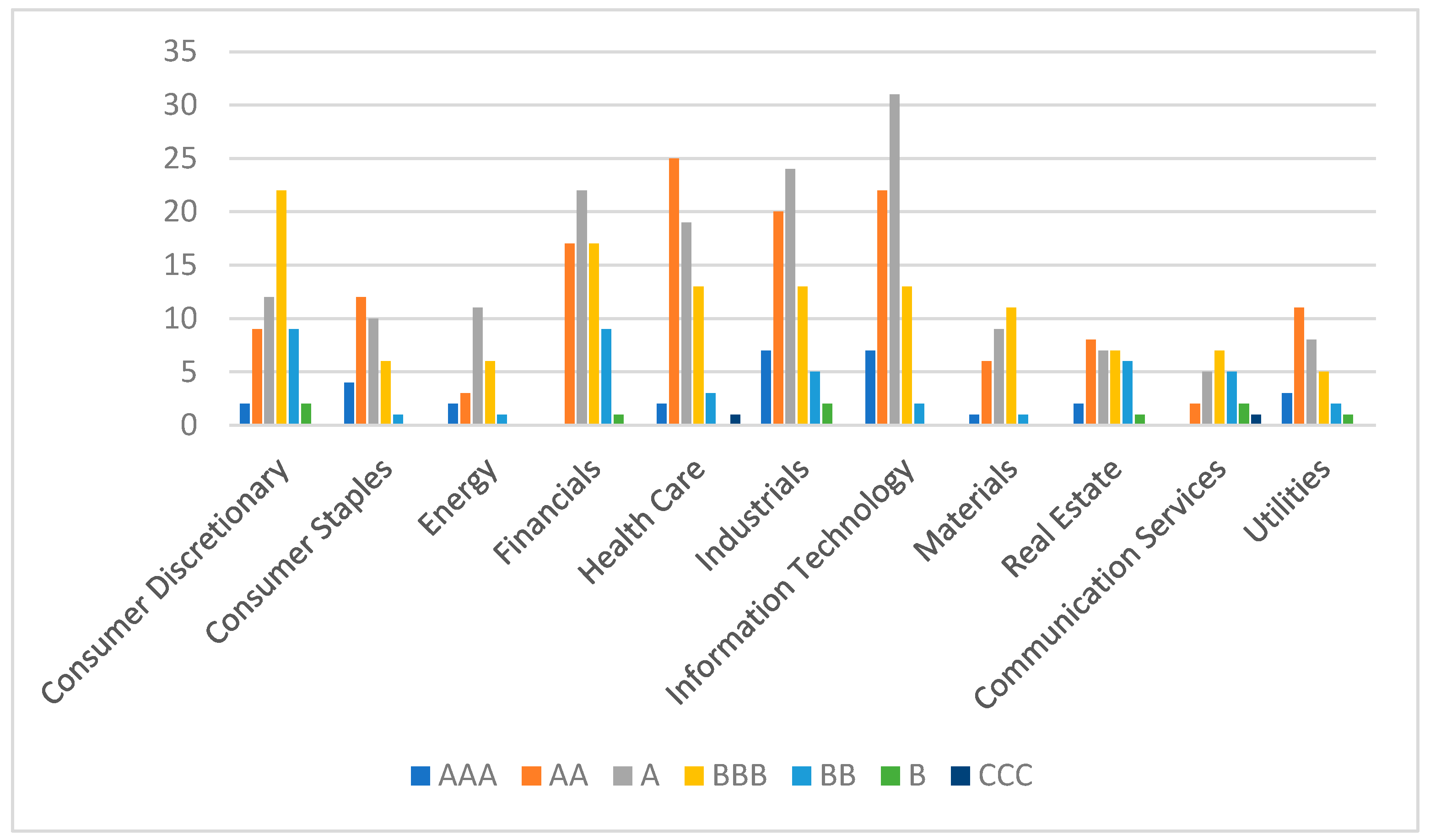
Figure 1 provides an overview of the distribution of companies sampled, showing the number of ESG ratings assigned to each of the AAA, AA, A, BBB, BB, B, and CCC categories for the eleven sectors of the S&P 500 included in our analysis.
3.2. Methods
We analyzed the data in three steps. First, we classified the data into MSCI’s designated categories of Leader (AAA-AA), Average (A-BB), and Laggard (B-CCC). We then calculated key descriptive statistics, including the position parameters minimum, first quartile, median, third quartile, maximum, mean, and standard deviation within the individual categories. Since the comparability of the absolute standard deviation is not possible with different mean values, we used the coefficient of variation, which represents the relative deviation from the mean value and is calculated by dividing the standard deviation by the corresponding mean value. We calculated skewness and excess to further analyze the distribution of the data. By comparing the ratios of descriptive statistics, we may be able to find initial differences within the categories (Leader, Average, and Laggard). For the further steps in our analysis, we made no classification into the MSCI categories, since such classification is only useful for the ratios of the descriptive statistics.
In the second step of our analysis, we used Pearson’s correlation coefficient (Rxy) to test linear relationships between the ESG score and the cost of equity, between the ESG score and the cost of debt, and between the ESG score and the WACC. The formula is
= covariance (); = standard deviation (); = standard deviation ().
= number of observations; = arithmetic mean (); = arithmetic mean ().
Cohen (1988, pp. 79–80) offers this rule of thumb for interpreting the correlation coefficient.
|R| = 0.1 → small effect
|R| = 0.3 → medium effect
|R| = 0.5 → great effect
If at least a small effect of the linear correlation could be determined by the correlation coefficient, we performed a linear regression analysis. For this, however, further conditions must be fulfilled to obtain meaningful results. Jarque and Bera (1980, p. 255) point out that the performance of a regression analysis requires time series independence, a normal distribution, and homoscedasticity of the residuals.
Since the data used here were reference-date-related and were not considered over a longer period, the requirement of time-series independence was fulfilled. To verify the normal distribution assumption, the residuals can be graphically rendered in a “quantile-quantile diagram”, enabling a comparison between the quantiles of the data and the quantiles of the normal distribution (Marden 2004, p. 606). Computationally, the normal distribution of the residuals can be demonstrated by the Jarque–Bera test. Here, the kurtosis of the underlying residuals and the skewness were considered to check whether a normal distribution existed.
S = skewness; = kurtosis; = number of observations.
Subsequently, the value of the Jarque–Bera test statistic was inserted into a chi-square distribution with two degrees of freedom, thereby generating a p-value. In this context, the following pair of hypotheses were made:
Null (H0).
The residuals are normally distributed.
Alternative hypothesis (H1).
The residuals are not normally distributed.
If the p-value is above the significance level of α = 0.05, the null hypothesis cannot be rejected and we can treat the residuals as normally distributed. On the other hand, if the null hypothesis is rejected, there is sufficient evidence that the residuals are not normally distributed.
The third requirement for a valid linear regression analysis is the homoscedasticity of the residuals. They can be evaluated by the eponymous Breusch–Pagan test (Breusch and Pagan 1979). This test is available in Microsoft Excel’s Data Analysis® Add-In Regression Analysis Tool. First, a regression was performed to obtain the residuals. Then, the residuals were squared to perform an auxiliary regression with them. Here, the squared residuals were used as dependent variables and the ESG score as independent variables. The correlation between the squared residuals and the independent variables was then tested by the auxiliary regression. The coefficient of determination calculated by the auxiliary regression was multiplied by the number of observations. This generated the chi-square test statistic. The test statistic was then subjected to a one-degree-of-freedom chi-square distribution test. This resulted in a p-value, which can then be used to make a statement about the presence of homoscedasticity or heteroscedasticity of the residuals. The following hypotheses were made:
Null hypothesis (H0).
The residuals are homoscedastic.
Alternative hypothesis (H1).
The residuals are heteroscedastic.
We again used a significance level of α = 0.05. If the null hypothesis cannot be rejected, there is statistical evidence that we can treat the residuals as homoscedastic. However, if the null hypothesis must be rejected at p < 0.05, then we cannot treat the residuals as homoscedastic.
If time series independence, the normal distribution, and homoscedasticity of the residuals all prevail, we can perform a linear regression analysis. However, if one of the prerequisites is violated, a transformation of the data can be used to attempt to satisfy the prerequisites. Bland and Altman (1996) point out that data are often transformed to analyze them rather than simply evaluating the raw data available. This is because statistical analysis often assumes a certain distribution of the data.
Manikandan (2010) explains that the logarithm, square root, cube root, reciprocal, and square transforms are the most common. Here, he uses some examples to illustrate when each transformation is useful. For example, if the data have a positive skewness, a normal distribution can be achieved using the logarithmic transformation. On the other hand, a square root transformation is useful if the mean and variance are proportional to each other. If the data vary to a large extent and the mean is squared and balanced to the variance, a reciprocal transformation can be applied.
For transforming the data, the root, logarithm, and reciprocal transformation were used for the x and y variable individually as well as together. If it is possible to fulfill the requirements by transforming a single variable, then this combination can be selected. The background is that the transformation should be kept as weak as possible. Table 1 lists the abbreviations of the respective transformations.
If, after applying the transformation to the data, the prerequisites for a regression analysis are still not met, no further analysis is possible. If the prerequisites are fulfilled, we can carry out a linear regression analysis, on the basis of which further evaluation can take place. The first step is to consider the coefficient of determination.
The coefficient of determination gives information about the proportion of the explained variance to the total variance (Nagelkerke 1991, p. 691), taking values between 0 and 1, with a higher value signifying a more complete prediction. The coefficient of determination can be calculated by Equation (4):
= coefficient of determination; = arithmetic mean (); = estimation ().
Finally, we examined the quality of the model using the F-test. If the p-value is lower than the significance level α = 0.05, then the model has a significant explanatory contribution. After transforming the data to perform the linear regression analysis, an inverse transformation was then performed to present the estimated values in an understandable scaling.
4. Results
4.1. Impact of the ESG Rating on the Cost of Equity
We used the capital asset pricing model (CAPM), developed by Sharpe (1964) and Lintner (1965), to calculate the cost of equity:
= cost of equity; = risk free rate; rm = market return; = market risk premium.
Since the risk-free rate and market risk premium apply equally to all companies in the S&P 500, a firm’s beta factor sets its cost of equity. The beta factor can be used to regress it on the ESG score.
Table 2 presents the descriptive statistics of the betas in the Leader, Average, and Laggard categories. It is striking that the median betas (Md) differ by only 0.01 going from Leader to Average, while the mean betas (MV) increase more strongly with lesser ratings, rising from 0.92 (Leader) to 0.98 (Average) to 1.22 (Laggard). The minimum beta (Min) is lowest for Leaders at 0.44 and increases to 0.82 for Laggards, an increase of about 87%. The quartiles and the median (Q1, Md, and Q3) also show an increase in beta as the rating category decreases. The maximum beta (Max) is highest for Leaders at 1.82, and for Laggards, the minimum beta is 1.70.
Overall, we can conclude from the position parameters minimum, first quartile, median, and third quartile that companies with higher ESG ratings have lower betas, which results in a lower cost of equity.
The coefficient of variation (CV) illustrates that the variation in the beta coefficient in each of the three categories is almost identical. Moreover, the skewness (Skew) and excess of Leader and Average hardly deviate from the normal distribution. The excess of Laggard, on the other hand, with −1.28, points to a slightly platykurtic distribution, which minimally reduces the extent of the margins.
The next step is to test for linearity between the ESG rating and beta, for which we use the Pearson correlation coefficient matrix presented in Table 3. This shows that there is a negative linear correlation with a small effect of −0.15 between the ESG rating and the firm’s beta. This suggests a company with a good ESG rating also has a lower beta.
Given the indicated linearity, we check whether we can attempt to regress the beta value as the dependent variable onto the ESG score as the independent variable. Table 4 shows the checks of normal distribution obtained through the Jarque–Bera test. Here, we see that the p-value (ESG/Beta) is less than the significance level of α = 0.05. It follows that the residuals are not normally distributed, and the data must be transformed.
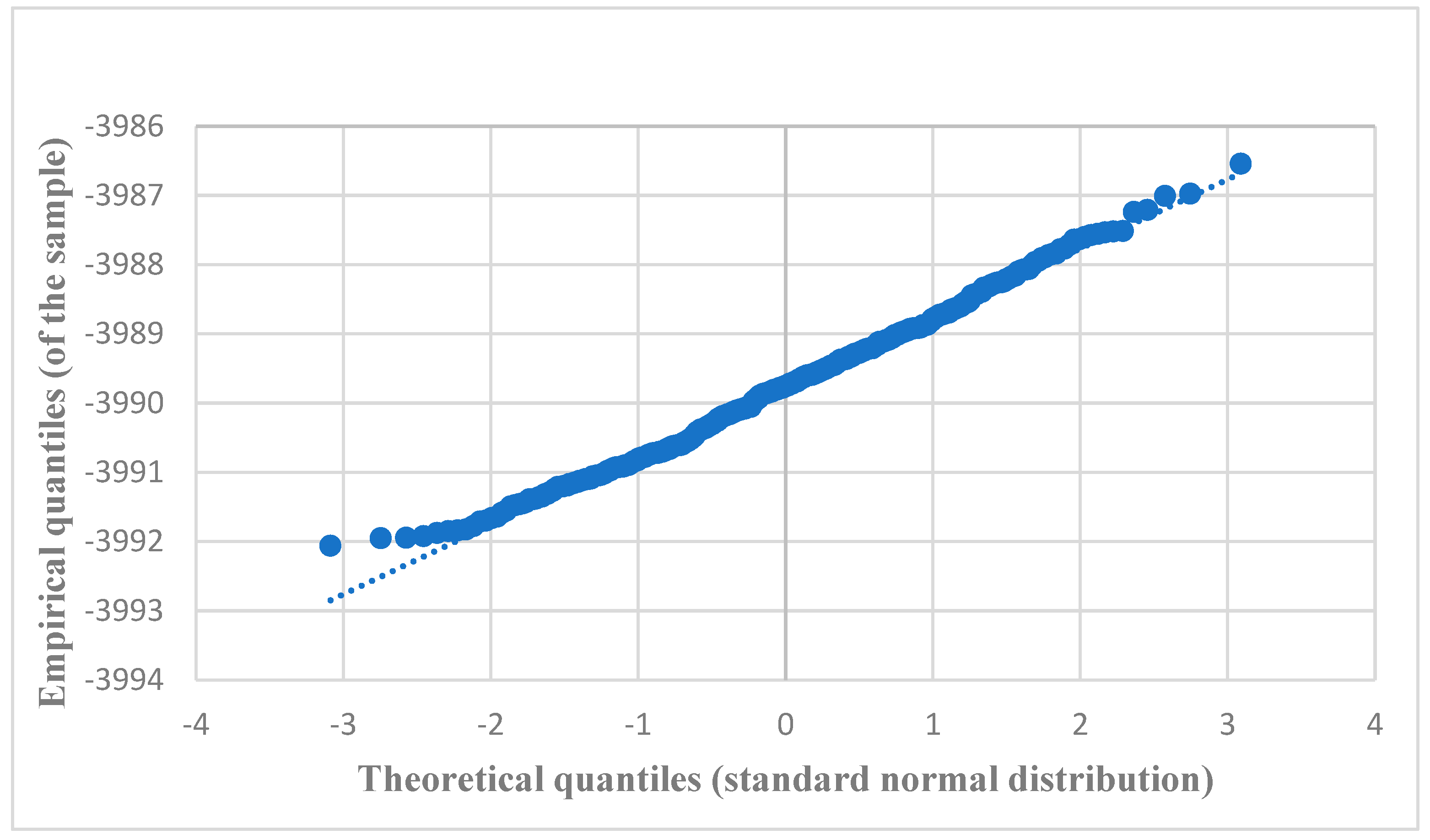
A root transformation of the beta coefficient (y variable) can help in this case. This is shown by the p-value of the Jarque–Bera test. The Jarque–Bera test on the root transformation of beta yields a p-value of 0.13. Thus, the null hypothesis cannot be rejected, and there is no statistical evidence to say that the residuals are anything but normally distributed. In addition, a check using a Q-Q plot of the standardized residuals, shown in Figure 2, makes it clear that the residuals are predominantly located on the straight line, which graphically confirms the normal distribution of the residuals.
The condition of homoscedasticity of the residuals is tested using the Breusch–Pagan test, which shows a p-value of 0.30 as a result. Since the p-value of 0.30 is greater than the significance level of α = 0.05, there is insufficient evidence for an absence of homoscedasticity. Hence, with all preconditions having been met, a linear regression analysis can be performed using the root beta (y variable) and the ESG score (x variable).
Table 5 shows the regression statistics. The evaluation of the linear regression analysis yielded a coefficient of determination of 0.0226. This means that only 2.26% of the variance of the dependent variable (root beta) can be explained by the independent variable (ESG score). In the context of the analysis, the result of the F-test must also be considered, as it provides information about the goodness of the model. The results of the analysis of variance (ANOVA) are presented in Table 6. The regression model shows a p-value of 0.001, which is significantly lower than the significance level of α = 0.05. This means that the regression model is significant for the independent variable (ESG score). This indicates that the regression model makes a statistically significant explanatory contribution.
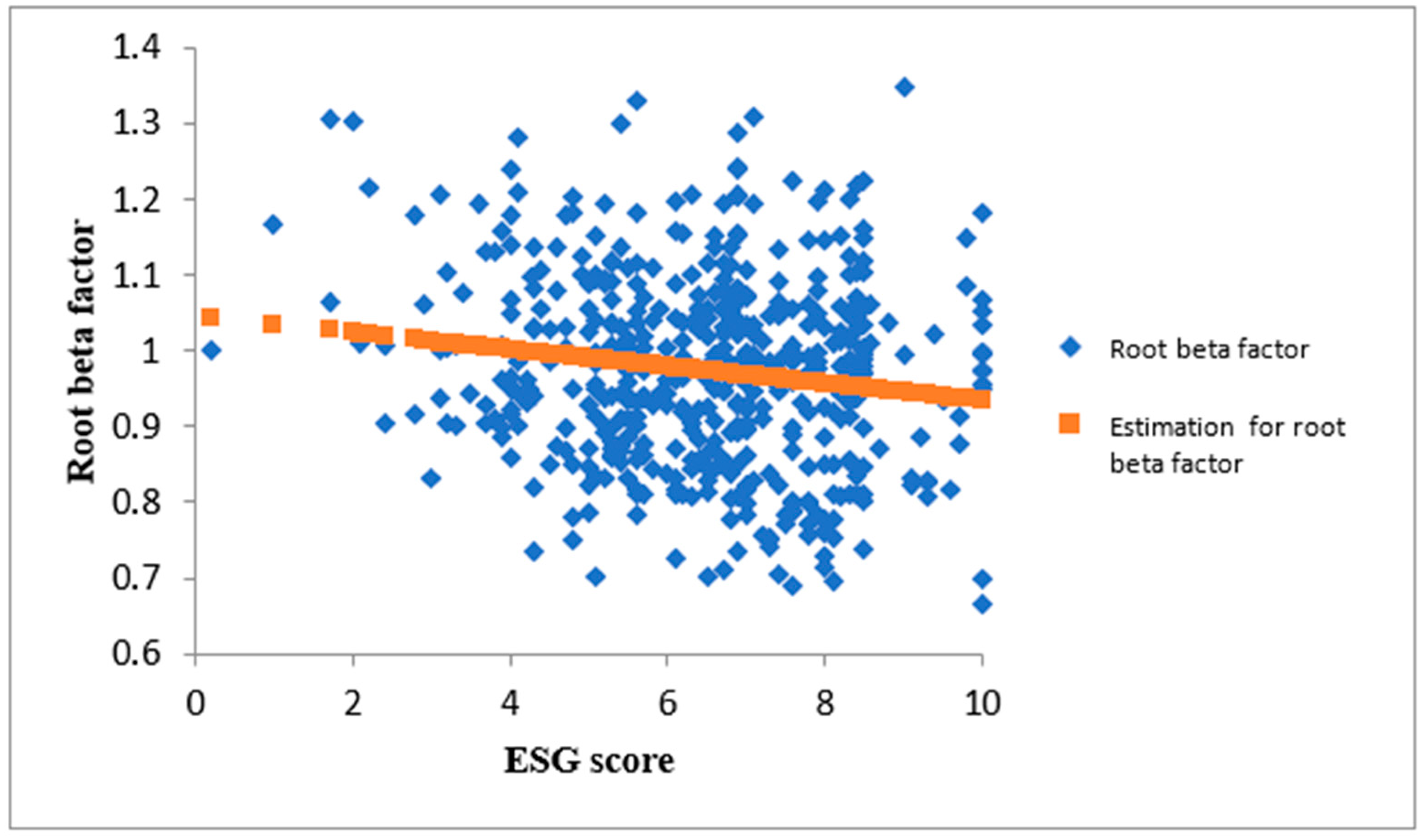
Next, we consider the estimated constant, computed as 1.046. It follows that an ESG score of zero yields by the model an estimated root beta of 1.046. The slope parameter is equal to −0.0112, which means that a one unit increase in the ESG score leads to a 0.0112 unit decrease in the root beta. The estimate for the root beta is shown on the scatterplot of Figure 3. The estimated visualization can be improved by more comprehensible scaling using an inverse transformation of the estimates. Currently, the estimate takes the following form:
Subsequently, the data are transformed by squaring both sides of the equation. Thus, the radical sign of the estimate of the root beta is resolved and the following equation results:
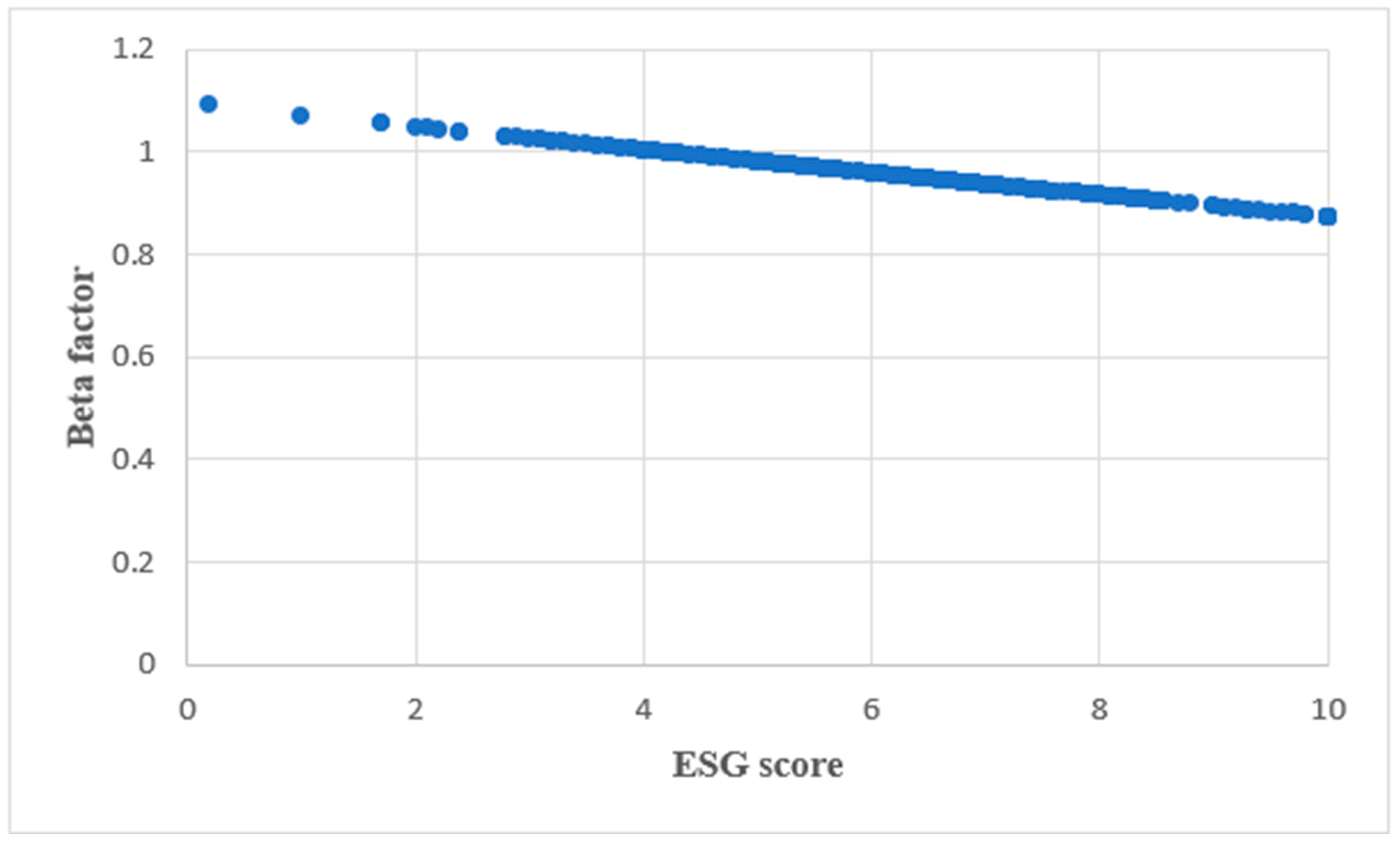
By back-transformation, the estimates of the beta can now be illustrated with the corresponding ESG score in Figure 4. This shows that an increase in ESG score of 10 leads to a decrease in beta from 1.1 to about 0.85, or a 0.25 decrease.
The results of the descriptive statistics suggest that companies with a lower ESG rating have a higher beta factor.
4.2. Impact of the ESG Rating on the Cost of Debt
The cost of debt per rating category is summarized by the descriptive statistics in Table 7. The first quartile, the median, and the third quartile each show an increase in the cost of debt from Leader to Laggard. In the first quartile, the cost of debt increases by approximately 7.7%, from 3.9% (Leader) to 4.2% (Laggard). Within the third quartile, an increase of about 15.5%, namely from 4.5% (Leader) to 5.2% (Laggard), can be observed. A similar result is provided by the mean value, which is significantly lower for the Leaders (4.3%) than for Laggard (4.8%). This indicates that companies with a poor ESG rating must bear a significantly higher cost of debt than companies with a good ESG rating. Similar results are obtained when comparing the Average and Laggard categories. The minimum, first quartile, median, third quartile, and mean ratios are lower in the Average category than in the Laggard, showing again that companies with a poor ESG rating face a higher cost of debt.
The coefficient of variation is nearly identical in all categories. The excess, on the other hand, shows that in the Leader (3.16) and Average (3.8) categories, the marginal ranges of the distribution of the cost of debt are significantly more pronounced than in the Laggard category. Within the Laggard category, the distribution of cost of debt is slightly skewed to the right.
For further analysis, the linearity between the ESG score and the cost of debt can be estimated by the Pearson correlation coefficient; the result of the calculation, −0.17, indicates a negative linear relationship with a small effect. This is consistent with the claim that companies with a higher ESG score have a lower cost of debt.
We next examine whether it is possible to perform a linear regression analysis. The results of the Jarque–Bera test are listed in Table 8. Here, no normal distribution of the residuals could be found, as the p-value is 0.00. Even transforming the data could not cure the violation of the normal distribution assumption. All transformations performed resulted in an unchanged p-value of 0.00.
Since the condition of normal distribution was violated in all cases, a further test of the homoscedasticity of the residuals using the Breusch–Pagan test would not have been meaningful. As a result, we are not permitted to regress the cost of debt onto the ESG score.
The ratios of descriptive statistics in Table 7, however, show that companies with a good-to-medium ESG rating benefit from a lower cost of debt. Furthermore, the correlation effect confirms a negative linear relationship with a small effect between ESG score and cost of debt. Further analysis using a regression analysis cannot be performed.
4.3. Impact of the ESG Rating on the WACC
Table 9 presents the descriptive statistics for the WACC across the three ESG rating categories. The maximum for Leader is 11.9%, while for Laggard, it is only 9.1%. It is striking that Laggard has the lowest WACC for the first quartile (6.2%) and the third quartile (7.8%). Additionally, the minimum of 4.9% is found by Averages. Furthermore, Laggards have a significantly lower mean value of 7.0% than Average (7.6%) and Leader (7.5%). A similar result can be found with the median. The median for Average and Leader is 7.4%, which is 70 basis points higher than for Laggard. These results point to companies with a lower ESG rating having a lower WACC than companies with a higher ESG rating.
Furthermore, the slight increase in the coefficient of variation from Laggard (0.15) to Average (0.17) to Leader (0.17) is striking. Thus, the relative standard deviation of the WACC is slightly increased within the categories comprising firms with a good rating. The skewness is positive in all three categories. Thus, the data distribution is right-skewed, meaning more firms have a lower WACC than would be expected for a normal distribution. The positive excess in the Leader and Average categories indicates that more extreme values occur within these categories than in the Laggard category.
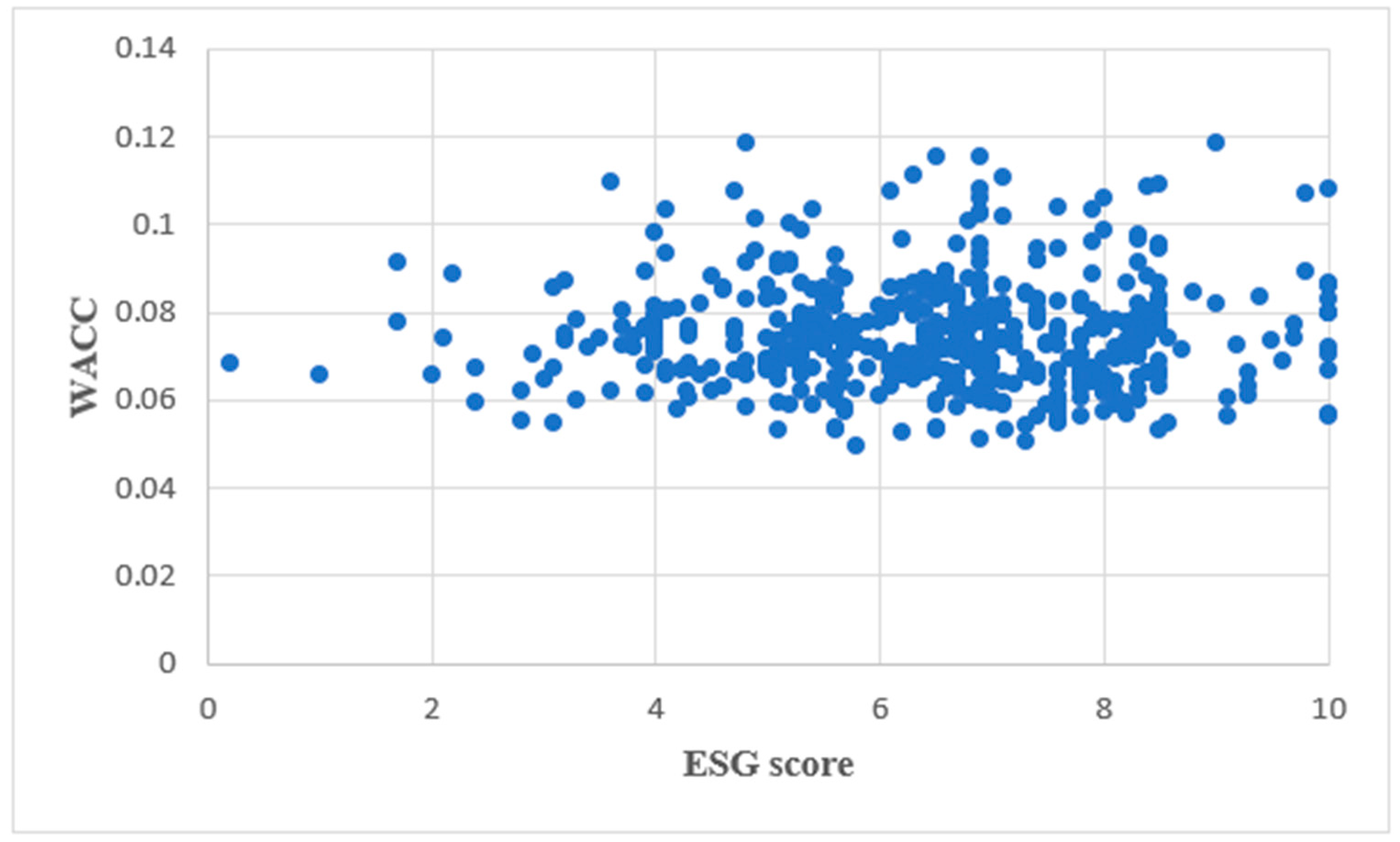
Our first step of evaluating the descriptive statistics reveals that a good ESG rating does not lead to a lower WACC. We confirm this by checking for a linear relationship between the WACC and the ESG score using the correlation coefficient; with a value of 0.04, the coefficient indicates no effect. Figure 5 plots a featureless cloud of points for the WACC and the ESG rating. Transforming the data makes no sense, as there is already a very low correlation coefficient that would only improve minimally. It follows that performing a linear regression analysis would not make sense.
Since the WACC considers the proportion of debt and equity in the total capital in the calculation, the difference in the WACC may be due to the different capital structure of the companies. The formula of the WACC is
= cost of debt; = tax rate; = equity; = debt.
In the first step, we examine whether there is a linear relationship between the ESG score and the debt ratio. At −0.18, the correlation coefficient between the ESG score and the debt ratio indicates a negative linear relationship with a small effect. This leads us to suggest that a lower WACC reflects the combination of a lower cost of debt coupled to a higher leverage ratio.
For verification, an analysis of the debt ratio is performed using the descriptive statistics ratios, with the results listed in Table 10. It is striking that the first quartile for Laggard, at 17.6%, is approximately 74.5% higher than for the Leader category, at 10.2%. Similar results are observed in the third quartile, the mean, and the median. Moreover, the mean value of 47.8% for Laggard is more than twice the mean value for Leader, which is 22.5%. The maximum of the debt ratio is 85.1% for Laggard, significantly higher than Leader’s maximum of 70.3%.
The analysis of the descriptive statistics indicates that companies with a poor ESG rating have a higher debt ratio. If a company is characterized by a higher debt ratio, the equity ratio is correspondingly lower. We thus calculate the mean value of the cost of equity and compare that to the mean value of the cost of debt within the individual categories. The mean value of the cost of equity increases further from Leader (8.3%) to Average (8.6%) and to Laggard (9.1%). Furthermore, by comparing Table 10 and Table 11, it can be seen that in all three categories, the cost of equity is significantly higher than the cost of debt. The difference is 0.8% for the Leader category, 1.0% for Average, and 2.1% for Laggard. We thus conclude that indeed the lower WACC for companies with a poorer ESG rating is due to the combination of the lower cost of debt and a significantly higher leverage ratio. Companies with a good ESG rating have a higher equity ratio, which, together with a higher cost of equity, results in a higher WACC.
The results of the descriptive statistics show that a better ESG rating does not lead to a reduction in the WACC. Furthermore, there is no linear correlation between the WACC and the ESG score, as the latter has no effect on the former. We conclude that companies with a poor ESG rating have a lower WACC due to the higher proportion of debt capital, coupled with the higher cost of debt, compared to the cost of equity capital.
5. Discussion
Our analysis aimed to investigate the impact of ESG ratings on the cost of capital for companies in the U.S. market, specifically those constituting the S&P 500. We focused our equity analysis on the firm’s beta, the risk premium coefficient in the capital asset pricing model (CAPM), which we use to calculate the cost of equity. Analysis of the descriptive statistics of the beta distribution shows that firms with a better ESG rating benefit from a lower beta. This provides an answer to research question one: based on the descriptive statistics, favorable ESG ratings lower the cost of equity for companies in the S&P 500.
We also observe a slightly negative linear relationship between the ESG score and beta, and a negative correlation between the ESG score and the root transformation of beta was confirmed by linear regression analysis. The regression model has statistical significance. Back-transforming the beta estimate then shows lower betas with higher ESG scores. Continuing our use of the CAPM to calculate the cost of equity, research question two can be answered: an increase in the ESG score lowers the cost of equity. Similar results were provided by the research of Gonçalves et al. (2022) and Chen et al. (2023).
Research question three—“What do descriptive statistics say about the impact of ESG rating on the cost of debt for companies in the S&P 500?”—can be answered as follows: descriptive statistics show that a poor ESG rating leads to an increase in the cost of debt. Moreover, to answer our fourth research question, we can report that a negative linear relationship with a small effect (−0.17) can be found between ESG score and cost of debt. This is consistent with the results of Arora and Sharma (2022).
In contrast, analysis by descriptive statistics could find no improvement in the WACC with higher ESG ratings. Instead, the statistics show that the companies with better ESG ratings have minimally increased WACCs. As a result, no effect of ESG rating on WACC could be proven with respect to research question five. Furthermore, no effect could be found in terms of a linear relationship between the WACC and the ESG score. Thus, research question six can be answered: there is no linear relationship between the ESG score and the WACC. Using the correlation coefficient as the criterion, we find no effect of the ESG score on the WACC.
We conducted a capital structure analysis to gain further insight into this result. The analysis demonstrates that firms with a lower ESG rating have a higher debt ratio. Since the cost of debt is lower compared to the cost of equity, this leads to a lower WACC for these firms. Assuming central banks leave the key interest rate at an elevated level, companies with a low ESG rating will eventually have to feel this fact when refinancing in the future. As a result, companies with a poor ESG rating are likely to report a significantly higher WACC in the future. If lenders were to factor ESG rating more strongly into their future terms, this effect would be amplified.
Further research is needed into the impact of ESG rating on the cost of capital. First, it makes sense to analyze other indices, such as the Dax 40 or the FTSE 100, to corroborate the importance of ESG for developed capital markets. Furthermore, the ESG rating should be broken down into individual components (environment, social, and governance) to be able to make precise statements about the relevance of individual ESG factors to the capital markets. Using data over a longer period of time for the analysis would also be interesting, although securing adequate high-quality data could be a challenge. Other possibilities include conducting an analysis based on various regression models.
It would also make sense to add a control variable to the regression model in order to take possible confounding factors into account. This would isolate the relationship between ESG rating and cost of capital and ensure that the observed relationship is not influenced by other unobserved factors.
We predict that in the future, a firm’s sustainability criteria will be priced into its refinancing costs. This is the market encouraging sustainable corporate management by rewarding sustainably managed firms with lower capital costs.
Author Contributions
Conceptualization, D.E. and F.W.; methodology, D.E. and F.W.; software, F.W.; validation, D.E. and F.W.; formal analysis, D.E. and F.W.; investigation, D.E. and F.W.; resources, D.E. and F.W.; data curation, F.W.; writing—original draft preparation, D.E. and F.W.; writing—review and editing, D.E. and F.W.; visualization, F.W.; supervision, D.E. and F.W.; project administration, D.E. and F.W.; funding acquisition, D.E. All authors have read and agreed to the published version of the manuscript.
Funding
This research received no external funding.
Institutional Review Board Statement
Not applicable.
Informed Consent Statement
Not applicable.
Data Availability Statement
Data are contained within the article.
Conflicts of Interest
The authors declare no conflicts of interest.
References
- Arora, Ankit, and Dipasha Sharma. 2022. Do Environmental, Social and Governance (ESG) Performance Scores Reduce the Cost of Debt? Evidence from Indian firms. Australasian Business, Accounting and Finance Journal 16: 4–18. [Google Scholar] [CrossRef]
- Atan, Ruhaya, Md. Mahmudul Alam, Jamaliah Said, and Mohamed Zamri. 2018. The impacts of environmental, social, and governance factors on firm performance. Management of Environmental Quality 29: 182–94. [Google Scholar] [CrossRef]
- Bellavite Pellegrini, Carlo, Raul Caruso, and Niketa Mehmeti. 2019. The impact of ESG scores on cost of equity and firm’s profitability. New Challenges in Corporate Governance: Theory and Practice, 38–40. [Google Scholar]
- Bland, J. Martin, and Douglas G. Altman. 1996. Transforming data. BMJ 312: 770. [Google Scholar] [CrossRef] [PubMed]
- Bloomberg Intelligence. 2021. ESG Assets May Hit $53 Trillion by 2025, a Third of Global AUM. Available online: https://www.bloomberg.com/professional/blog/esg-assets-may-hit-53-trillion-by-2025-a-third-of-global-aum/ (accessed on 10 February 2023).
- Breusch, Trevor S., and Adrian R. Pagan. 1979. A Simple Test for Heteroscedasticity and Random Coefficient Variation. Econometrica 47: 1287–94. [Google Scholar] [CrossRef]
- Chen, Mike, Robert von Behren, and George Mussalli. 2021. The Unreasonable Attractiveness of More ESG Data. The Journal of Portfolio Management 48: 147–62. [Google Scholar] [CrossRef]
- Chen, Yonghuai, Tao Li, Qing Zeng, and Bo Zhu. 2023. Effect of ESG performance on the cost of equity capital: Evidence from China. International Review of Economics & Finance 83: 348–64. [Google Scholar] [CrossRef]
- Chouaibi, Yamina, Matteo Rossi, and Ghazi Zouari. 2021. The Effect of Corporate SocialResponsibility and the Executive Compensation on Implicit Cost of Equity: Evidence from French ESG Data. Sustainability 13: 1510. [Google Scholar] [CrossRef]
- Cohen, Jacob. 1988. Statistical Power Analysis for the Behavioral Sciences, 2nd ed. New York: Routledge. [Google Scholar]
- Dahiya, Monika, and Shveta Singh. 2021. The linkage between CSR and cost of equity: An Indian perspective. Sustainability Accounting, Management and Policy Journal 12: 499–521. [Google Scholar] [CrossRef]
- Dahlsrud, Alexander. 2008. How corporate social responsibility is defined: An analysis of 37 definitions. Corporate Social Responsibility and Environmental Management 15: 1–13. [Google Scholar] [CrossRef]
- Daugaard, Dan, and Ashley Ding. 2022. Global Drivers for ESG Performance: The Body of Knowledge. Sustainability 14: 2322. [Google Scholar] [CrossRef]
- Dhaliwal, Dan S., Oliver Zhen Li, Albert Tsang, and Yong George Yang. 2011. Voluntary Nonfinancial Disclosure and the Cost of Equity Capital: The Initiation of Corporate Social Responsibility Reporting. The Accounting Review 86: 59–100. [Google Scholar] [CrossRef]
- Europäische Kommission. 2001. Europäische Rahmenbedingungen für die sozialeVerantwortung der Unternehmen. Available online: https://eur-lex.europa.eu/LexUriServ/LexUriServ.do?uri=COM:2001:0366:FIN:de:PDF (accessed on 10 February 2023).
- Gigante, Gimede, and Davide Manglaviti. 2022. The ESG effect on the cost of debt financing: A sharp RD analysis. International Review of Financial Analysis 84: 102382. [Google Scholar] [CrossRef]
- Gonçalves, Tiago Cruz, João Dias, and Victor Barros. 2022. Sustainability Performance and the Cost of Capital. International Journal of Financial Studies 10: 63. [Google Scholar] [CrossRef]
- Goss, Allen, and Gordon S. Roberts. 2011. The impact of corporate social responsibility on the cost of bank loans. Journal of Banking & Finance 35: 1794–810. [Google Scholar] [CrossRef]
- Jarque, Carlos M., and Anil K. Bera. 1980. Efficient tests for normality, homoscedasticity and serial independence of regression residuals. Economics Letters 6: 255–59. [Google Scholar] [CrossRef]
- Johnson, Ruth. 2020. The link between environmental, social and corporate governance disclosure and the cost of capital in South Africa. Journal of Economic and Financial Sciences 13: 1–12. [Google Scholar] [CrossRef]
- Khanchel, Imen, and Naima Lassoued. 2022. ESG Disclosure and the Cost of Capital: Is There a Ratcheting Effect over Time? Sustainability 14: 9237. [Google Scholar] [CrossRef]
- Lin-Hi, Nick, and Karsten Müller. 2013. The CSR Bottom Line: Preventing Corporate Social Irresponsibility. Journal of Business Research 66: 1928–36. [Google Scholar] [CrossRef]
- Lintner, John. 1965. The Valuation of Risk Assets and the Selection of Risky Investments in Stock Portfolios and Capital Budgets. The Review of Economics and Statistics 47: 13–37. [Google Scholar] [CrossRef]
- Manikandan, S. 2010. Data transformation. Journal of Pharmacology & Pharmacotherapeutics 1: 126–27. [Google Scholar] [CrossRef]
- Marden, John I. 2004. Positions and QQ Plots. Statistical Science 19: 606–14. [Google Scholar] [CrossRef]
- Nagelkerke, Nico J. D. 1991. A Note on a General Definition of the Coefficient of Determination. Biometrika 78: 691–92. [Google Scholar] [CrossRef]
- PricewaterhouseCoopers International. 2022. ESG-Focused Institutional Investment Seensoaring 84% to US$33.9 Trillion in 2026, Making up 21.5% of Assets under Management: PwC Report. Available online: https://www.pwc.com/gx/en/news-room/press-releases/2022/awm-revolution-2022-report.html (accessed on 10 December 2022).
- Raimo, Nicola, Alessandra Caragnano, Marianna Zito, Filippo Vitolla, and Massimo Mariani. 2021. Extending the benefits of ESG disclosure: The effect on the cost of debt financing. Corporate Social Responsibility and Environmental Management 28: 1412–21. [Google Scholar] [CrossRef]
- Richardson, Alan J., and Michael Welker. 2001. Social disclosure, financial disclosure and the cost of equity capital. Accounting, Organizations and Society 26: 597–616. [Google Scholar] [CrossRef]
- Sharpe, William F. 1964. Capital Asset Prices: A Theory of Market Equilibrium under Conditions of Risk. The Journal of Finance 19: 425–42. [Google Scholar] [CrossRef]
- United Nations. 2004. Who Cares Wins. Available online: https://www.unepfi.org/fileadmin/events/2004/stocks/who_cares_wins_global_compact_2004.pdf (accessed on 10 February 2023).
- Wong, Woei Chyuan, Jonathan A. Batten, Abd Halim Ahmad, Shamsul Bahrain Mohamed-Arshad, Sabariah Nordin, and Azira Abdul Adzis. 2021. Does ESG certification add firm value? Finance Research Letters 39: 101593. [Google Scholar] [CrossRef]
Figure 1.
ESG rating of the analyzed companies per sector (S&P 500).

Figure 2.
Q-Q plot of residuals (ESG score/root beta factor).

Figure 3.
Estimation of the root beta factor.

Figure 4.
Estimation of the beta factor.

Figure 5.
Point cloud of WACC/ESG score.


Table 1.
Abbreviations of the data transformations.
| “Root” | “LN” | “1/” |
|---|---|---|
| Root transformation | Logarithm transformation | Reciprocal transformation |
Table 2.
Descriptive statistics of the beta factor.
| Min | Q1 | Md | Q3 | Max | MV | STDV | CV | Excess | Skew | |
| Leader | 0.44 | 0.69 | 0.94 | 1.07 | 1.82 | 0.92 | 0.25 | 0.28 | 0.12 | 0.42 |
| Average | 0.49 | 0.80 | 0.95 | 1.11 | 1.77 | 0.98 | 0.24 | 0.25 | 0.46 | 0.62 |
| Laggard | 0.82 | 1.00 | 1.13 | 1.48 | 1.70 | 1.22 | 0.31 | 0.25 | −1.28 | 0.33 |
Table 3.
Pearson correlation matrix.
| ESG-Rating | Beta | re | e-Ratio | rd | d-Ratio | WACC | |
| ESG-Rating | 1.00 | ||||||
| Beta | −0.15 | 1.00 | |||||
| re | −0.11 | 0.92 | 1.00 | ||||
| e-ratio | 0.18 | 0.02 | 0.05 | 1.00 | |||
| rd | −0.17 | 0.11 | 0.09 | −0.28 | 1.00 | ||
| d-ratio | −0.18 | −0.03 | −0.05 | −1.00 | 0.28 | 1.00 | |
| WACC | 0.04 | 0.68 | 0.76 | 0.64 | 0.05 | −0.64 | 1.00 |
Table 4.
Jarque–Bera test for beta factor (p-value).
| ESG | LN ESG | W ESG | 1/ESG | |
| Beta | 0.00 | 0.00 | 0.00 | 0.00 |
| LN Beta | 0.18 | 0.16 | 0.18 | 0.17 |
| Root Beta | 0.13 | 0.14 | 0.13 | 0.22 |
| 1/Beta | 0.00 | 0.00 | 0.00 | 0.00 |
Table 5.
Regression statistics (ESG score/root beta factor).
| Coefficient of determination | 0.0226 |
| Adjusted coefficient of determination | 0.0206 |
| Standard error | 0.1251 |
| Observations | 498 |
Table 6.
ANOVA (ESG score/root beta factor).
| Degrees of Freedom | Sum of Squares | Mean Square Sum | Test Variable (F) | F Crit | |
| Regression | 1 | 0.179 | 0.179 | 11.465 | 0.001 |
| Residuals | 496 | 7.759 | 0.016 | ||
| Overall | 497 | 7.938 |
Table 7.
Descriptive statistics of the cost of debt.
| Min | Q1 | Md | Q3 | Max | MV | STDV | CV | Excess | Skew | |
| Leader | 0.019 | 0.039 | 0.042 | 0.045 | 0.062 | 0.043 | 0.007 | 0.153 | 3.156 | −0.107 |
| Average | 0.011 | 0.039 | 0.042 | 0.045 | 0.065 | 0.042 | 0.007 | 0.155 | 3.786 | −0.024 |
| Laggard | 0.036 | 0.042 | 0.049 | 0.052 | 0.065 | 0.048 | 0.008 | 0.164 | 0.617 | 0.693 |
Table 8.
Jarque–Bera test for cost of debt (p-value).
| ESG | LN ESG | W ESG | 1/ESG | |
| rd | 0.00 | 0.00 | 0.00 | 0.00 |
| LN rd | 0.00 | 0.00 | 0.00 | 0.00 |
| W rd | 0.00 | 0.00 | 0.00 | 0.00 |
| 1/rd | 0.00 | 0.00 | 0.00 | 0.00 |
Table 9.
Descriptive statistics of WACC.
| WACC | Min | Q1 | Md | Q3 | Max | MV | STDV | CV | Excess | Skew |
| Leader | 0.051 | 0.065 | 0.074 | 0.082 | 0.119 | 0.075 | 0.013 | 0.174 | 0.518 | 0.736 |
| Average | 0.049 | 0.067 | 0.074 | 0.081 | 0.116 | 0.076 | 0.013 | 0.168 | 1.110 | 0.881 |
| Laggard | 0.055 | 0.062 | 0.067 | 0.078 | 0.091 | 0.070 | 0.011 | 0.154 | −0.201 | 0.764 |
Table 10.
Descriptive statistics of debt ratio.
| Min | Q1 | Md | Q3 | Max | MV | STDV | CV | Excess | Skew | |
| Leader | 0.001 | 0.102 | 0.203 | 0.327 | 0.703 | 0.225 | 0.152 | 0.675 | −0.074 | 0.705 |
| Average | 0.001 | 0.113 | 0.214 | 0.332 | 0.842 | 0.244 | 0.176 | 0.720 | 1.170 | 1.083 |
| Laggard | 0.038 | 0.176 | 0.483 | 0.751 | 0.851 | 0.478 | 0.280 | 0.586 | −1.431 | −0.334 |
Table 11.
Descriptive statistics of cost of equity.
| Min | Q1 | Md | Q3 | Max | MV | STDV | CV | Excess | Skew | |
| Leader | 0.059 | 0.073 | 0.084 | 0.089 | 0.121 | 0.083 | 0.012 | 0.144 | 0.244 | 0.399 |
| Average | 0.058 | 0.077 | 0.086 | 0.092 | 0.125 | 0.086 | 0.011 | 0.131 | 1.021 | 0.624 |
| Laggard | 0.073 | 0.080 | 0.092 | 0.106 | 0.114 | 0.092 | 0.012 | 0.135 | −0.842 | 0.423 |
Disclaimer/Publisher’s Note: The statements, opinions and data contained in all publications are solely those of the individual author(s) and contributor(s) and not of MDPI and/or the editor(s). MDPI and/or the editor(s) disclaim responsibility for any injury to people or property resulting from any ideas, methods, instructions or products referred to in the content. |
© 2024 by the authors. Licensee MDPI, Basel, Switzerland. This article is an open access article distributed under the terms and conditions of the Creative Commons Attribution (CC BY) license (https://creativecommons.org/licenses/by/4.0/).
Share and Cite
MDPI and ACS Style
Ernst, D.; Woithe, F. Impact of the Environmental, Social, and Governance Rating on the Cost of Capital: Evidence from the S&P 500. J. Risk Financial Manag. 2024, 17, 91. https://doi.org/10.3390/jrfm17030091
AMA Style
Ernst D, Woithe F. Impact of the Environmental, Social, and Governance Rating on the Cost of Capital: Evidence from the S&P 500. Journal of Risk and Financial Management. 2024; 17(3):91. https://doi.org/10.3390/jrfm17030091
Chicago/Turabian StyleErnst, Dietmar, and Florian Woithe. 2024. "Impact of the Environmental, Social, and Governance Rating on the Cost of Capital: Evidence from the S&P 500" Journal of Risk and Financial Management 17, no. 3: 91. https://doi.org/10.3390/jrfm17030091