1. Introduction
Understandable algorithms, low-frequency trading, better performance, and avoiding drawdown are investors’ desired goals in the stock market. We applied only two oscillators to measure the trading of index ETFs. Simulation trading results have shown positive measurements corresponding to accepting investments immediately. Regarding individual investors and low-frequency institutional investors, a tool needs to be established for them.
The modern portfolio theory (
Elton et al. 2014;
Markowitz 1952) is orthodox in the investment field. In modern portfolio theory (MPT) investment, the efficient frontier line is an important standard to invest in. At present, MPT investment is the most commonly accepted established investment strategy.
Camanho et al. (
2022) published a paper on portfolio rebalancing that effectively discussed multiple macroeconomic factors. Another study suggested that high-frequency trading could provide liquidity and reduce net costs for long-term investors (
Bershova and Rakhlin 2013). Furthermore,
Liu et al. (
2022) built a high-frequency trading model to maximize returns from the point of view of the risk–return profile. However, the market’s random path neutralizes EMH and MPT (
Ng and Suo 2022;
Sherlock et al. 2010). In response to these trends in the stock market, we conducted research to help with investment in other ways. Many past studies have attempted to achieve this through descriptive, quantitative, and qualitative analyses. We tested how to respond to the market’s random nature through using technical indicators. High-frequency trading studies dominate when looking for trading methodologies, high-frequency trading studies dominate. In the case of high-frequency trading, specialized skills, technical support for trading, high-speed communication, and increased transaction costs due to many trades have become limitations for individual investors, pension investors, and small institutional investors.
The previous studies on index forecasting using stochastics for signal, MPT, and high-frequency trading represent a research area that has become popular in recent years. However, few studies on low-frequency trading according to the index direction combined with signal use exist. This paper aims to investigate a simple and general trading model. We focused on estimating overbought and oversold stock market indices and translating them into real-world investments. We tested and presented simulated trades on tracking indices and the ETFs that use them as benchmarks and have the largest AUM. Next, we targeted low-frequency trading for retail investors, pension investors, and small institutional investors who may be unable to use high-frequency trading techniques. With low-frequency trading, we attempted to focus on increasing the realized return and hit ratio and on reducing the maximum drawdown. The findings of this study will be useful for scholars and stakeholders, particularly those seeking positive investment results, low-cost fees, and a new methodology centered around understandable algorithm trading and the easy acceptance of trading.
MPT investment depends on the risk–return profile, which is also changeable depending on the financial environment, so investors must rebalance their portfolios periodically. However, not all investors have access to information resources regarding MPT or adequate knowledge of it, so we used the ETF and weight for simple trading. In the case of the U.S. market, index, and sector, using the moving average market timing model without MPT’s rebalancing has been shown to lead to positive results (
Topiwala 2023b;
Mukerji et al. 2019). Moreover, the buy-and-hold strategy, based on the moving average, has been shown to achieve a better CAPM alpha than the index without rebalancing (
Huang and Huang 2020).
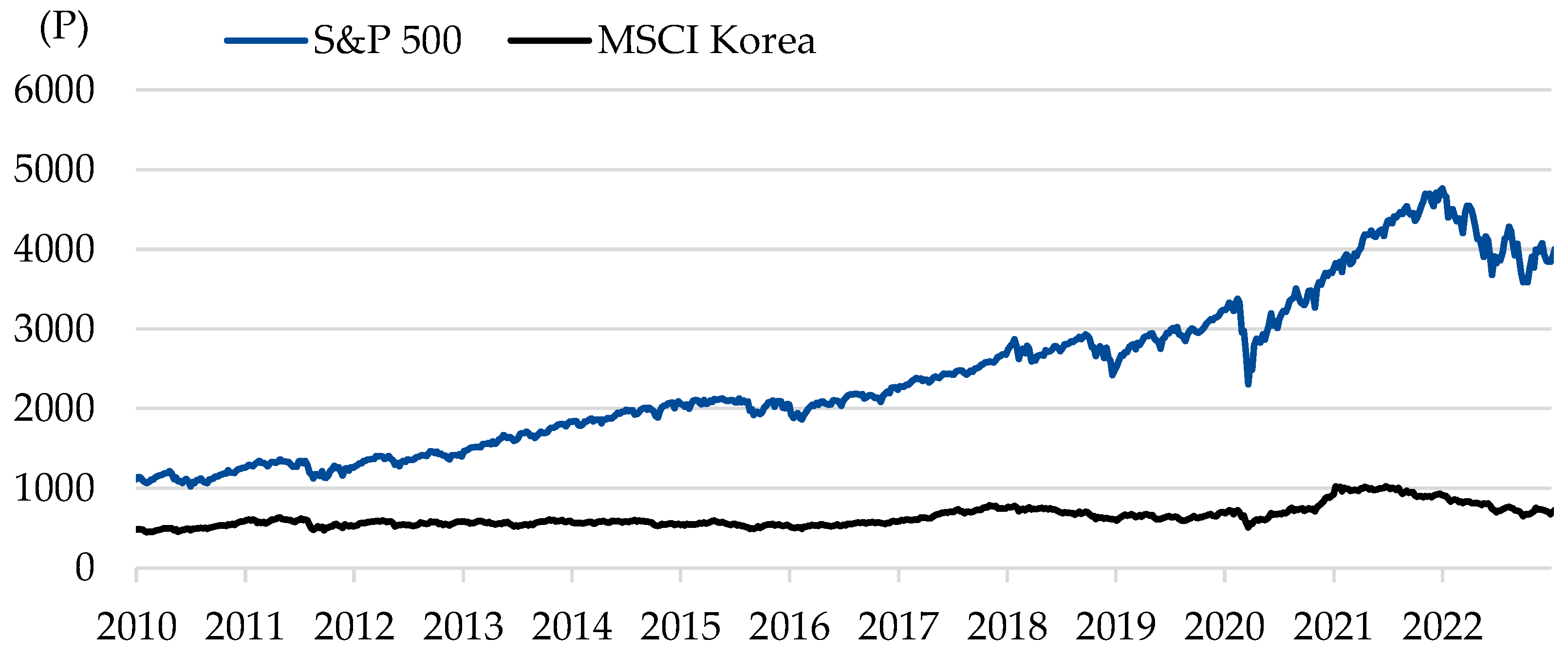
We tested the U.S. and Korean market indices via comparison and combination. The S&P 500 US market index is the significant index in the MSCI ACWI and MSCI WORLD indices, which are representative benchmark indices. Institutional and individual investors compare the return rate to the benchmark. In this situation, the most weighted index is an important index to invest in and simulate. Also, the MSCI KOREA index is the second most significant index in the MSCI EM index, the benchmark in the emerging stock market. After 2018, the U.S. experienced heavy conflict with China, causing a prolonged downtrend in the Chinese stock market. We studied these two critical indices in both developed and emerging markets. The two indices differ with respect to the following: developed economy vs. emerging economy, key currency vs. non-key currency, size of the market, and political power. The U.S. stock market index constantly grew after the 2008 financial crisis, while the EM stock market shows a sideways trend and is more volatile.
We traded two ETFs: first, SPY instead of the S&P 500, which is representative of the U.S. market, and second, EWY instead of MSCI Korea. Herein, we present results for each ETF and combine two ETFs for comparison and analysis. Our study was conducted under trading time limitations to help demonstrate how to achieve low-frequency goals and positive results as a small individual investor. We fixed the weight of ETF in the combined portfolio without adjusting asset allocation.
Our trading algorithm, DeepSignal, consists of two technical trading signals based on moving average periods. The first is a stochastic oscillator, and the second is William%R. We tested multiple periods and levels. Herein, we present the core components of our algorithm-based statistical approach. Moreover, we limited the average number of trades to only one a month. This low-frequency trading and simple method suits small individual investors and institutional investors. Our DeepSignal algorithm is easy to apply in simple software or Excel.
In our study, without a rebalancing of the MPT, we verified the strong results of each ETF trading, even for the combined ETF portfolio, holding for 12 years. The leverage trading model achieves +344.0% in USD versus the MSCI ACWI index, which achieves +102.2% growth in the same period. The gap is 3.4 times larger based on the algorithm for low-frequency trading in just eighteen trading epochs. We could achieve better performance than when rebalancing the portfolio based on MPT. We took no notice of tax calculations that are reasonable assumptions, such as retirement accounts.
Section 2 of this paper includes the materials and methods, the background of the theory, our algorithm framework, and performance measurement.
Section 3 shows our algorithm trading results in multiple indices individually and a combined index.
Section 4 presents an evaluation component and analysis of our test results regarding ETF simulation trading listed on the U.S. stock market.
Section 5 summarizes our new results and their implications for the stock market. We meet our goals in this study: low-frequency trading, lower maximum drawdown, and thus strong positive trading results. We thus contribute to the innovation of market timing trading for individual investors or those who invest in low-frequency trading.
2. Materials and Methods
2.1. Basics
The investment sector has an intrinsic rule: buy low, sell high. There are various strategies to achieve this investment goal and two pillars for approaching stock market analysis.
First, fundamental analysis focuses on understanding the stock market and companies from financial statements, such as an income statement, balance sheet, cash flow, and equity, calculating a present value using the DCF model, S.O.T.P model, etc., for measuring the present price and making a trading decision (buy or sell) based on an imbalance between the calculated and current price.
Second, technical analysis generally studies the fluctuations in the historical price of stock, and the stock market receives signals for trading stocks.
Both of these analysis methods are used commonly in the stock market. We used technical analysis in this study. We also examined other methods, matching our strategy with a buy-and-hold security strategy.
2.2. Trading by Market Timing
In the stock market, volatility causes the stock price to go up and down every day. Market timing investors use this situation: when the stock market goes up; investors adopt the long position (buy), and when the stock market goes down, investors adopt the short position (sell). Market-timing trading can be performed algorithmically or in various ways in most trading situations.
2.3. The State of the Stock Market
We set out the four different states of the stock market to apply our market timing algorithm models.
- (1)
A shock (e.g., Black Monday, COVID-19);
- (2)
An up trend, representing an economic boom;
- (3)
A downtrend, representing a recession;
- (4)
A sideways trend, as is the case for stock markets of the R.O. Korea, China, and the EU stock markets.
We focus on states (1), (2), (3), and (4). We can see in
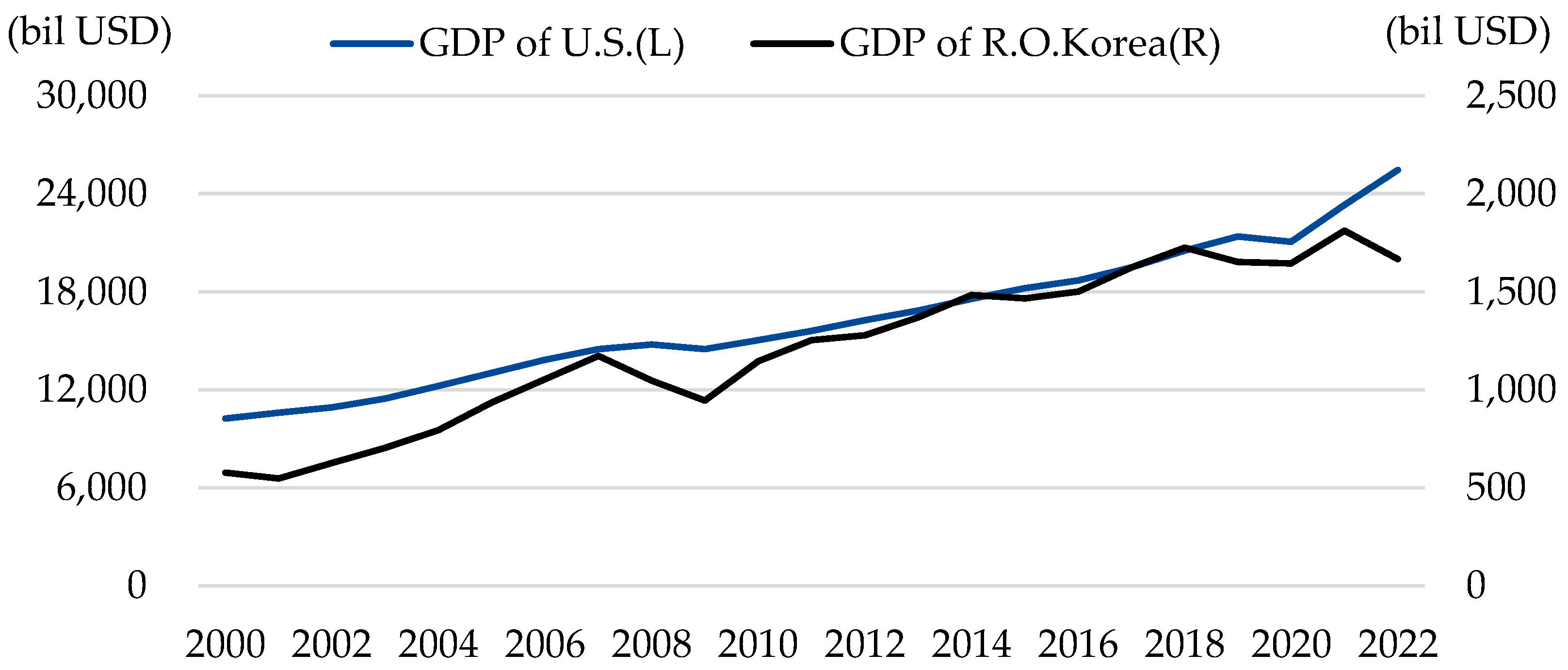
Figure 1 that the two representative indices of the U.S. and Korea have had a good record of growth as developed and emerging markets. In
Figure 2, the capitalization growth of the U.S. and Korean economies and stock markets in the recent two decades is presented, and the fundamental observation is that growth can be a foundation for market investment.
2.4. Performance Measurement Tool
The first, simple performance measurement that can be used is a stock market index chart compared with the algorithm model in the investment period. The representative measurement is a Sharpe ratio (
Sharpe 1994). This measurement ratio can compare two or more investment portfolios, including their return and volatility. The Nobel Prize-winning economist William F. Sharpe developed this tool. The Sortino ratio (
Rollinger and Hoffman 2013) measures the risk-adjusted return of a portfolio. It penalizes both upside and downside volatility equally. The Sharpe ratio measures returns falling below the expected situation. The Treynor ratio (
Van Dyk et al. 2014;
Treynor and Mazuy 1966) measures the returns earned in excess of that which could have been earned on an investment with no diversifiable risk.
Jensen’s (
1968) alpha determines the abnormal return of a portfolio over the theoretical expected return.
= asset return
risk-free return
E[ expected value
standard deviation
These are expert performance measurements used by mutual funds and institutional investors to reach the benchmark.
However, the prevenient performance measurement tools are unsuitable for “low-frequency trading” for small investors and longer-term investment periods. In these situations, we can also use the hit ratio (
Leung et al. 2000), which is the ratio of wins to losses in trading periods or whole trading actions (buying and selling).
In terms of investment, small investors struggle to cope with the high volatility of the stock market and the low hit ratio. However, an institutional investor’s strategy can use a low hit ratio and high return or high-frequency trading and volatility.
= number of successes
= number of fails
When investing over time, trading has a drawdown for an investment period, and we considered the percentage of the maximum drawdown (
Topiwala 2023b) in the total period.
Furthermore, we focused on two measurement tools, namely the return, represented by the annual return (AnnR), and the loss, represented by the maximum drawdown (MaxD). Applying this, we used ARM ratio = AnnR/MaxD (ARMR) (
Topiwala 2023a), which has also been referred to as the RoMaD (
Chen 2020).
Also, we introduced Co-MaxD(1 − MaxD) and PARC = Annr × (1 − MaxD), which are efficient and straightforward performance measurements (
Topiwala 2023a).
Two of these measurements are superior in establishing the result and are better than the Sharpe ratio (
Topiwala and Dai 2022).
From the point of view of low-frequency trading and long-term investment, the goal of investment is to maximize total return, annualized return, and the hit ratio and minimize the maximum drawdown during the investment period, while maximizing the ARM ratio and PARC.
2.5. Rule-Based Algorithm Trading Using Two-Channel Signal Indicators
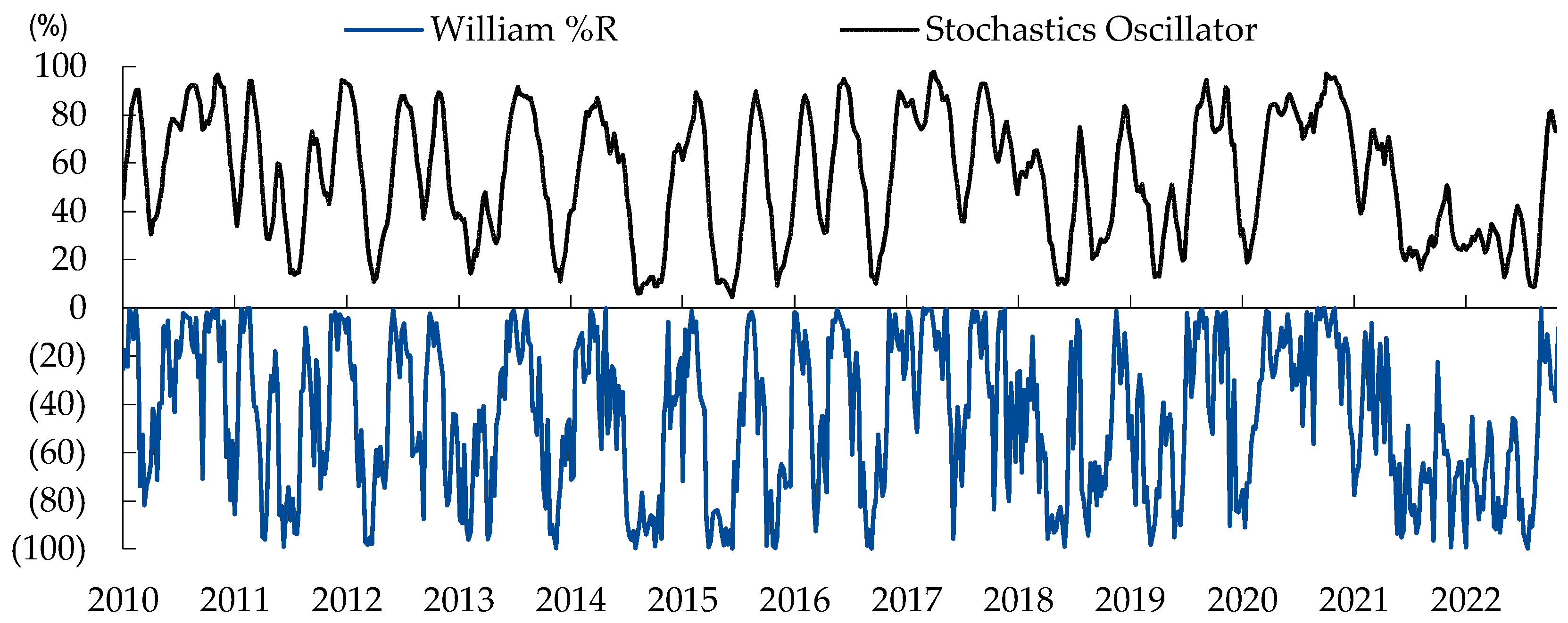
The stochastic oscillator is a representative stock market technical trading signal indicator. The stochastic oscillator (
Lane 1985) is a momentum indicator that uses support and resistance lines. The stochastic oscillator refers to the point of a current price in relation to its price range over a period (
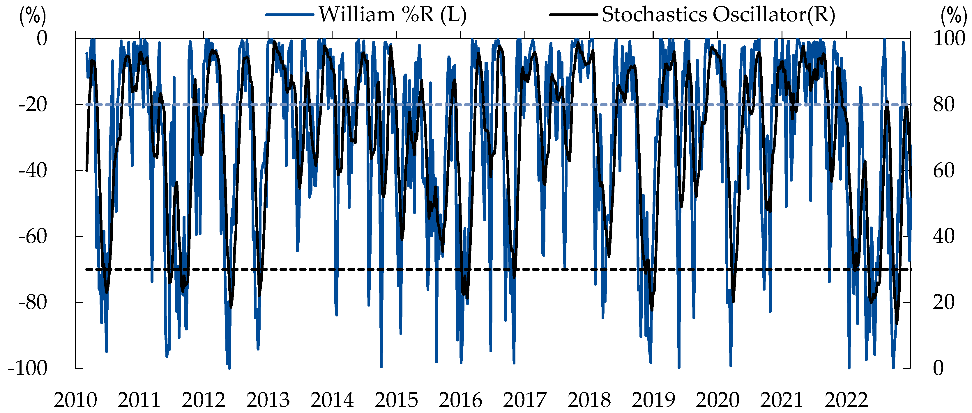
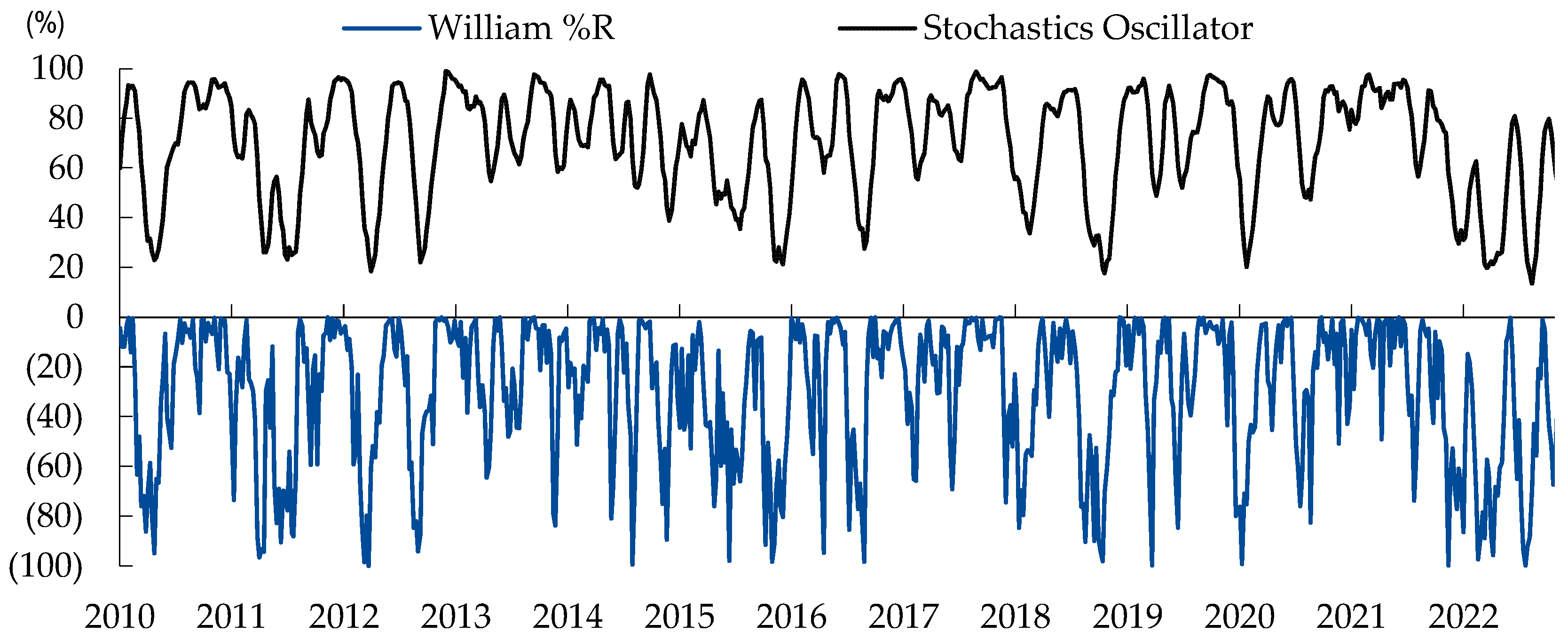
Markus and Weerasinghe 1988). The stochastic oscillator attempts to predict price turning points by comparing the closing price in the price range. We presented the equitation of the stochastic oscillator. First of all, we set the parameters for %K. We tested various n data from one to fifty-two based because we used the weekly base data. Moreover, we established that ten was fitted for n. Next, we selected the n of the %D. We tested the same data as before and selected number six for the n of the %D. The stochastic oscillator ranges from 0 to 100. A lower number for the stochastic oscillator indicates a low stock price and a higher number indicates a high stock price. We used grid searching for testing by varying the parameters by 5 units. We used ten days for %K and six numbers of %K for %D. This model recognizes the indicator value above 80 as a sell point and below 30 as a buy point.
Price = the last closing price
= the lowest price in the last n periods
= the highest price in the last n periods
%D = the n − period simple moving average of %K
%D-Slow = the n − period simple moving average of %D
In addition, the William%R is also a crucial technical signal index (
ChartSchool 2022;
Williams 2011). We chose William%R because we used the result of various oscillator tests, and it can eliminate noise signals. It helps in identifying overbought and oversold conditions on the market, which can signal potential reversal points (
Williams 2011). Similar to the stochastic oscillator, it is an indicator of where today’s market price is relative to the range of prices that have occurred during the application period. For the William%R oscillator, we tested various n data from one to fifty-two because we used the weekly base data. Moreover, we established that ten was fitted for n of the
and
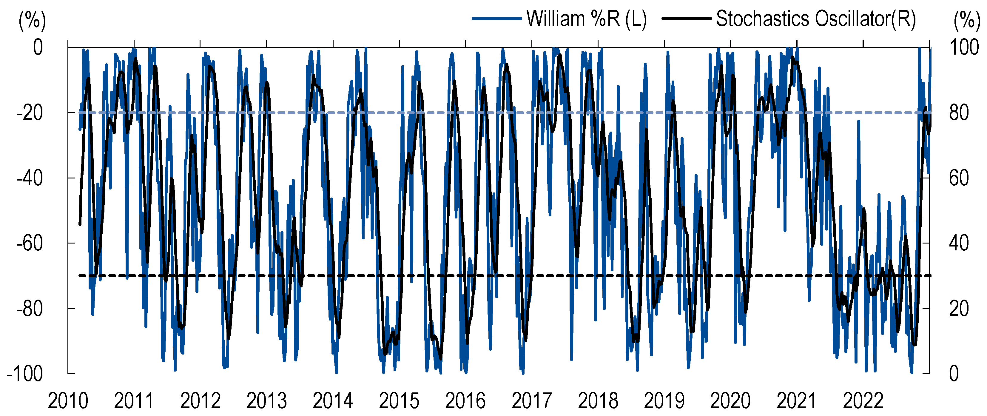
. A lower number for the William%R oscillator indicates a low stock price, and a higher number indicates a high stock price. The indicator will have a value between −100 and 0, representing the oversold range at values between −100 and −75 and the overbought range at values between −20 and 0.
Price = the last closing price
= the lowest price in the last n periods
= the highest price in the last n periods
However, sometimes, the stochastic oscillator or William%R shows the wrong signal, and this is referred to as noise—for example, when there was no buy signal previously, but sell signals appear sequentially.
First of all, predicting the stock market using the stochastic oscillator has been widely discussed in academia (
Mariani and Tweneboah 2022;
Davies 2021;
Neely 2010;
Bartolozzi et al. 2005). When the stochastic oscillator trading signal is combined with William%R, we can eliminate noise and seize the opportunity to correct the buy and sell signal. We tested various representatives of stock market technical oscillators, such as William%R, Bollinger band, MACD, MA, Envelope, RSI, Pivot, etc. The William%R technical oscillator can eliminate the noise and increase the hit ratio when used with the stochastic oscillator. The combined technical signal (stochastic oscillator and William%R), which we call
DeepSignal, reduces the failure signal (noise) and achieves beneficial results. The stochastic oscillator ranges from 0 to 100, and the William%R ranges from −100 to 0. We tested all five changed parameters to determine decisions. Moreover, we figured out which parameters were optimized. Finally, we established a standard for the algorithm’s trading rules: 1. Buy = stochastic oscillator < 30 and William%R < −75. 2. Sell = stochastic oscillator > 80 and William%R > −20. 3. Else, be cash.
We grounded our study based on the fixed rule-based trading model (
Topiwala 2023b) because it provides a straightforward approach for all kinds of investors and all degrees of freedom we tested. The prior test used a moving average for the algorithm; however, we used different oscillators. We also found that stochastic and William%R oscillators provided better results than the original indices, eliminating noise signals, reducing trading times, and lowering the maximum drawdown.
We applied a loss-cut rule to our investments to limit unexpected losses in the future. In fact, institutional investors and individual investors have loss-cut rules based on their investment goals and fund types. During the test period, the maximum drawdown of the S&P 500 was −15.1% weekly, and the maximum drawdown of the MSCI Korea was −12.3% weekly. In order to manage the investment within this more minor loss, we added a −10% weekly loss-cut rule.
Our specific algorithm suggested in this paper is described in Algorithm 1.
Furthermore, in the simulation trading results below, we provide a table and chart for the trading when the buy and sell signals are based on our trading algorithm.
The reader can test the historical index data and confirm the reported trading performance based on our algorithm trades.
| Algorithm 1: Trading algorithm. |
1. Buy = stochastic oscillator < 30 and William%R < −75.
2. Sell = stochastic oscillator > 80 and William%R > −20.
3. Else, be cash. |
3. Algorithmic Trading with Two Indices for the U.S. and Korea
We applied the thesis idea to trade with two indices: the S&P 500 and the MSCI Korea. The S&P 500 is a representative index of the U.S. stock market and a famous benchmark; in the Korean stock market, the MSCI Korea is the most famous index for foreign investors to invest in Korea. These two indices have enough historical periods for tracking and applying our low-frequency trading algorithm. We traded ETFs instead of indices for the purposes of tracking the simulation transaction. The SPY tracks the S&P 500, and the EWY tracks the MSCI Korea from January 2010 to December 2022; we studied the 144-month closing price of two ETFs. We brought the index price data from the Yahoo finance site (
https://finance.yahoo.com (accessed on 20 December 2023)), which are historically low, high, and start and end prices during the test period.
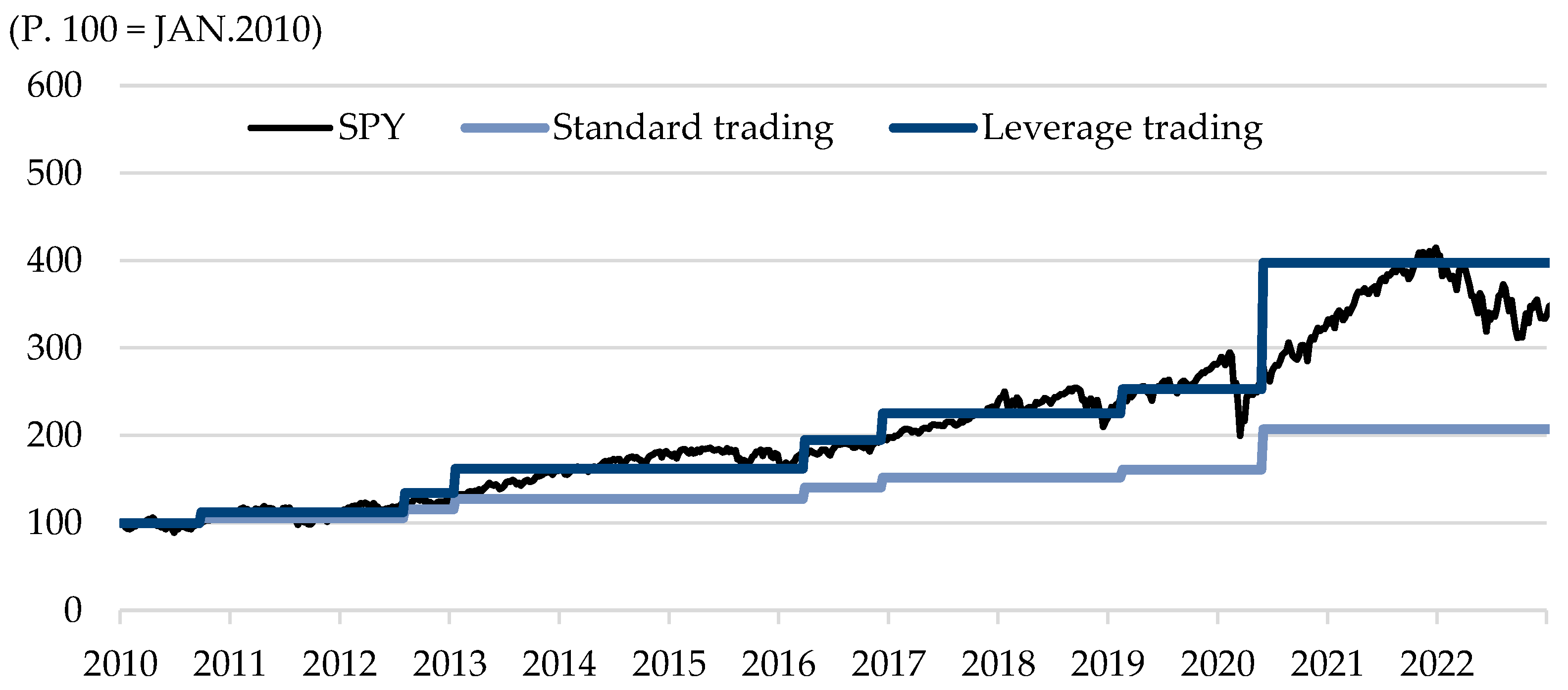
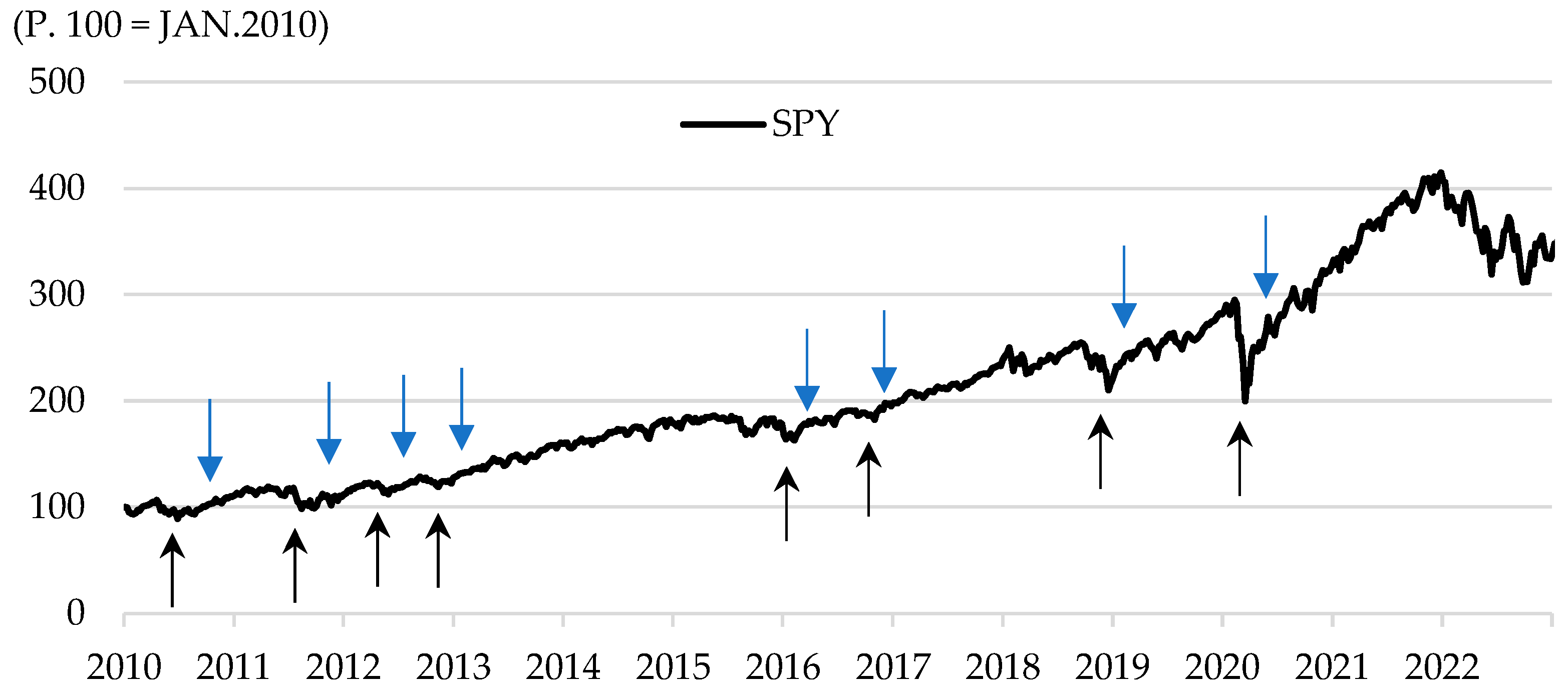
Figure 3 shows the line chart of the SPY ETF and the DeepSignal model results. This model can control the fine-tuned parameters of the stochastic oscillator and William%R and establishes standard periods (daily, weekly, monthly, etc.). However, finding an optimized performance method was not our goal. Our model focuses on clear and straightforward index trading; thus, low-frequency trading is safe for small investors.
We traded in two ways: first, trading separately and independently of each index (S&P 500, MSCI Korea), and, second, testing combined indexes such as MSCI ACWI. The S&P 500 index is a large representative index in developed markets, and the MSCI ACWI index is a representative index in emerging markets. We compared these two indices in the same investment periods. Also, the combined index would be even better if it was an independent index.
So, we examined our algorithm for each index and combined the index for low-frequency and simple trading. As a result, we did not follow the modern portfolio theory and we traded without rebalancing. As stakeholders may be novice individual stakeholder, we designed the model for their easy access and understanding. So, we used original stock market data and prices instead of using the curve fitting technique. We combined the fixed rate of the S&P 500 (80%) and the MSCI Korea (20%).
3.1. The Case of Trading with the S&P 500 Index
We chose the US S&P 500 index as our first index to apply algorithmic trading. Note that we invest in two ways: without leverage investment (called standard investment, ×1) and with leverage (×2) investment at the long (buy) position. Moreover, we did not leverage the position at the short (sell) position. Also, we never used variable multiplier leverage or the inverse. We used a fixed number (×2) leverage long position when we bought the S&P 500, and without trading, we held the cash.
We present the results of the S&P 500 algorithm trading performance in
Figure 3. In 12 years (JAN.2010~DEC.2022), we traded the SPY ETF eight times, the number of gains was eight, and the number of losses was just one, so the hit ratio was 87.5%, the maximum drawdown was −0.1%, the maximum gain was +28.7%, the leverage maximum drawdown was −0.2%, and the leverage maximum gain was +57.3%.
We compared the results with an original S&P 500 index point weekly. In 12 years, the S&P 500 grew by +244.3% (1115.1 pt to 3839.5 pt). The maximum drawdown was −15.0%, and the maximum gain was +12.1%. In light of these factors, our algorithm offers greater comfort and lower risk for low-frequency trading for small investors.
We present the simulation of the SPY ETF, which is a representative S&P 500 index. In the table below, the first buy trading signal was on 20 June 2010. On that day, the stochastic oscillator was 26.0 points, and William%R was −94.4 points in
Figure 4 and
Figure 5. After that, we followed the algorithm rule. Eight trading signals appeared in
Figure 6. The maximum gain was +28.7%, and the maximum drawdown was −0.1%. For all trading and specific oscillator numbers, see
Table 1 below.
3.2. The Case of Trading with the MSCI Korea Index
In this section, we apply our algorithmic trading strategy to the MSCI Korea index, as for the S&P 500 previously. We invested in two ways: without leverage investment (standard investment, ×1) and with leverage (×2) investment at the long (buy) position. Moreover, we did not leverage the position at the short (sell) position. We used simple and fixed multipliers when we traded the index.
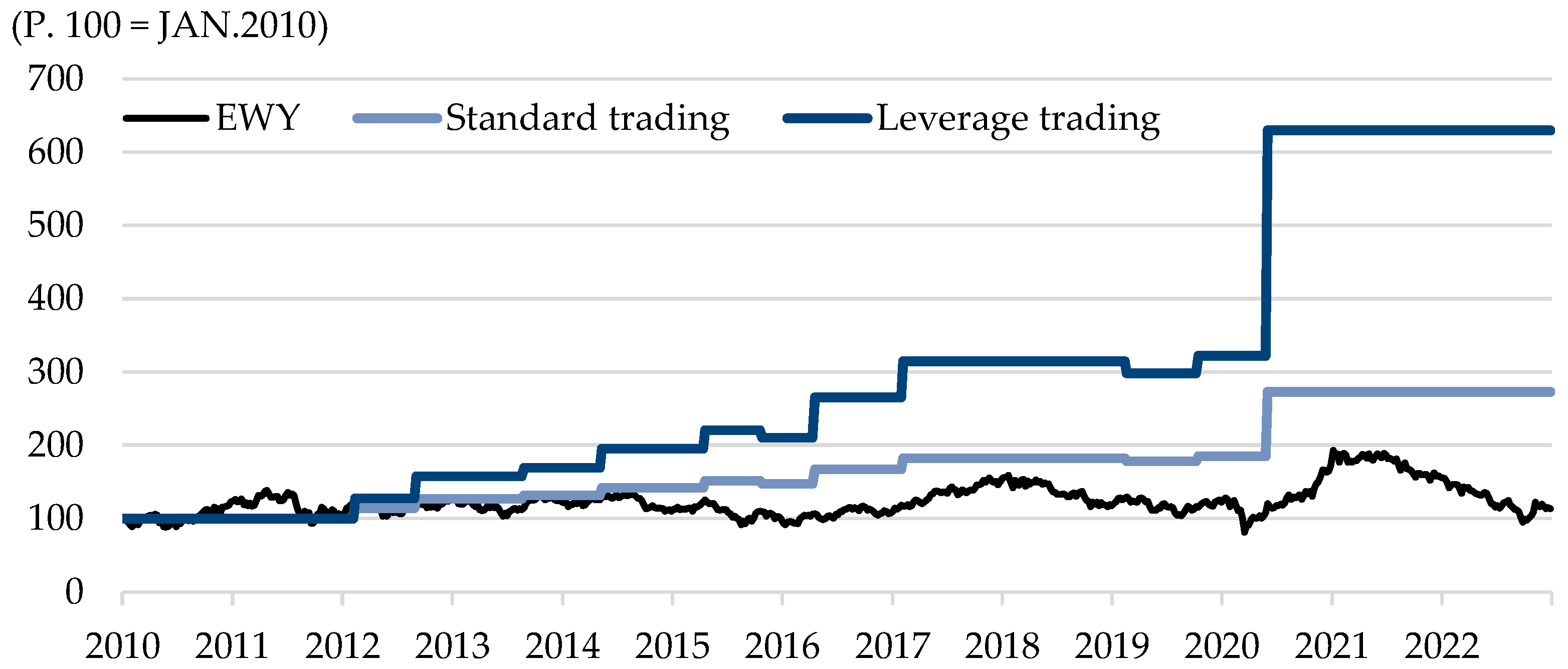
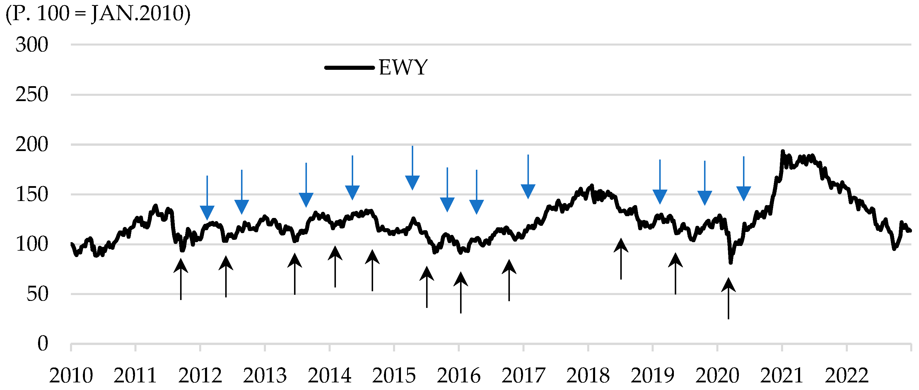
We present the results of the MSCI Korea algorithm trading performance in
Figure 7. In 12 years (JAN.2010~DEC.2022), we traded EWY ETF eleven times, the number of gains was nine, and the number of losses was two, so the hit ratio was 81.8%, the maximum drawdown was −2.5%, the maximum gain was +47.8%, the leverage maximum drawdown was −5.1%, and the leverage maximum gain was +95.6%.
We compared the results with an original MSCI Korea index point weekly. In 12 years, the MSCI Korea grew +39.5% (480.8 pt to 670.5 pt). The maximum drawdown was −12.3%, and the maximum gain was +10.4%. Regarding these factors, our algorithm offers more comfort and lower risk in low-frequency trading for small investors.
We present the simulation of the EWY ETF, which is a representative MSCI Korea index. In the table below, the first buy trading signal was on 05 September 2011. On that day, the stochastic oscillator was 14.5 points, and the William%R was −88.0 points in
Figure 8 and
Figure 9. After that, we followed the algorithm rule. Eleven trading signals appeared in
Figure 10. The maximum gain was +47.8%, and the maximum drawdown was −2.5%. For all trading and specific oscillator numbers, see
Table 2 below.
3.3. The Case of Trading with Combined Indices
In this section, we trade each index separately, but we apply different weighted portfolios of the S&P 500 and MSCI Korea. We suggested using the U.S. and the Korean markets at a proportion of 80% and 20%, respectively. This weighting reflects the MSCI ACWI, the most famous benchmark of mutual funds and developed market. The assumption of the weight of each country is based on the MSCI ACWI’s DM (developed market) and EM (emerging market) weights. The MSCI ACWI is the most commonly used benchmark for global investors. The composition of the MSCI ACWI is 80% for DM and 20% for EM for the long-term period of two decades. So, we set the DM (S&P 500) and EM (MSCI Korea) at an 8:2 ratio.
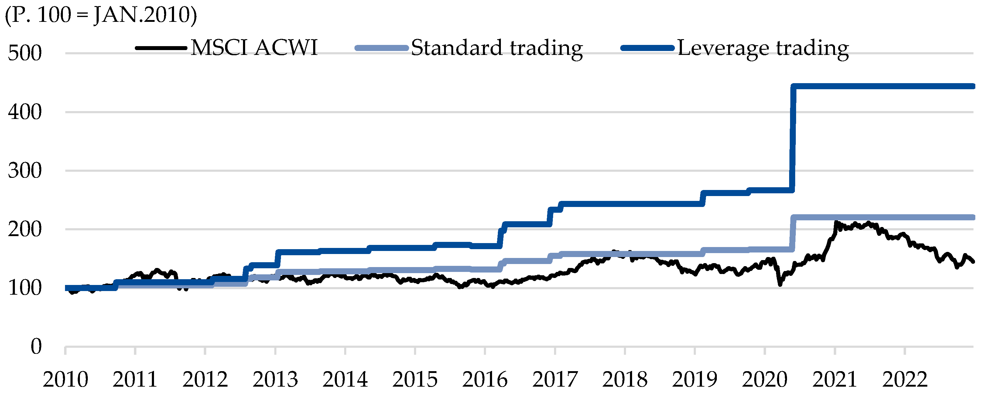
We present the results for the combined indices algorithmic trading performance in
Figure 11. In 12 years (JAN.2010~DEC.2022), we traded SPY ETF and EWY ETF nineteen times, the number of gains was sixteen, and the number of losses was three, so the hit ratio was 84.2%, the maximum drawdown was −0.5%, the maximum gain was +22.9%, the leverage maximum drawdown was −1.0%, and the leverage maximum gain was +45.8%.
We compared the results with an original MSCI ACWI index point weekly. In 12 years, the MSCI ACWI grew by +102.2% (299.4 pt to 605.4 pt). The maximum drawdown was −12.4%, and the maximum gain was +10.5%. Regarding these factors, our algorithm offers greater comfort and lower risk for low-frequency trading for small investors.
4. Discussion
We present the key findings of this study in the tables below. We separate our results into the U.S., Korean, and combined index (see
Table 3,
Table 4 and
Table 5 below). A better hit ratio was observed for U.S. trading than Korean market trading, along with lower trading times. Also, the maximum drawdown factor was better. However, the Korean market was slightly better in terms of the total return.
We calculated that the SPY (S&P 500) algorithm trading had an 87.5% hit ratio, and the EWY algorithm trading had an 81.8% hit ratio. We consider avoiding failure in trading. In both markets, we reached the goal for this. The hit ratio reached the goal by obtaining low values.
From the maximum drawdown point of view, we presented improved results, with values below mid-single digits. In the period of SPY ETF trading, the algorithm standard trading had only one negative result of −0.1%; in the case of EWY ETF trading, the maximum drawdown is just −2.5%. The scale of maximum drawdown is essential to individual and institutional investors. When the trading or investing investor has a loss-cut rule, the loss-cut standard is usually between −10 and −20% in the field. When we used our algorithm, we did not touch the loss-cut line.
The maximum gain is different, too; the SPY ETF algorithm’s maximum gain was +28.7%, lower than the EWY ETF’s +47.8%. The gap was 19.1% between the two ETFs.
Regarding the total return, the EWY (MSCI Korea) ETF algorithm leverage trading in the same test period was better than SPY ETF trading. The EWY ETF leverage trading’s final gain was +529.5%, while the SPY ETF leverage trading final gain was +297.7%, so the EWY trading’s gain was +231.8% higher.
We observe that more stable results were obtained in the combined indices case than in the case of independent index trading. The resulting values were as follows: the leverage trading total return was +344.0% (EWY case: +529.5%, SPY case +297.7%), the maximum drawdown was −1.0% (EWY case: −5.1%, SPY case −0.2%), and the hit ratio was 84.2% (EWY case: +81.8%, SPY case +87.5%). The case of combined indices improves the maximum drawdown and volatility, while combining the results of the hit ratio and total return.
5. Conclusions
We tested algorithmic trading according to rule-based market timing using a stochastic oscillator and William%R. First of all, predicting the stock market using the stochastic oscillator has been widely discussed in academia (
Mariani and Tweneboah 2022;
Davies 2021;
Neely 2010;
Bartolozzi et al. 2005). We combined the oscillators to obtain better results or to avoid risk. We tested various representatives of technical oscillators for the stock market, such as William%R, Bollinger band, MACD, MA, Envelope, RSI, Pivot, etc. The William%R technical oscillator could eliminate noise and increase the hit ratio when used with the stochastic oscillator. We achieved positive results in the global stock market over a long period. We concentrated on avoiding overfitting, which meant overtuning past data, which is common in algorithmic and quant trading. For this goal, we limited the tunable parameters as much as possible. We succeeded in fixing our parameters during the whole trading period. Using this approach, we found that our algorithmic trading provided positive results. Trading via combined indices provided better results, as shown in
Table 5. We traded two ETFs individually, but we also established the combined 8:2 ETF portfolio. Our DeepSignal model provides a strong return, a low-frequency trading signal, a high hit ratio, and a low maximum drawdown (leverage investment, 13.2% annual return, and only −1.0% maximum drawdown). These results suggest improved results for investors in active funds. The test period included the 2011 Southern Europe crisis, the 2015 interest rate increase meltdown, the economic tightening in 2019, the COVID-19 pandemic, and the 2022 stock market meltdown. Furthermore, trading was limited to six times yearly but only eight to eighteen times in 12 years by each ETF. The trading times were affordable for small investors, individual investors, and long-term institutional investors. The outcomes of this research challenge the prevailing approach of the modern portfolio theory, high-frequency trading, and the stay-in-market strategy.
We achieved optimal results for this study through limited historical optimization. We advised that the results may vary when investing in the future using this algorithm. The statement is clear about past analysis potentially not being able to guarantee future investment performance. However, instances have been confirmed where no trading occurred or losses were minimized, particularly in extreme volatility or severe annual declines. Furthermore, investment based on market timing was possible through indicators in the random path of the stock market. As a result, our algorithmic trading strategies can outperform long-term-only strategies.
We verified that our method is valid in an uptrend market, such as the S&P 500, and a sideways trend, such as the MSCI Korea. In the global stock market, the U.S. index is the representative index with the highest market capitalization, maintaining the MSCI DM upward trend during the test period. Among many indices that move sideways, the Korean index is the leading index in the EM stock market. Although we cannot generalize our findings, we consider it positive that we have achieved good results in markets with different trends.
This research resulted in the following benefits for stakeholders in the stock market. From an individual investor’s perspective, the model is able to reduce transaction costs by reducing the number of transactions. The model’s higher hit ratio and lower loss ratio can help these investors maintain stable investments. From an institutional investor’s perspective, our model enables them to maintain a stable portfolio and trade effectively as they are able to obtain better returns compared to the index and the low maximum drawdown. From an academic perspective, this study contributed methodologically to the literature by showing how to add a new oscillator to the existing trading technique that utilizes the stochastic oscillator. Infrequent trading, a high hit ratio, and better returns versus the index were obtained. This allows us to address transaction costs for real investors, allowing them to make profits and feel secure.
Furthermore, our model uses market timing effectively and provides low-frequency buy and sell signals. In the stock market conventions, market timing is impossible. We are confident that our method will be vindicated and that trading based on market timing will become possible. In a capitalist world, inflationary pressure exists, so the price (including stocks) generally rises. Our trading model can assist investors who want strong returns in low-frequency trading and limits the maximum drawdown. Additional studies could provide valuable insights into volatility, volume, and rates.


