
Revisiting Stock Market Index for the Helsinki Stock Exchange 1912–1981


Turku School of Business, University of Turku, 20014 Turku, Finland
J. Risk Financial Manag. 2024, 17(3), 90; https://doi.org/10.3390/jrfm17030090
Submission received: 17 January 2024
/
Revised: 15 February 2024
/
Accepted: 17 February 2024
/
Published: 20 February 2024
(This article belongs to the Special Issue Empirical Research on Asset Pricing and Portfolio Selection)
Abstract
:Stock market indices play a central role in portfolio and risk management and performance evaluation, as well as academic research. This paper presents a fully updated and extended stock market index for the Finnish stock market using new and updated historical databases that cover the period from the establishment of the Helsinki Stock Exchange in October 1912 to the end of 1981. In addition to the all-share market index, four industry indices are presented for the first time. The observed geometric mean market return is 1.034 percent per month (13.14% p.a.). Of the industry indices, the banking sector performed the worst as it was found to have clearly lagged behind in the market, whereas the paper and forest and the metal and manufacturing industries performed the best during the sample period. The results also highlight the importance of taking into account corporate capital actions—which are, historically, often the hardest information to obtain—as they can have a material effect on the index performance.
JEL Classification:
G32; N241. Introduction
Stock market indices play a central role in portfolio and risk management, investment evaluation, and academic research. The availability of long-term indices is of special importance for risk management as longer sample sizes allow for more accurate measurements of the risk. Similarly, they also allow for studies on long-horizon investing and on the issue of time diversification (c.f., Jorion 2003). As such, several researchers have collected data and created historical stock market indices for different markets (see, e.g., Annaert et al. (2012); Frijns and Tourani-Rad (2016); Goetzmann et al. (2001); Le Bris and Hautcoeur (2010)).
In this study, a new long-term stock market index was created for the Helsinki Stock Exchange (HSE) in Finland. This new index builds on the earlier work by Nyberg and Vaihekoski (2010). The aforementioned researchers collected a database on the Finnish stock market and used it to create a monthly all-share, value-weighted, total return stock market index for Finland that, when spliced with available similar index series from 1970 to the present day, covered the entire history of the Finnish stock market.1 However, their database, and thus their index, had some shortcomings that they acknowledged in their study. Most notably, they had access to market data only from secondary sources. In addition, they did not have information on the ex-dividend months and thus they assumed them to be April. Finally, their database on companies’ capital operations lacked details.
While creating the new index, two newly established databases were utilized. First, Vaihekoski (2022) introduced a complete listing of the listed securities in the Finnish stock market, which was extremely useful for the analysis herein. Second, this study utilized a newly introduced database on the corporate capital actions in Finland, as shown in Vaihekoski (2023). It updated and augmented the database used by Nyberg and Vaihekoski with information from newly discovered sources. With the new information, one can better understand the details of the actions and adjust the index accordingly. Furthermore, one does not have to rely on market reactions alone in determining the right off months for cash and bonus issues.
In addition, a new database of stock market data was created for this study. The data are collected from the primary source—the official quotation lists of the HSE. This allows one to avoid potential mistakes in price quotes in the secondary source, and it also helps in collecting the other potentially useful information that is included on the lists. In more detail, it turns out that the stock exchange has also kept track of dividend payments, as well as of share nominal values together with their minimum trading lots.2 This is a huge improvement in data quality. The time coverage of the new index was also extended from March 1970 to the end of 1981.
The results for the newly created all-share, value-weighted market index show that the compound monthly growth rate (geometric mean simple return) for the full sample period is 1.03 percent (13.14% p.a.), and this was achieved using the baseline total return index. The subsample results were very similar to that of Nyberg and Vaihekoski for the 1912–1970M3 period. The main differences were found to take place in the April months as the dividend payments were allocated to their rightful months. As the index coverage was extended to the end of 1981, we could compare the new index for the 1970M03–1981 period with the Berglund et al. (1983) WI index, and the results were again found to be similar. Since the data behind the WI index have disappeared for the most part, the new index allows one to conduct more detailed analyses with the constituents of the index.
In addition, a similar stock market price index was created. Once the dividends were not taken into account, the price index showed a geometric mean return of only 0.60 percent per month, i.e., 5.32% p.a. lower than the baseline index. It was also evident that it is of major importance to collect information on corporate actions even if it is often the most difficult information to acquire from historical sources. As noted in Vaihekoski (2023), bonus and cash equity issues were frequently used by the Finnish companies during the sample period; as such, they resulted in a significant contribution to investor returns. Compounded monthly percentage return would have been 0.40 percent (4.94% p.a.) lower had one ignored them in the index construction.
The contribution to the literature from this type of basic research comes, to a large extent, from further uses of the created indices. As such, this study contributes to the literature on the long-term analysis of stock market development across different countries. The new market index also gives a more accurate measure of the monthly returns and their distribution; thus, it improves risk assessments of the stock market. In addition, new industry indices also allow one to take the analysis one step further and study how different industries have performed over time and under different economic conditions. Finally, the database that was created in this study also allows for a variety of other uses (e.g., the creation of size and value indices to name a few).
The remainder of the paper is as follows. Section 2 reviews the data needed for creating the stock market index and provides details about the new stock market database collected for this study. Section 3 presents the main outcome of this study, the baseline index, and compares it with the pre-existing indices for the same periods. In addition, in this study, several long-term industry indices were created for the first time for the Finnish stock market. Finally, the effect of corporate capital actions on the index is analyzed. Section 4 concludes and offers suggestions for future research.
2. Materials and Methods
2.1. Stock Market Data
Vaihekoski (2022) presented a database that shows all of the listed securities at the main Finnish stock market: the Helsinki Stock Exchange. The database contained detailed information about the listed securities, as well as their listing period (in/out). The information was hand-collected using information from primary sources, i.e., the official quotation lists.
This database of listed securities is the basis upon which a new database for this study was collected. The new database contains information on the official quotation list, most notably the quoted bid and ask offers, as well as the transaction prices and trading volumes for all listed securities from October 1912 to December 1981.3 The ending of the sample period was based on the fact that the pre-existing research databases for Finland have detailed price information for the stocks from the last day of 1981 onward.
The data are extracted manually from the quotation lists. As this research aims to create monthly indices, and as the digitalization of the data on the lists has proven to be tedious, the decision was made to collect and digitalize only month-end official quotation lists. As some of the stocks on the list were quoted only twice a week, the data for them were taken from their last trading day in each month if it did not match the month end.
This new database extends the database in Nyberg and Vaihekoski (2010) in many ways. First, the information content of the database is far greater. The old database had only bid offers collected from the newspapers, whereas the new database includes not only full pricing information and trading volume, but also information on dividends, trading lots, and the nominal values of each share. Second, the time coverage is extended by more than eleven years from March 1970 to December 1981. Besides adding securities for the new period, a few new securities–mostly issue rights that have been listed for less than a month–were added even for the parallel years as a result of the detailed coverage of the listed securities at the HSE in Vaihekoski (2022). Ultimately, during the sample period, there were 202 listed stock series, 392 listed issue rights, and 253 newly issued stock series with lower than full dividend rights for the ongoing year.
After creating the new database, its reliability was checked. First, the bid and ask offers were compared. If the former is higher than the latter, then it would indicate an erroneous entry in the database. Similarly, the realized prices could not be higher or lower than the offers although there may be realized prices but no official bid or ask offers. To remove any potential wrongly placed decimal dots, bid offers are compared with those in the old database. If they differ by more than ten percent, a likely typo exists in either database.4 Furthermore, the consecutive prices for any series are compared. If they differ more than 50 percent, a closer scrutiny is conducted. Finally, if a positive trading volume is observed, a price has to be also given.
As such, the new database allows researchers to conduct different types of long-term studies on the Finnish stock market. Here, the main interest is to create a new and improved stock market index for Finland. The results gave us a chance to compare the results with the old index in Nyberg and Vaihekoski (2010) for 1912–1970M03 and in the WI index by Berglund et al. (1983) (which is available from March 1970 onward).5 This WI index is widely used in stock market research on the Finnish market. When the index created here was spliced with the WI index from 1982 onward and the HSE’s official total return index that is available from the last day of 1990 onward, one can study the whole history of the Finnish stock market portfolio using a research quality index.
2.2. Other Required Data
As the goal was to calculate a value-weighted total return index, which is often the reference standard for stock market indices, we needed to also collect several additional types of data. First, we needed information on the market capitalization values for all of the listed stock series. To this end, one needs information on the number of stocks issued, which—in turn—requires information on the book equity capital of companies, as well as the nominal values of each stock. As many of the listed companies had more than one listed stock class, we also needed to collect information on how the book equity was divided between the classes, which is often quite a hard-to-find piece of information.
The database constructed by the study of Nyberg and Vaihekoski (2010) was used as a starting point. It contained the year-end values of book equity capital and the nominal value of shares for each listed stock series. The values in the database were mostly collected from the HSE’s Iron Book, but since this source includes information only from the year 1915 onward, the database was augmented and updated using the information provided in the HSE’s annual statements for 1912–1914. For this study, the data were checked and some inconsistencies were fixed. Furthermore, the book equity for insurance companies was updated to reflect the covered book equity, which typically increased from year to year. Specifically, it was typical for insurance companies to allow investors to pay the nominal equity capital in installments over a period of years, and this could continue for as long as the minimum set by the law was when the company was established. In practice, however, the investors did not pay the difference. Rather, insurance companies covered the difference by using the capital adjustments over the years. In addition, several other updates were conducted based on new information from other sources. Finally, the database was augmented with new information collected for the years 1970–1981. The main source for new information was the annually published books by Gunhard Kock on publicly listed companies in Finland (e.g., Kock 1975, 1982).
The equity capital book value is used to calculate the number of shares with the help of nominal values (i.e., the covered nominal value for insurance companies). As noted earlier, the new database extracts this information from the official quotation lists. The lists had a separate column for nominal values for each stock and if the nominal value changed, e.g., due to a split, its value was changed in the column.6 Unfortunately, as noted in Vaihekoski (2022), between February 1973 and January 1974, the quotation lists did not show the nominal values. Thus, the values before and after this period were compared. The result shows that there were no changes in the nominal values during this period; as such, the values from February 1974 can instead be used during this period.
For the whole sample period, special care was given to situations where the companies changed the nominal values mid-year as this has an impact on the number of shares and market capitalization value. The obvious reasons for the changes were (reverse) splits, but it was also quite common for the companies to increase the nominal values of their shares using their own reserve capital. There can be several reasons for increasing the nominal value. As noted in Vaihekoski (2023), an increase in the nominal value could signal management’s improved forecast for the company’s future, especially if the payout rate was kept the same. The changes might have been also motivated by tax purposes. Since the year-end values of the book equity were used in this study in the numerator throughout the following year when calculating the number of shares, one needs to thus adjust the book equity for increases in the nominal values. Here we found 258 changes by the end of the year 1981. Since 30 of them were related to splits, the rest were found to be due to companies increasing (with few exceptions) the nominal value of their shares using reserve equity capital. Through analyzing their occurrence frequency distribution over the sample period, one can see that they are quite evenly distributed over time, i.e., typically one or two companies per year. However, there are years without any changes and years when the changes are more commonplace (especially in the early 1950s).
Second, to calculate the total return, we needed information on dividends. The new database could again help us since the quotation lists have a separate column for the dividends, and these are given as percentages of the nominal value. Furthermore, there was a separate column for the year of the dividend coupon. With this information, one can take note of when the dividend was paid (the coupon year changed) and calculate the dividend in FIM by multiplying the nominal value with the dividend percentage. The only exceptions to this rule are those cases where the company decide to change the nominal value of each share (e.g., via split or pure capitalization issue) at the same time as a dividend payment was decided upon and paid.7 It is the author’s understanding that the paid dividend was ultimately based on the nominal value prior to the change. In practice, for the index, the dividend is calculated using the nominal value from the previous month (adjusted for new-to-old FIM conversion if need be) if the nominal value changed the same month as the dividend was paid.
Unfortunately, the quotation lists did not show the dividend after the year 1972, except for a few companies, since the dividend column was removed from the official quotation sheets from February 1973 onward. Thus, for the period from 1973 to 1979, missing information on the dividends was collected from annual stock market books by Gunhard Kock. He provided the exact date for the dividend payments. Typically, the dividend payments began the day after the shareholders’ annual general meeting; hence, it is also the first ex-dividend date unless the stock exchange was closed. For the years 1980 and 1981, the dividends and their timing were collected from the Helsingin Sanomat newspaper.
It is interesting to study the distribution of dividend payments across the calendar year. Nyberg and Vaihekoski assumed that the dividends were paid in April. Here, the results show that, from 1912 to 1981, a total of 3531 non-zero dividends were paid. April was, as expected, the most popular month with 39.17% of all dividend payments, which was followed by March (23.68%), May (14.56%), and February (11.75%). This goes to show that the timing of the dividend may influence the total return indices.
Third, one needs to consider the influence of corporate capital actions on investor returns and thus on the index. During the sample period, Finnish publicly listed companies were active in their equity capital operations. A variety of different actions could be found ranging from (reverse) splits to equity offerings. Vaihekoski (2023) gave a detailed description of the actions during the sample period. He also collected a database of the actions, and that database was used here to calculate the appropriate adjustments in the index calculation.
This new database has several improvements over the original database in Nyberg and Vaihekoski (2010), such as it being based on the information collected from various sources, which makes the data more trustworthy and improves the coverage of the actions. Moreover, the database includes far more detailed information on actions, which can help one to decode even the most complicated ones.8
One of the major improvements was also the fact that the new database on capital actions includes information on the timing of the action (e.g., subscription periods for the cash issues). Nyberg and Vaihekoski had access only to the year of the issue for issues before the year 1960, and the actual right off months were decided upon the price reaction. At times, if the price reaction was mild or the stock suffered from thin trading, the timing was more or less an educated guess. Unfortunately, even with the new database, the timing issue is not altogether solved as the practices changed over time. More specifically, at the beginning of the sample, cash issues were subscribed to by signing a list, and the price reaction seemed to happen after the subscription period. Later, when the HSE started to trade these rights, the price reaction was often, but not always, visible right after the beginning of the subscription period. As we are using monthly data, the length of the settlement period can also influence when the right off month takes place.9
In practice, we consider three types of actions when we calculate our indices: (reverse) splits, bonus issues, and cash issues. (For more detail on how these adjustments are made, see Nyberg and Vaihekoski (2010).) For example, for the bonus and cash issues, we calculated the theoretical exercise values for the rights and used them to calculate the adjustment factors.10 The values were calculated at month end when the right offs have taken place and the stock in question is traded without the right (issue coupon). For example, the exercise value for an issue right that is attached to a single stock in a cash issue is , where is the subscription ratio and is the difference between the ex-right price for the stock on the market and the issue price.11
For those cash issues, where newly issued stocks have a lower right on the dividend for the ongoing year, one should deduct the expected dividend difference from the market price. This typically happens if the issue took place close to the end of the year.12 Since this information was not available at the time, Nyberg and Vaihekoski (2010) did not adjust for it. Here, in using the information in the Vaihekoski (2023) database, one can add this adjustment for the cash issues. In theory, the value of an issue right is the post-issue price of the stock minus the present value of the expected dividend times the fraction of the dividend new shares entitled to minus the issue price. For example, if the newly issued stocks are entitled to a percent of the dividend for the ongoing year, the theoretical value of a right to subscribe one new stock equals , where refers to present value and refers to the next dividend payment. In practice, the present value of the expected dividend was proxied with the last known dividend, and this was adjusted for potential splits.13
There are also a few dirty issues where the issued security differs from the underlying security. The most common examples are cash or bonus issues where the company issues stocks of another class, typically with fewer voting rights. For these issues, the issue adjustment is calculated as if the issued stocks were similar to the underlying stock. Specifically, both classes typically traded at fairly equal prices. However, there were also a few issues, where the issued security was not a stock but some other security (e.g., a bond) or the issued stocks belonged to a company whose stocks were not traded at all. In these cases, the adjustments were made using the observed market price for the right (if the rights were traded at the HSE).
Finally, it was also possible to create various subindices for 1912–1981. Here, we chose to calculate industry indices—which is the first time for the Finnish stock market as far as the author is aware. For this purpose, listed companies had to be classified into different industries based on their main line of business. Currently, companies’ industry sectors are readily available from databases, but historically this was not typically the case. As such, one was often forced to utilize other available historical material (e.g., books on corporate history) to decide on the appropriate industry sector. One has to keep in mind that the main line of business can change over the years and thus the classification has to be redone at times. For companies with multiple lines of business, the choice can also be somewhat subjective. Luckily, for the sample period in question, Kock provided detailed information on company operations, and it was fairly easy to select the industry codes for the companies.
When creating industry indices, the number of listed companies and the industries they represent limit the choice of indices and how industry-specific they can be. Similarly, the longer the period and the more specific industry sector one tries to cover with the index, the more difficult it becomes as industries change and so does the number of companies listed in the stock exchange. A very narrow industry classification can lead to an index with only a few companies in the industry category in question and, at the extreme, having no stocks at all. Although one can create industry indices for shorter periods, the main focus is often on indices that cover the whole sample period. For this purpose, we selected industries that allowed us to create industry indices (almost) from the beginning of the sample period to the end. In practice, four industries were selected for closer analysis. Three of the industries, the banking industry, insurance industry, and metal and manufacturing industries, had listed companies throughout the sample period. The fourth industry, the paper and forest industry—which is historically often considered the backbone of the Finnish economy—had listed companies three months after the opening of the HSE. Vaihekoski (2023) shows the number of companies in these selected industries.
3. Results
3.1. All-Share Baseline Index
The baseline index is an all-share, value-weighted, total return monthly index based on bid offers. The index in this study, for the most part, was calculated similar to the Nyberg and Vaihekoski (2010) index (henceforth labeled as the NV index). The data for book equity was basically the same as for the NV index, with minor updates for 1912–1969 and with an extension for 1970–1981. Otherwise, however, the new index utilizes newer data on capital operations from Vaihekoski (2023), as well as the bid offers, dividends, nominal values, and information on the timing of dividends collected for this study.
There were also some differences in terms of index methodology. Table 1 summarizes the selected key attributes for the new index and compares them with those of the old NV index. The main difference was that this time search back method (i.e., the missing month-end bid offers that were replaced by the last available bid offer earlier in the month) was not used. This was performed to avoid using the data from the secondary source and to focus on true month-end values. All of the stock series were included in the index except short-lived series with lower dividend rights for the ongoing year that were born out of bonus and cash issues. This time, the book equity and thus the number of stocks was not updated due to issues until the year’s end. As before, for missing bid offer values that are due to thin trading, the zero return imputation method was used, but the adjustment for dividends and issues was performed this time without delay even if a price observation was missing.14
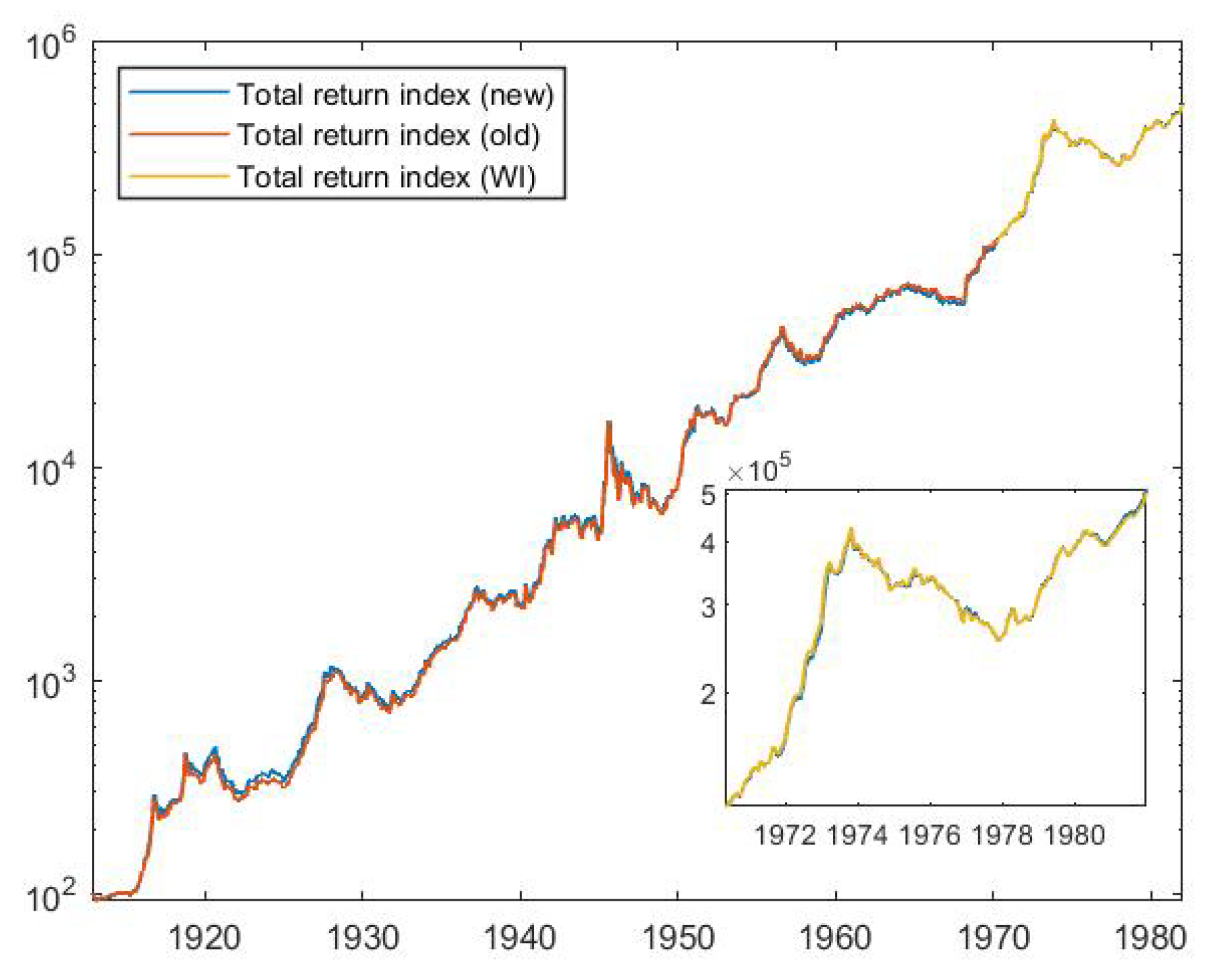
The baseline index can be seen from Figure 1. The index was calculated until the end of the year 1981. The old NV index was also included for comparison until March 1970. The base value of 100 (October 1912) was set for both. In addition, the Berglund et al. (1983) WI index was included for comparison from March 1970 onward, with the base value set to match the value of the new index in March 1970.
We can see that the indices tracked each other as one would expect. Some occasional differences were visible as the bid offers may differ from each other now and then, but the indices were found to be close to each other over time.15 Table 2 provides descriptive statistics for the percentage simple returns of the indices. In Panel A, the sample period was from October 1912 to March 1970.
The geometric mean returns, which correspond to the compound monthly growth rate (CMGR), were 1.026 and 1.027 percent (13.03% vs. 13.04% per annum) for the new and the old (NV) index, respectively. The difference was mainly driven by two opposing effects. The new index utilized detailed information on the timing of the dividend payments. This had a positive effect on the new index as close to 37 percent of the dividends were paid before April and only 24 percent after it.16 On the other hand, the decision to adjust the cash issues for the lower dividend right decreased the value of the exercise rights and thus had a negative impact on the index.
The arithmetic mean simple returns for the new and the old indices were 1.165 and 1.179 percent per month (14.9% vs. 15.1% p.a.). We tested for the significance of the arithmetic means with one-sample t-test statistics. They were found to both be significantly different from zero (as the new index t-value was 4.22). Since the test was based on the assumption that the observations are independent of each other, we re-estimated the test statistic using standard errors that were adjusted for the AR(1) process (c.f., Campbell et al. 1997). The result stayed the same—the mean return was statistically different from zero.
Volatilities were 5.44 and 5.69 percent per month for the new and the old index, respectively. The difference was likely caused by the fact that the dividend and issue right off months are now known with better precision, which removes the unnecessary volatility in returns that are caused by wrongly timed adjustments for them. A smaller impact may come from the fact that the old index used an intra-month search back method to deal with the thin trading, whereas the new index uses zero return imputations in those cases (i.e., in effect, the last bid offer is used with potential adjustments for dividends and capital actions until a new one is observed). The search back method produces more (small) non-zero returns, the latter method has more zero returns with few larger returns. The difference in methods can have either a positive or a negative impact on the index volatility depending on the return distribution.
Both series showed signs of nonnormality with positive skewness and excess kurtosis, as well as temporal dependency in the form of autocorrelation. Somewhat surprisingly, the new index had higher first-order autocorrelation (0.24 vs. 0.20). This could again be due to the differences in the way the indices deal with thin trading. In particular, using zero return imputations produces larger positive lead-lag (cross-autocorrelation) effects, which result in higher index autocorrelation (c.f., Campbell et al. 1997).
Panel B reports similar descriptive statistics for the March 1970 to December 1981 period. Since the WI index by Berglund et al. (1983) is available for this period, it is included for comparison. The geometric mean returns were 1.075 and 1.064 percent per month (13.7% vs. 13.5% p.a.), whereas the arithmetic mean returns for the new index and the WI index were 1.135 and 1.127 percent per month (14.5% vs. 14.4% p.a.), respectively. Again, both return series showed positive skewness and excess kurtosis, although to a much lower degree than before 1970. The biggest difference to Panel A was in the reduced kurtosis, which is likely to be driven by lower thin trading and leads to fewer zero returns. Both series also showed fairly high first-order autocorrelation.
3.2. Performance Analysis
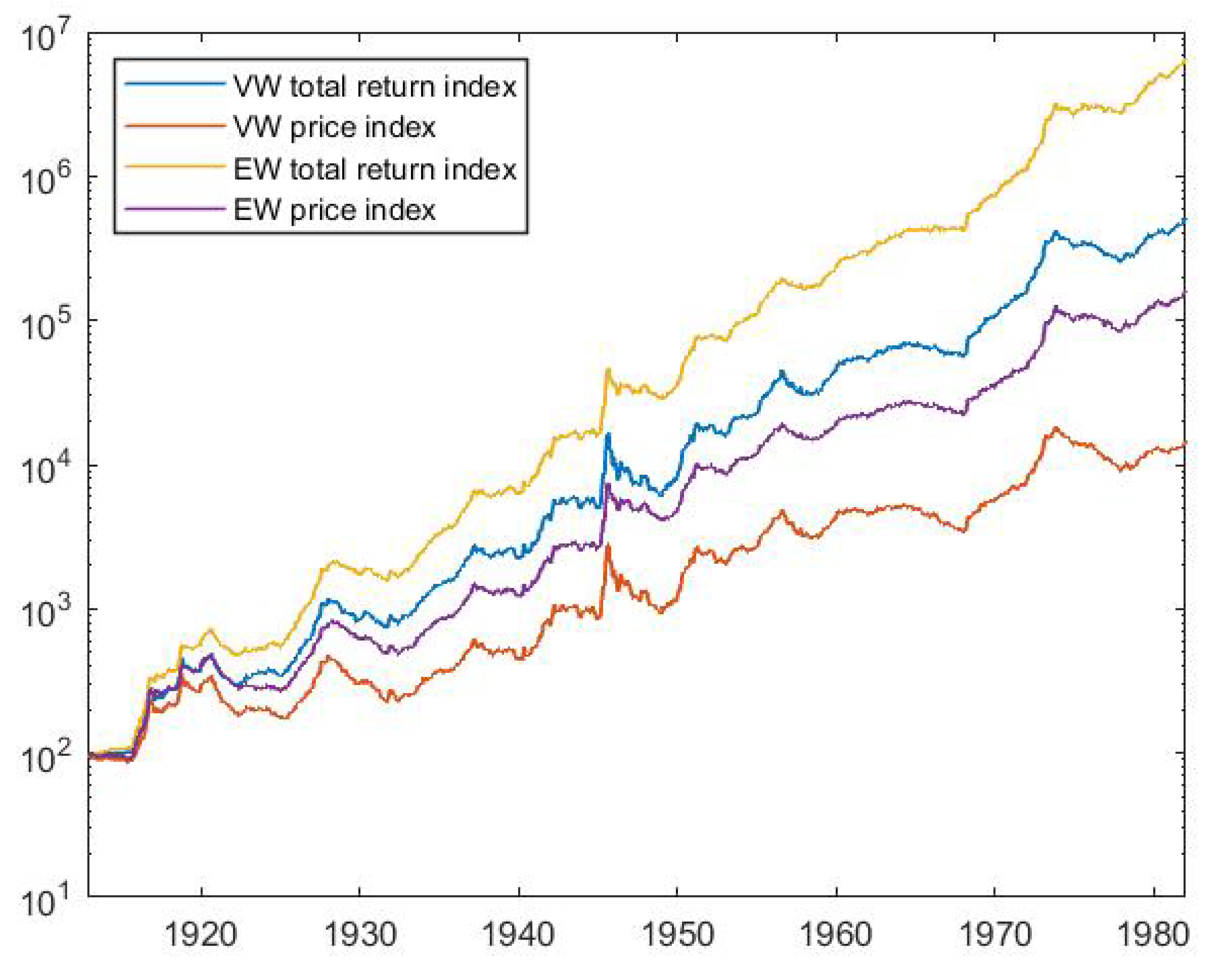
We can also analyze the impact of dividends and different capital operations on the index. To do this, we first calculated the baseline index without the dividends but also took into account capital operations (splits, bonus and cash issues). The result corresponds to the price index. Second, we re-calculate the index even without adjustments for the capital operations (except splits). This index can be labeled as the raw price index. Panel C in Table 2 reports the results for the last two indices for the full sample with the baseline index.
The geometric mean return for the total return index came down from 1.034% per month (13.14% per annum) to 0.602% (7.46% p.a.) for the price index. For the raw price index, the mean return was even lower, 0.199% (2.41% p.a.). This result highlighted the fact that—in addition to the dividends—capital operations and (especially) equity issues play a major role when creating a return index for markets where such operations are commonly used. The impact on annual returns (0.40%, 4.94% p.a.) was found to be almost as high as that of the dividends (0.43%, 5.32% p.a.).
Next, a number of different variations of the baseline index were created with different weighting structures. A natural choice is the well-known equally weighted version of the all-share indexes. Figure 2 shows the development of both value-weighted and equally weighted indices. It is clear from the figure that the equally weighted index fared much better than the value-weighted index during the sample period. This was in line with expectation as the former index gives a higher weight to smaller companies than the latter index. In addition, we calculated the book equity-weighted version of the index (not shown; available upon request). Its returns fell in between the value-weighted and equally weighted indices.
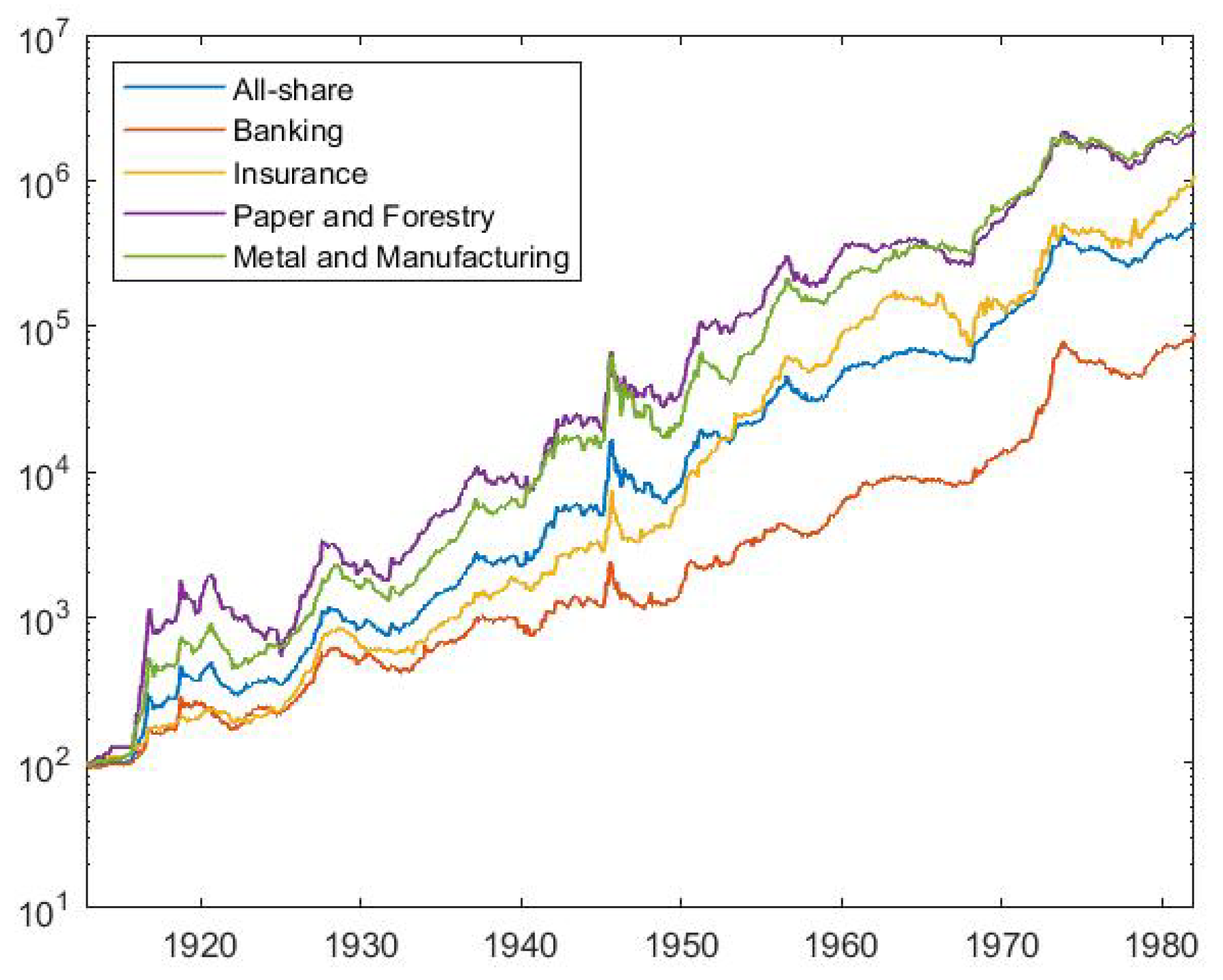
Finally, we analyzed the performance of the selected industries. Figure 3 shows the development of the value-weighted industry indices, as well as the all-share baseline market index. Panel C in Table 2 shows the descriptive statistics for the returns of the industry portfolios.
Somewhat surprisingly, the banks’ performances were found to be inferior to the general market index and the worst of the industry indices during the sample period. The geometric mean return was only 0.821 percent per month (8.99% p.a.). This could be due to the heavy regulation on the banking industry during the sample period. On the other hand, the volatility was the lowest of the three industries, which may reflect its role as a value-oriented investment during the sample period. All of the other industries fared better than the market on average. Both of the basic industries, paper and forestry and metal and manufacturing, fared the best (as one would expect given their major role in the Finnish economy during the sample period) although with much higher volatility.
3.3. Additional Considerations
It is typically the case that when one is creating a historical stock market index, the marginal cost of acquiring more information and knowledge increases during the process. At some point, one needs to consider the trade-off between the accuracy of the index and the costs of improving it. As such, it is worthwhile to discuss whether there is something that one could have been enacted to improve the index and whether it would made a meaningful difference.
In this study, three potential issues can be identified to this end. First, the indices were calculated using bid offers similar to Nyberg and Vaihekoski (2010). Of course, the bid offers can be criticized for not reflecting tradable returns. However, bid offers are observed far more frequently on thinly traded stock markets like Finland; as such, they are more likely to reflect changing market conditions.
Second, one could calculate the option value for the issue rights, which would reflect not only their exercise (intrinsic) value, but also their time value. More specifically, in most issues, investors had one or two months, and in some cases even up to six months, to exercise their subscription rights. As such, by exercising the right at the end of the right off month, we omitted the time value of the option. Similarly, in cases where the rights were traded on the market, we could have assumed that the investor sold them on the market instead of exercising them. In the end, we are, in effect, making the issue adjustment factors smaller than they should be. To analyze the situation and to see how the theoretical values compare to the prices paid in the market, we compared the theoretical value with the observed market price during the 1970s. The evidence shows that their difference was typically quite small. But, as noted earlier, there were reasons why we chose not to use either of these alternative approaches.
Third, one could have taken into account delisting returns. In particular, following most of the earlier studies, the returns for the delisting months were excluded when the index was created. The main reason for this was the difficulty in finding information regarding investor returns in delistings. For those companies that suffered bankruptcy, the selected approach clearly biases the returns upward, even though the impact is likely to be small (as the weight of these companies in the index was small before the actual bankruptcy). For the companies that were delisted as a result of the merger, including delisting returns could arguably have had a mildly positive effect on the index.
To study this issue, hand-collected data on delistings was collected for closer analysis. Altogether 136 stock series were delisted by the end of 1981, the most typical reason for delisting was mergers, which happened in 42 (30.9%) cases. This was followed by a company’s own application for delisting in 34 (25.0%) cases, a lack of enough trading in 13 (9.6%), and bankruptcy in 9 (6.6%) cases. For 18 cases, a clear reason for the delisting could not be found.
It was impossible to calculate the delisting returns in 64 of the cases (47.1%). In most of these cases, the company continued its operations as a private firm. For 22 (16.2%) cases, the delisting could have been calculated in theory but we could not retrieve enough information to calculate them. For 9 bankruptcies, the delisting return was assumed to be −100%. For the remaining 40 cases (29.4%), the delisting return could be calculated. Typically, the old owners of stocks were given new stocks in another company. Using the market price of stocks in this other company, we can derive the delisting return for these cases. On average, the return was 38.7% when bankruptcies were excluded, and 12.7% when they are included. Overall, using delisting returns in the index construction would probably improve the accuracy of the constructed index, but the impact on the returns would likely be minor and, if anything, positive.
4. Discussion
This paper presents an updated all-share, value-weighted, monthly market index for the Helsinki Stock Exchange, i.e., the main stock exchange in Finland, covering the period from its establishment in October 1912 onward. This index supersedes the old index of Nyberg and Vaihekoski (2010), as well as extends the old index by almost twelve years longer (until the end of 1981). The new index uses a new database collected for this study from primary sources and the information on official quotation lists instead of the secondary sources used for the old index. Several benefits emerged from the use of the new database. Most notably, one is now able to use the actual dividend right off months for assets, which allows us to measure the distribution of the returns more accurately. In particular, the volatility and temporal dependence of the return series were influenced by the change.
The new index also utilized the newly collected database on corporate capital actions in Vaihekoski (2023). The amount of detail on the capital actions was found to be superior to that available for the old index. As such, it helps to more accurately measure the impact of the actions on the index. Overall, the results highlighted the fact that corporate capital actions have a major impact—one comparable to that of the dividends—on the indices and thus on investors’ returns. In markets like Finland—where cash and bonus issues were more frequently used during the sample period—stock prices, even when augmented with dividend data, were not enough to provide good estimates for the realized returns.
Besides the all-share baseline index, four industry indices were also created for the first time. There were clear differences in the different industries’ performances during the sample period. Somewhat surprisingly, of the four industries, the banking sector performed the worst during the sample period. Finally, market indices with different weighting schemes were also created. Similar to earlier studies (e.g., Bolognesi et al. 2013), an index with equal weighting far outperforms the value-weighted index on the Finnish stock market.
The new database and the new indices for the Finnish stock market can be combined with the pre-existing databases and indices that are available to researchers from the beginning of 1982 onward. The index can be used to study a number of questions ranging, for example, from industry and stock market performance to equity premium (puzzle), as well as to the benefits of cross-country diversification. The combined database on individual assets also allows one to study several interesting research questions ranging from market efficiency to asset pricing and corporate behavior. The index and the database can also be extended to cover the period before the HSE was established, as well as to create other risk factor indices. These questions are left for future research.
Funding
This research was supported by OP Bank Research Foundation, the Foundation for Advancement of Finnish Securities Market, and the Nasdaq Nordic Foundation.
Data Availability Statement
The indices presented in this article are available from the author’s website at https://users.utu.fi/moovai/ (available from 16 February 2024 onwards).
Acknowledgments
I want to thank the anonymous reviewers for their comments that have helped to improve this paper. I am also grateful to the participants at the Price Currents, Financial Information, and Market Transparency Seminar, and the 19th World Economic History Congress (WEHC 2022) for their comments on an earlier, broader version of this paper.
Conflicts of Interest
The authors declare no conflicts of interest. The funders had no role in the design of the study; in the collection, analyses, or interpretation of data; in the writing of the manuscript; or in the decision to publish the results.
Abbreviations
The following abbreviations are used in this manuscript:
| CMGR | Compound monthly growth rate |
| FIM | Finnish Markka (currency of Finland during the sample period) |
| HSE | Helsinki Stock Exchange |
| NV index | Stock market index by Nyberg and Vaihekoski (2010) |
| WI index | Stock market index by Berglund et al. (1983) |
| 1 | This index has since been used in several studies (see, e.g., Jorda et al. 2019; Dimson et al. 2023). |
| 2 | Some further benefits also emerge, namely one can now identify and collect data exactly for the last day of the month. With the newspapers, the availability of the data was occasionally dependent on their publication schedule. In addition, one is now better able to pinpoint the exact dividend payout months. Finally, a few more short-lived securities that were missing from the newspapers were found and added to the database. |
| 3 | The official quotation lists are stored as bound volumes at the Central Archives for Finnish Business Records’ (Elka). Unfortunately, the last available volume is for the year 1979. Thus, data for the years 1980 and 1981 were collected from Helsingin Sanomat, the leading daily newspaper in Finland. |
| 4 | The bid offers in the newspapers can be said to be surprisingly reliable–perhaps less than one percent of the prices were erroneous. The main reason for errors was caused by rows switching places, entries staying in the list after delisting, and a few wrongly placed decimal places. |
| 5 | The index has been updated until the end of 1990 by the Department of Finance at Hanken School of Economics. Unfortunately, the information used to create the index before 1982 has, for the large part, disappeared. |
| 6 | At times, however, the change might have been delayed. For example, the nominal values were not adjusted for the new FIM until March 1963. The old FIM was converted to a new one with a 100:1 ratio at the beginning of 1963. |
| 7 | These kinds of decisions were typically made in the annual shareholders’ meeting. |
| 8 | Some capital actions, especially if they contain compounded actions (e.g., split, capitalization, and bonus issues taking place at the same time), are quite difficult to backtrack as the amount and quality of the information reduces the longer in history one goes. |
| 9 | For example, a cash issue may have a subscription period starting October 1st, but with a three-day settlement period, the right off date is actually in September, and thus the index adjustment has to be conducted already in September, not October. |
| 10 | Note that an alternative approach would be to use the market value of the issue right, but as the rights were not always traded, especially before the 1950s, we decided to calculate the value as if the investor decided to exercise the option. Yet another alternative would be to calculate a theoretical value for the right which is basically an option, and assume that the investors were able to sell it. |
| 11 | In a simple cash issue, the rules typically state that for A stocks owned, one can subscribe to B new stocks for a price of X. Now, the subscription ratio is simply . For bonus issues, the exercise price equals zero. |
| 12 | In 351 cases out of 476 cash issues during the sample year, the newly issued stocks have lower dividend rights. In bonus issues, lowered dividend rights are far rarer. |
| 13 | As an example, we can take the cash issue of Nokia in 1926. Current shareholders were allowed to subscribe to one new for each stock they owned for FIM 2000. The new shares were entitled to two-thirds of the dividend for the ongoing year and the full dividend after that. Now, the first price observation after the subscription period ran out was FIM 4000. The dividend for the year 1925 (paid in 1926) was 18% of the nominal value of FIM 2000. As a result, the value for subscription rights for one new stock is , where we have used the last known dividend as a proxy for the next dividend payment. As in this case only one stock was needed to do the subscription, the right carried by each stock was also valued at FIM 1880. It had to be taken into account when calculating the return for the right off month. |
| 14 | To understand the difference, assume that we have a stock priced at 100. In the next period, a dividend of 10 is paid, but the price observation is missing. During the next, third period, the price is again observed at 95. Now, the selected imputation method assumes that the return is first zero which implies a theoretical price of 90. Now the return for the third period is then as opposed to assuming that the dividend is paid during the third period implying a return of . For cash and bonus issues, the theoretical ex-rights price has been calculated assuming that the value of the company increases by the amount of capital raised (none in bonus issues). |
| 15 | In fact, differences in the interim observations have only a minor effect on the end-value of a stock-specific index, ceteris paribus. Similarly, for the aggregate index, the effect is quite minimal. As the geometric mean return utilizes only the first and the last observations of the index, it should also return quite similar values. Arithmetic averages, on the other hand, may differ due to differences in the price observations. |
| 16 | The average return on April months was 5.40%, but with the new index, it is only 1.82%. |
References
- Annaert, Jan, Frans Buelens, and Marc J. K. De Ceuster. 2012. New Belgian Stock Market Returns: 1832–1914. Explorations in Economic History 49: 189–204. [Google Scholar] [CrossRef]
- Berglund, Tom, Björn Wahlroos, and Lars Grandell. 1983. The KOP and the UNITAS indexes for the Helsinki Stock Exchange in the light of a New Value Weighted Index. Finnish Journal of Business Economics 32: 30–41. [Google Scholar]
- Bolognesi, Enrica, Giuseppe Torluccio, and Andrea Zuccheri. 2013. A comparison between capitalization-weighted and equally weighted indexes in the European equity market. Journal of Asset Management 14: 14–26. [Google Scholar] [CrossRef]
- Campbell, John Y., Andrew W. Lo, and A. Craig MacKinlay. 1997. The Econometrics of Financial Markets. Princeton: Princeton University Press. [Google Scholar]
- Dimson, Elroy, Paul Marsh, and Mike Staunton. 2023. Credit Suisse Global Investment Returns Yearbook 2023. Zürich: Credit Suisse Research Institute. [Google Scholar]
- Frijns, Bart, and Alireza Tourani-Rad. 2016. The long-run performance of the New Zealand stock markets: 1899–2013. Pacific Accounting Journal 28: 59–70. [Google Scholar] [CrossRef]
- Goetzmann, William N., Roger G. Ibbotson, and Liang Peng. 2001. A new historical database for the NYSE 1815 to 1925: Performance and predictability. Journal of Financial Markets 4: 1–32. [Google Scholar] [CrossRef]
- Jordà, Òscar, Katharina Knoll, Dmitry Kuvshinov, Moritz Schularick, and Alan M. Taylor. 2019. The Rate of Return on Everything, 1870–2015. The Quarterly Journal of Economics 134: 1225–98. [Google Scholar] [CrossRef]
- Jorion, Philippe. 2003. The Long-Term Risks of Global Stock Markets. Financial Management 32: 5–26. [Google Scholar] [CrossRef]
- Kock, Gunhard T. 1975. Pörssitieto 1975/6. Osakesäästäjän käsikirja. Helsinki: Pörssitieto Ky. [Google Scholar]
- Kock, Gunhard T. 1982. Pörssitieto 1982. Osakesäästäjän käsikirja. Helsinki: Tietoteos Ky. [Google Scholar]
- Le Bris, David, and Pierre-Cyrille Hautcoeur. 2010. A challenge to triumphant optimists? A blue chips index for the Paris stock exchange, 1854–2007. Financial History Review 17: 141–83. [Google Scholar] [CrossRef]
- Nyberg, Peter, and Mika Vaihekoski. 2010. A new value-weighted index for the Finnish stock market. Research in International Business and Finance 24: 267–83. [Google Scholar] [CrossRef]
- Vaihekoski, Mika. 2022. Helsinki Stock Exchange from 1912 to 1981: Trading and listed securities. Financial History Review 29: 326–41. [Google Scholar] [CrossRef]
- Vaihekoski, Mika. 2023. Equity Issuances at Helsinki Stock Exchange 1912–1981. Unpublished Working Paper. Available online: https://ssrn.com/abstract=4577566 (accessed on 10 January 2024).
Figure 1.
Old vs. new indices. Month-end values for the new all-share, value-weighted, total return index (1912M10–1981M12), the old index (1912M10–1970M03) by Nyberg and Vaihekoski (2010), and the WI index (1970M03–1981M12) by Berglund et al. (1983). The WI index was scaled to start with the end value of the new index (a closer comparison is provided in the small inset on the lower right corner).

Figure 2.
Baseline indices. Monthly values for value-weighted and equally weighted total return and price indices.
Figure 2.
Baseline indices. Monthly values for value-weighted and equally weighted total return and price indices.

Figure 3.
Industry indices. Monthly values for value-weighted total return industry indices. The all-share baseline index is included for comparison.
Figure 3.
Industry indices. Monthly values for value-weighted total return industry indices. The all-share baseline index is included for comparison.


Table 1.
Main characteristics of the baseline index. Key characteristics of the baseline index for the Helsinki Stock Exchange. Those used in the Nyberg and Vaihekoski (2010) are shown for comparison. Short-lived securities refer to the stocks issued with lower dividend rights for the ongoing year. These series were merged with the underlying (main) series after the next dividend was paid.
| This Study | Nyberg and Vaihekoski (2010) | |
|---|---|---|
| Coverage | All share | All share |
| Sample period | Oct 1912–Dec 1981 | Oct 1912–Mar 1970 |
| Timing | Month end | Month end |
| Based on | Bid offers | Bid offers |
| Source for price data | Stock Exchange, newspapers used for 1912, 1980–1981 | Secondary (newspapers) |
| Index weights | MCAP, updated monthly | MCAP, updated monthly |
| Search back | No | Yes, intra-month |
| Return imputation | 0% | 0% |
| Delisting returns | Excluded | Excluded |
| Dividend timing | When paid | April payout assumed |
| Nominal value (NV) | Updated monthly using primary data | Updated monthly using secondary data |
| Short-lived series (SLS) | Not included | Not included |
| Book equity | Year end w/instant NV adjustments | Year end w/instant NV and SLS adjustment |
| Rights issue adjustment | Yes, w/o delay | Yes, w/delay |
| Dividend adjustment in cash issues | Yes | No |
| Dirty issue adjustment | Yes, if warrant traded | No |
Table 2.
Descriptive statistics. This table presents descriptive statistics for the monthly stock market index returns. Simple returns in percent form were used in the analysis. Zero returns were used when the stock market was closed. In Panel A, the old NV index is from Nyberg and Vaihekoski (2010). In Panel B, the WI index was created by Berglund et al. (1983). In Panel C, the results are for the full sample period. The first one is the total return baseline index. The second index ignores dividends but still corrects for corporate capital actions. The third, raw price index, ignores both dividends and all corporate capital actions except splits. The last four indices are total return industry indices similar to the baseline index. The autocorrelation coefficients significantly (5%) different from zero are marked with an asterisk.
| Variable | Mean (%) | Std. | Skewness | Excess | Autocorrelation | |||
|---|---|---|---|---|---|---|---|---|
| Geometric | Arithmetic | Dev. | Kurtosis | |||||
| Panel A: October 1912–March 1970 | ||||||||
| New baseline index | 1.026 | 1.16 | 5.44 | 1.86 | 10.96 | 0.242 * | 0.079 * | 0.033 |
| Old NV index | 1.027 | 1.18 | 5.69 | 1.83 | 10.98 | 0.195 * | 0.035 | 0.056 |
| Panel B: April 1970–December 1981 | ||||||||
| New baseline index | 1.075 | 1.14 | 3.52 | 0.51 | 2.27 | 0.247 * | 0.199 * | 0.080 * |
| Old WI index | 1.064 | 1.13 | 3.61 | 0.77 | 3.28 | 0.235 * | 0.171 * | 0.115 * |
| Panel C: October 1912–December 1981 | ||||||||
| All-share baseline index | 1.034 | 1.16 | 5.16 | 1.83 | 11.45 | 0.242 * | 0.088 * | 0.037 |
| All-share price index | 0.602 | 0.73 | 5.18 | 1.84 | 11.45 | 0.243 * | 0.084 * | 0.023 |
| All-share raw price index | 0.199 | 0.33 | 5.24 | 1.74 | 11.10 | 0.246 * | 0.063 | 0.005 |
| Banking index | 0.821 | 0.93 | 4.70 | 1.45 | 7.72 | 0.088 * | 0.103 * | 0.061 |
| Insurance index | 1.125 | 1.27 | 5.56 | 1.18 | 6.35 | 0.114 * | -0.042 | 0.005 |
| Paper and Forestry index | 1.210 | 1.46 | 7.22 | 1.60 | 8.87 | 0.179 * | 0.148 * | 0.060 |
| Metal and Manuf. index | 1.229 | 1.42 | 6.30 | 1.76 | 11.11 | 0.246 * | 0.051 | 0.066 |
Disclaimer/Publisher’s Note: The statements, opinions and data contained in all publications are solely those of the individual author(s) and contributor(s) and not of MDPI and/or the editor(s). MDPI and/or the editor(s) disclaim responsibility for any injury to people or property resulting from any ideas, methods, instructions or products referred to in the content. |
© 2024 by the author. Licensee MDPI, Basel, Switzerland. This article is an open access article distributed under the terms and conditions of the Creative Commons Attribution (CC BY) license (https://creativecommons.org/licenses/by/4.0/).
Share and Cite
MDPI and ACS Style
Vaihekoski, M. Revisiting Stock Market Index for the Helsinki Stock Exchange 1912–1981. J. Risk Financial Manag. 2024, 17, 90. https://doi.org/10.3390/jrfm17030090
AMA Style
Vaihekoski M. Revisiting Stock Market Index for the Helsinki Stock Exchange 1912–1981. Journal of Risk and Financial Management. 2024; 17(3):90. https://doi.org/10.3390/jrfm17030090
Chicago/Turabian StyleVaihekoski, Mika. 2024. "Revisiting Stock Market Index for the Helsinki Stock Exchange 1912–1981" Journal of Risk and Financial Management 17, no. 3: 90. https://doi.org/10.3390/jrfm17030090