A general derivation of the classical Doppler effect in 3D space

The classical Doppler effect is a purely kinematic phenomenon caused by the finite propagation speed of waves in media. Since waves do not propagate instantly, any signal emitted by a source reaches the receiver with some delay. If the source and/or the receiver are in motion with respect to the medium, their distance in general varies over time, and the delay varies accordingly. The variation of the delay provokes a deformation of the received wave compared to the emitted one along the time axis. In the case of periodic waves, for which a frequency can be defined, it is observed that the frequency ${\nu }^{{\prime} }$ perceived by the receiver differs from the frequency $\nu$ emitted by the source. This phenomenon was first studied by Christian Andreas Doppler in 1842, and is therefore known as the Doppler effect, or Doppler shift [1].

The topic of this paper is the classical Doppler effect between a point-like source and a point-like receiver moving with constant velocities with respect to an inertial, non-dispersive medium. More precisely, we study what happens if the source emits a periodic, spherical wave, with the same intensity in all directions, propagating at a constant speed $c.$ An example of such wave is a musical note, $c$ being the speed of sound in air. More generally, the classical Doppler effect concerns any kind of waves which can be described in terms of classical mechanics. However, we will always refer to sound waves for convenience. This way, we can avoid sentences such as ≪the receiver moves at a lower speed than the propagation speed of waves in the medium≫, stating, more briefly, ≪the receiver moves at subsonic speed≫.

To begin with, let us define the main variables that describe the source-receiver system. We call ${{\boldsymbol{r}}}_{{\rm{S}}}\left(t\right)$ and ${{\boldsymbol{r}}}_{{\rm{R}}}\left(t\right)$ the positions of the source and receiver over time, ${{\boldsymbol{v}}}_{{\rm{S}}}$ and ${{\boldsymbol{v}}}_{{\rm{R}}}$ their respective velocities and ${v}_{{\rm{S}}}$ and ${v}_{{\rm{R}}}$ their speeds. We also call ${\boldsymbol{\rho }}\left(t\right)={{\boldsymbol{r}}}_{{\rm{R}}}\left(t\right)-{{\boldsymbol{r}}}_{{\rm{S}}}\left(t\right)$ the position of the receiver with respect to the source: its norm, $\rho \left(t\right),$ is the distance between the source and the receiver, while the unit vector $\hat{{\boldsymbol{\rho }}}\left(t\right)={\boldsymbol{\rho }}\left(t\right)/\rho \left(t\right)$ is the direction of the line linking the source to the receiver. We then define ${\theta }_{{\rm{S}}}\left(t\right)$ the angle between $\hat{{\boldsymbol{\rho }}}\left(t\right)$ and ${{\boldsymbol{v}}}_{{\rm{S}}},$ ${\theta }_{{\rm{R}}}\left(t\right)$ the angle between $\hat{{\boldsymbol{\rho }}}\left(t\right)$ and ${{\boldsymbol{v}}}_{{\rm{R}}},$ and $\alpha$ the constant angle between ${{\boldsymbol{v}}}_{{\rm{S}}}$ and ${{\boldsymbol{v}}}_{{\rm{R}}}.$ An example of a source-receiver system at a given instant $t$ is shown in figure 1. Note that the vectors ${{\boldsymbol{v}}}_{{\rm{S}}},$ ${{\boldsymbol{v}}}_{{\rm{R}}}$ and $\hat{{\boldsymbol{\rho }}}$ do not necessarily lay on the same plane.

Zoom In Zoom Out Reset image size

A simple case of the Doppler effect is the longitudinal case, which occurs when the source and the receiver move along the same line, namely when the angles ${\theta }_{{\rm{S}}}$ and ${\theta }_{{\rm{R}}}$ are equal to $0$ or $\pi$ in the four possible combinations. In this case, it can be shown that

$$\begin{eqnarray}&&\frac{{\nu }^{{\prime} }}{\nu }=\frac{c\pm {v}_{{\rm{R}}}}{c\mp {v}_{{\rm{S}}}}\end{eqnarray} \tag{ 1 }$$

where the sign in the numerator is positive if the receiver moves towards the source (and negative otherwise), while the sign in the denominator is negative if the source moves towards the receiver (and positive otherwise). Equation (1) appears in several textbooks and papers [2–5], and it is known as the longitudinal Doppler effect formula.

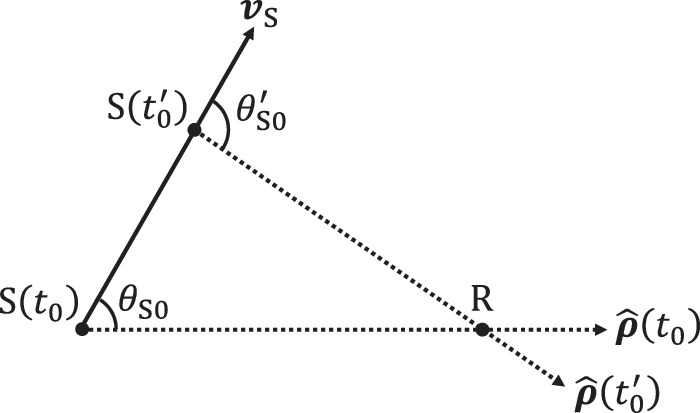
The Doppler effect in three dimensions is more difficult to describe. Due to its complexity, it is often studied in some special cases, such as the case of a resting receiver with respect to the medium. Suppose that the source emits a maximum at the instant ${t}_{0}=0$ and that the receiver hears that maximum at a later instant ${t}_{0}^{{\prime} }.$ Since sound takes some time to reach the receiver, the source moves in the meantime. Therefore, at ${t}_{0}^{{\prime} },$ the direction $\hat{{\boldsymbol{\rho }}}\left({t}_{0}^{{\prime} }\right)$ in which an observer holding the receiver sees the source does not coincide with the direction $\hat{{\boldsymbol{\rho }}}\left({t}_{0}\right)$ from which the observer hears the sound coming, as shown in figure 2.

Zoom In Zoom Out Reset image size

We will therefore call emission angle ${\theta }_{{\rm{S}}0}={\theta }_{{\rm{S}}}\left({t}_{0}\right),$ namely the angle between $\hat{{\boldsymbol{\rho }}}\left({t}_{0}\right)$ and ${{\boldsymbol{v}}}_{{\rm{S}}},$ and reception angle ${\theta }_{{\rm{S}}0}^{{\prime} }={\theta }_{{\rm{S}}}\left({t}_{0}^{{\prime} }\right),$ namely the angle between $\hat{{\boldsymbol{\rho }}}\left({t}_{0}^{{\prime} }\right)$ and ${{\boldsymbol{v}}}_{{\rm{S}}}$. The Doppler effect can be either expressed in terms of ${\theta }_{{\rm{S}}0}$ or ${\theta }_{{\rm{S}}0}^{{\prime} }.$ Textbooks usually report the formula in terms of ${\theta }_{{\rm{S}}0}$ [6–8]:

$$\begin{eqnarray}&&\frac{{\nu }^{{\prime} }}{\nu }=\frac{1}{1-{\beta }_{{\rm{S}}}\cos {\theta }_{{\rm{S}}0}},\end{eqnarray} \tag{ 2 }$$

where ${\beta }_{{\rm{S}}}={v}_{{\rm{S}}}/c.$

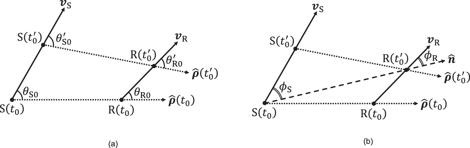
If both the source and the receiver move with respect to the medium, describing the Doppler effect is even more challenging. Since, in this case, both the source and the receiver are in motion, two emission angles and two reception angles can be defined, as shown in figure 3(a). More precisely, we call emission angles ${\theta }_{{\rm{S}}0}={\theta }_{{\rm{S}}}\left({t}_{0}\right)$ and ${\theta }_{{\rm{R}}0}={\theta }_{{\rm{R}}}\left({t}_{0}\right),$ while we call reception angles ${\theta }_{{\rm{S}}0}^{{\prime} }={\theta }_{{\rm{S}}}\left({t}_{0}^{{\prime} }\right)$ and ${\theta }_{{\rm{R}}0}^{{\prime} }={\theta }_{{\rm{R}}}\left({t}_{0}^{{\prime} }\right).$

Zoom In Zoom Out Reset image size

Note that an observer operating the source can easily measure the emission angles ${\theta }_{{\rm{S}}0}$ and ${\theta }_{{\rm{R}}0},$ as they depend on $\hat{{\boldsymbol{\rho }}}\left({t}_{0}\right),$ which is the direction where the observer sees the receiver while he is emitting the sound. Similarly, an observer holding the receiver can easily measure the reception angles ${\theta }_{{\rm{S}}0}^{{\prime} }$ and ${\theta }_{{\rm{R}}0}^{{\prime} }:$ indeed, these angles depend on $\hat{{\boldsymbol{\rho }}}\left({t}_{0}^{{\prime} }\right),$ which is the direction where the observer sees the source while he is hearing the sound. Therefore, one would expect a Doppler effect formula in terms of the emission angles or the reception angles, but such a formula has yet to be found.

A few textbooks [9, 10] report as a general formula the expression

$$\begin{eqnarray}&&\frac{{\nu }^{{\prime} }}{\nu }=\frac{1-{\beta }_{{\rm{R}}}\cos {\phi }_{{\rm{R}}}}{1-{\beta }_{{\rm{S}}}\cos {\phi }_{{\rm{S}}}}\end{eqnarray} \tag{ 3 }$$

where ${\beta }_{{\rm{R}}}={v}_{{\rm{R}}}/c.$ However, they fail to explain the meaning of ${\phi }_{{\rm{S}}}$ and ${\phi }_{{\rm{R}}}.$ In fact, ${\phi }_{{\rm{S}}}$ and ${\phi }_{{\rm{R}}}$ are neither the emission angles nor the reception angles, but the angles shown in figure 3(b), which we called hybrid angles. More precisely, if we call $\hat{{\boldsymbol{n}}}$ the unit vector linking the position of the source at the emission instant ${t}_{0}$ to the position of the receiver at the reception instant ${t}_{0}^{{\prime} },$ ${\phi }_{{\rm{S}}}$ is the angle between $\hat{{\boldsymbol{n}}}$ and ${{\boldsymbol{v}}}_{{\rm{S}}},$ while ${\phi }_{{\rm{R}}}$ is the angle between $\hat{{\boldsymbol{n}}}$ and ${{\boldsymbol{v}}}_{{\rm{R}}}.$ This is explained in two papers [11, 12], which also provide a derivation of equation (3).

Of course, equation (3) continues to hold in the case of a resting receiver or in the case of a resting source. If the receiver is at rest, ${\beta }_{{\rm{R}}}=0$ and ${\phi }_{{\rm{S}}}$ coincides with ${\theta }_{{\rm{S}}0},$ so we get once again equation (2). If the source is at rest, ${\beta }_{{\rm{S}}}=0$ and ${\phi }_{{\rm{R}}}$ coincides with ${\theta }_{{\rm{R}}0}^{{\prime} },$ so we get a Doppler effect formula for a resting source in terms of the reception angle ${\theta }_{{\rm{R}}0}^{{\prime} }:$

$$\begin{eqnarray}&&\frac{{\nu }^{{\prime} }}{\nu }=1-{\beta }_{{\rm{R}}}\cos {\theta }_{{\rm{R}}0}^{{\prime} }\end{eqnarray} \tag{ 4 }$$

The problem with equation (3) is that it is hard to apply in practice. For instance, if an observer operating the source wants to use equation (3) to get the frequency perceived by the receiver, he needs to know the direction where the receiver will be at the reception instant, namely $\hat{{\boldsymbol{n}}},$ to establish the angles ${\phi }_{{\rm{S}}}$ and ${\phi }_{{\rm{R}}}.$ However, the direction where the receiver will be at the reception instant is unknown to the observer. So, equation (3) expresses the Doppler shift in terms of two unknown angles, ${\phi }_{{\rm{S}}}$ and ${\phi }_{{\rm{R}}},$ without explaining how to determine them. At this point, there are two possible ways to compute the Doppler shift: one can either find a mathematical way to establish the angles ${\phi }_{{\rm{S}}}$ and ${\phi }_{{\rm{R}}}$ in terms of physical quantities that are known to the observer, or approach the problem in a completely new way. In this paper, we choose the second path.

First, we set a rigorous definition of the Doppler shift, which offers a kinematical way to compute it. Then, we apply the definition to the case of a moving source and a moving receiver in 3D space. This way, we get two equivalent Doppler effect formulas: one in terms of the emission angles, which can be directly applied by an observer moving with the source, and one in terms of the reception angles, which can be directly applied by an observer moving with the receiver. We also obtain two more general expressions describing the Doppler shift evolution over time. Finally, to validate our results, we compare them with the known Doppler effect formulas in some special cases.

The Doppler shift for a source-receiver system is usually defined as the ratio between the frequency ${\nu }^{{\prime} }$ perceived by the receiver and the frequency $\nu$ emitted by the source. However, such a definition can only work once the definition of ${\nu }^{{\prime} }$ is set. Unfortunately, in most cases, even if the emitted wave is periodic, the received wave is not, so it is not possible to define its frequency in the classical sense of the term. In this paper, we define ${\nu }^{{\prime} }$ as follows. Suppose that the source emits a harmonic wave of period $T.$ Suppose further that two consecutive maxima are emitted by the source at ${t}_{1}=t,$ ${t}_{2}=t+T,$ and received at ${t}_{1}^{{\prime} },$ ${t}_{2}^{{\prime} }.$ We call perceived period, ${T}^{{\prime} },$ the time interval ${t}_{2}^{{\prime} }-{t}_{1}^{{\prime} }$ between the reception of the two maxima. We then define the perceived frequency, ${\nu }^{{\prime} },$ as $1/{T}^{{\prime} }.$

At this point, it would seem natural to define the Doppler shift as

$$\begin{eqnarray}&&\mathop{{DS}}\limits^{\unicode{x0007E}}\triangleq \frac{{t}_{2}-{t}_{1}}{{t}_{2}^{{\prime} }-{t}_{1}^{{\prime} }}=\frac{T}{{T}^{{\prime} }}=\frac{{\nu }^{{\prime} }}{\nu }\end{eqnarray} \tag{ 5 }$$

with ${t}_{1}=t$ and ${t}_{2}=t+T.$ Equation (5) quantifies how shortened or stretched a single period of the emitted wave appears to the receiver. If we apply it to the longitudinal case, we get equation (1). Note that the right-hand side of equation (1) is constant. Thus, $\widetilde{{DS}}$ in the longitudinal case does not depend on the frequency of the source. This statement is by no means obvious. In fact, the problem with equation (5) is that $\widetilde{{DS}}$ depends on $\nu$ if the definition is applied to the 3D case. The reason is explained below.

According to equation (5), to compute $\widetilde{{DS}}$ we first need to establish the reception instants ${t}_{1}^{{\prime} }$ and ${t}_{2}^{{\prime} }$ of the two maxima. The reception instant ${t}^{{\prime} }$ of a maximum can be established by knowing its corresponding emission instant $t,$ the state of the source-receiver system at $t$ and the speed of sound. Let us assume that the state of the system at $t=0$ is known, as well as the speed of sound. The state of the system at $t$ can be determined from the state at $t=0$ by simply knowing the elapsed time $t.$ So, the reception instant of a maximum only depends on its emission instant: ${t}^{{\prime} }={t}^{{\prime} }\left(t\right).$ In our case, since the emission instants of the maxima are ${t}_{1}=t$ and ${t}_{2}=t+T,$ it follows that ${t}_{1}^{{\prime} }={t}_{1}^{{\prime} }\left(t\right)$ and ${t}_{2}^{{\prime} }={t}_{2}^{{\prime} }\left(t+T\right).$ Thus, the perceived period, ${T}^{{\prime} }={t}_{2}^{{\prime} }-{t}_{1}^{{\prime} },$ is a function of $t$ and $t+T,$ or simply $t$ and $T:$ ${T}^{{\prime} }={T}^{{\prime} }\left(t,{T}\right).$ By consequence, the perceived frequency, ${\nu }^{{\prime} }=1/{T}^{{\prime} },$ is also a function of $t$ and $T,$ or else $t$ and $\nu .$ Finally, since $\widetilde{{DS}}$ is equal to ${\nu }^{{\prime} }\left(t,\nu \right)/\nu ,$ it depends in general on both $t$ and $\nu .$ In some special cases, such as the longitudinal case, $\nu$ cancels out in computing the ratio. However, this does not happen in the 3D case.

The dependence of $\widetilde{{DS}}$ on $t$ is simply a consequence of the time evolution of the system: as the configuration of the system evolves, ${\nu }^{{\prime} }$ slowly changes over time, and $\widetilde{{DS}}$ varies accordingly. The dependence on $\nu ,$ on the other hand, is more problematic. For example, by applying equation (5) in the case of a resting receiver, we do not get equation (2), but a more complex expression dependent on $\nu .$ More precisely, for a sound emitted at ${t}_{0}=0,$ we get

$$\begin{eqnarray}&&\widetilde{{DS}}=\frac{1}{1+\sqrt{{{\xi }_{0}}^{2}{\nu }^{2}-2{\xi }_{0}{\beta }_{{\rm{S}}}\cos {\theta }_{{\rm{S}}0}\nu +{{\beta }_{{\rm{S}}}}^{2}}-{\xi }_{0}\nu \,}\end{eqnarray} \tag{ 6 }$$

where ${\xi }_{0}$ is the initial distance between the source and the receiver divided by the speed of sound.

If we want the Doppler shift to be a physical quantity that does not depend on $\nu ,$ we need to choose the two emission instants ${t}_{1}$ and ${t}_{2}$ very close in time. More precisely, we need to compute the ratio $\left({t}_{2}-{t}_{1}\right)/\left({t}_{2}^{{\prime} }-{t}_{1}^{{\prime} }\right)$ in the limit ${t}_{2}\to {t}_{1}.$ This way, we get a physical quantity that describes how an infinitely small portion of the emitted wave is perceived by the receiver. In short, we define the Doppler shift for a sound emitted at ${t}_{1}=t$ and received at ${t}_{1}^{{\prime} }={t}^{{\prime} }$ as

$$\begin{eqnarray}&&{DS}(t\unicode{x021DD}{t}^{{\prime} })\triangleq \mathop{\mathrm{lim}}\limits_{{t}_{2}\to {t}_{1}}\frac{{t}_{2}-{t}_{1}}{{t}_{2}^{^{\prime} }-{t}_{1}^{^{\prime} }}\end{eqnarray} \tag{ 7 }$$

where the parenthesis $(t\unicode{x021DD}{t}^{{\prime} })$ highlights the emission and the reception instants of sound.

If the state of system at $t=0$ and the speed of sound are known, the reception instants ${t}_{1}^{{\prime} }$ and ${t}_{2}^{{\prime} }$ only depend on the emission instants ${t}_{1}$ and ${t}_{2},$ and so does the ratio $\left({t}_{2}-{t}_{1}\right)/\left({t}_{2}^{{\prime} }-{t}_{1}^{{\prime} }\right).$ The limit ${t}_{2}\to {t}_{1}$ removes the dependence on ${t}_{2},$ hence ${DS}$ only depends on ${t}_{1},$ or else $t.$

At this point, some may argue that ${DS},$ despite being well defined, does not represent what is normally meant by the Doppler effect, i.e. the ratio between the frequency perceived by the receiver and the frequency emitted by the source. So, let us show why this is not true. Suppose that the source emits a periodic wave of period $T.$ Computing the ratio $\left({t}_{2}-{t}_{1}\right)/\left({t}_{2}^{{\prime} }-{t}_{1}^{{\prime} }\right)$ for ${t}_{1}=t$ and ${t}_{2}\to {t}_{1}$ is equal to computing it for ${t}_{1}=t,$ ${t}_{2}=t+T$ and $T\to 0.$ Therefore, equation (7) reads as

$$\begin{eqnarray}&&{DS}(t{\unicode{x021DD}}{t}^{{\rm{^{\prime} }}})\triangleq \mathop{\mathrm{lim}}\limits_{{t}_{2}\to {t}_{1}}\frac{{t}_{2}-{t}_{1}}{{t}_{2}^{{\rm{^{\prime} }}}-{t}_{1}^{{\rm{^{\prime} }}}}=\mathop{\mathrm{lim}}\limits_{T\to 0}\frac{T}{{T}^{^{\prime} }\left(t,T\right)}=\mathop{\mathrm{lim}}\limits_{\nu \to {\rm{\infty }}}\frac{{\nu }^{^{\prime} }\left(t,\nu \right)}{\nu }\end{eqnarray} \tag{ 8 }$$

with ${t}_{1}=t$ and ${t}_{2}=t+T.$ In other words, the Doppler shift is equal to the ratio ${\nu }^{{\prime} }/\nu$ that one would observe over time if the source emitted a sound of a very high frequency. This means that, if the actual frequency emitted by the source is high enough, ${DS}$ provides with good approximation the time deformation of the first period of the emitted wave, starting from time $t.$

In the longitudinal case, the ratio $\left({t}_{2}-{t}_{1}\right)/\left({t}_{2}^{{\prime} }-{t}_{1}^{{\prime} }\right)$ is constant, thus equation (7) becomes equivalent to equation (5). Equation (7) is also compatible with all the known Doppler effect formulas, including equation (3). Indeed, equation (3) was derived by assuming that the source emitted a first maximum at ${t}_{0},$ received at ${t}_{0}^{{\prime} },$ and a second maximum at ${t}_{0}+{\rm{d}}t,$ received at ${t}_{0}^{{\prime} }+{\rm{d}}{t}^{{\prime} }.$ The Doppler shift was then computed as the ratio ${\rm{d}}t/{\rm{d}}{t}^{{\prime} },$ for ${\rm{d}}t$ sufficiently small. If we set ${t}_{1}={t}_{0}$ and ${t}_{2}={t}_{0}+{\rm{d}}t$ in equation (7), the ratio $\left({t}_{2}-{t}_{1}\right)/\left({t}_{2}^{{\prime} }-{t}_{1}^{{\prime} }\right)$ is clearly equal to ${\rm{d}}t/{\rm{d}}{t}^{{\prime} },$ and assuming ${\rm{d}}t$ infinitely small is equivalent to computing the ratio in the limit ${t}_{2}\to {t}_{1}.$

Having set a rigorous definition of the Doppler shift, we are now ready to compute it. As we have already explained in section 2, the Doppler shift can be expressed in terms of the emission instant of sound, of the speed of sound and of the initial state of the source-receiver system. The state of the system at a generic instant $t$ is given by the vectors ${{\boldsymbol{r}}}_{{\rm{S}}}\left(t\right),$ ${{\boldsymbol{r}}}_{{\rm{R}}}\left(t\right),$ ${{\boldsymbol{v}}}_{{\rm{S}}}$ and ${{\boldsymbol{v}}}_{{\rm{R}}},$ namely a set of twelve scalars. However, due to the homogeneity and the isotropy of space, we know that ${DS}$ cannot depend on the orientation of the axes nor on the origin of the reference frame. We therefore define the useful state of the system as the equivalence class of all those states that only differ for a roto-translation of the reference frame. Only six scalars are required to describe the useful state of the system: $\rho \left(t\right),$ ${v}_{{\rm{S}}},$ ${v}_{{\rm{R}}},$ ${\theta }_{{\rm{S}}}\left(t\right),$ ${\theta }_{{\rm{R}}}\left(t\right)$ and $\alpha ,$ which we will call essential variables. Thus, we expect ${DS}$ to depend on $t,$ $c$ and on the initial values of the essential variables.

In order to compute the Doppler shift, we first need to establish the delay that occurs in the reception of a maximum. Suppose that the source emits a maximum at ${t}_{0}=0$ and a maximum at $t.$ Since ${{\boldsymbol{v}}}_{{\rm{S}}}$ and ${{\boldsymbol{v}}}_{{\rm{R}}}$ are constant,

$$\begin{eqnarray}&&{{\boldsymbol{r}}}_{{\rm{S}}}\left(t\right)={{\boldsymbol{r}}}_{{\rm{S}}0}+{{\boldsymbol{v}}}_{{\rm{S}}}t\end{eqnarray} \tag{ 9 }$$

$$\begin{eqnarray}&&{{\boldsymbol{r}}}_{{\rm{R}}}\left(t\right)={{\boldsymbol{r}}}_{{\rm{R}}0}+{{\boldsymbol{v}}}_{{\rm{R}}}t\end{eqnarray} \tag{ 10 }$$

where ${{\boldsymbol{r}}}_{{\rm{S}}0}$ and ${{\boldsymbol{r}}}_{{\rm{R}}0}$ are the positions of the source and the receiver at the emission instant ${t}_{0}=0.$ The position of the receiver with respect to the source at the instant $t$ is therefore

$$\begin{eqnarray}&&{\boldsymbol{\rho }}\left(t\right)={{\boldsymbol{r}}}_{{\rm{R}}}\left(t\right)-{{\boldsymbol{r}}}_{{\rm{S}}}\left(t\right)={{\boldsymbol{\rho }}}_{0}+\left({{\boldsymbol{v}}}_{{\rm{R}}}-{{\boldsymbol{v}}}_{{\rm{S}}}\right)t\end{eqnarray} \tag{ 11 }$$

where ${{\boldsymbol{\rho }}}_{0}{\boldsymbol{=}}{{\boldsymbol{r}}}_{{\rm{R}}0}-{{\boldsymbol{r}}}_{{\rm{S}}0}.$ Now, let us call ${t}^{{\prime} }$ the reception instant of the maximum emitted at $t.$ Since the maximum needs to travel from ${{\boldsymbol{r}}}_{{\rm{S}}}\left(t\right)$ to ${{\boldsymbol{r}}}_{{\rm{R}}}\left({t}^{{\prime} }\right)$ in order to reach the receiver, we can state that

$$\begin{eqnarray}&&{t}^{{\prime} }=t+\frac{\unicode{x02016}{{\boldsymbol{r}}}_{{\rm{R}}}\left({t}^{{\prime} }\right)-{{\boldsymbol{r}}}_{{\rm{S}}}\left(t\right)\unicode{x02016}}{c}\end{eqnarray} \tag{ 12 }$$

Equation (12) can also be written as

$$\begin{eqnarray*}&&c\left({t}^{{\prime} }-t\right)=\unicode{x02016}{{\boldsymbol{r}}}_{{\rm{R}}}\left({t}^{{\prime} }\right)-{{\boldsymbol{r}}}_{{\rm{S}}}\left(t\right)\unicode{x02016}=\,\unicode{x02016}{{\boldsymbol{r}}}_{{\rm{R}}}\left({t}^{{\prime} }\right)-{{\boldsymbol{r}}}_{{\rm{R}}}\left(t\right)+{{\boldsymbol{r}}}_{{\rm{R}}}\left(t\right)-{{\boldsymbol{r}}}_{{\rm{S}}}\left(t\right)\unicode{x02016}\end{eqnarray*}$$

$$\begin{eqnarray}&&\,=\,\unicode{x02016}\frac{{{\boldsymbol{r}}}_{{\rm{R}}}\left({t}^{{\prime} }\right)-{{\boldsymbol{r}}}_{{\rm{R}}}\left(t\right)}{{t}^{{\prime} }-t}\left({t}^{{\prime} }-t\right)+{{\boldsymbol{r}}}_{{\rm{R}}}\left(t\right)-{{\boldsymbol{r}}}_{{\rm{S}}}\left(t\right)\unicode{x02016}\end{eqnarray} \tag{ 13 }$$

The fraction inside the norm is, by definition, the average velocity of the receiver in the time interval ${t}^{{\prime} }-t,$ which is clearly ${{\boldsymbol{v}}}_{{\rm{R}}}.$ The difference ${{\boldsymbol{r}}}_{{\rm{R}}}\left(t\right)-{{\boldsymbol{r}}}_{{\rm{S}}}\left(t\right)$ is, by definition, ${\boldsymbol{\rho }}\left(t\right).$ Finally, the time interval ${t}^{{\prime} }-t$ is the delay that occurs in the reception of the maximum, which we will call $\tau .$ With these substitutions, equation (13) reads as

$$\begin{eqnarray}&&c\tau =\unicode{x02016}{{\boldsymbol{v}}}_{{\rm{R}}}\tau +{\boldsymbol{\rho }}\left(t\right)\unicode{x02016}\end{eqnarray} \tag{ 14 }$$

By taking the square of equation (14) and bringing everything to the left-hand side, we get

$$\begin{eqnarray}&&\left({{v}_{{\rm{R}}}}^{2}-{c}^{2}\right){\tau }^{2}+2{{\boldsymbol{v}}}_{{\rm{R}}}{\rm{\cdot }}{\boldsymbol{\rho }}\left(t\right)\tau +{\rho \left(t\right)}^{2}=0\end{eqnarray} \tag{ 15 }$$

For convenience, we now introduce the dimensionless velocity ${{\boldsymbol{\beta }}}_{{\rm{R}}}={{\boldsymbol{v}}}_{{\rm{R}}}/c,$ and we also define ${\boldsymbol{\xi }}\left(t\right)={\boldsymbol{\rho }}\left(t\right)/c.$ Equation (15) can be written in terms of ${{\boldsymbol{\beta }}}_{{\rm{R}}}$ and ${\boldsymbol{\xi }}\left(t\right)$ by dividing both sides for ${c}^{2}:$

$$\begin{eqnarray}&&\left({{\beta }_{{\rm{R}}}}^{2}-1\right){\tau }^{2}+2{{\boldsymbol{\beta }}}_{{\rm{R}}}{\rm{\cdot }}{\boldsymbol{\xi }}\left(t\right)\tau +{\xi \left(t\right)}^{2}=0\end{eqnarray} \tag{ 16 }$$

Equation (16) is a quadratic equation in $\tau ,$ so it can have up to two solutions. However, since a maximum cannot be received before it is emitted, equation (16) needs to satisfy the causality condition $\tau \left(t\right)\geqslant 0.$ In the subsonic case (${\beta }_{{\rm{S}}}\lt 1$ and ${\beta }_{{\rm{R}}}\lt 1$) it is easy to show that equation (16) has only one acceptable solution:

$$\begin{eqnarray}&&\tau \left(t\right)=\frac{1}{1-{{\beta }_{{\rm{R}}}}^{2}}\left({{\boldsymbol{\beta }}}_{{\rm{R}}}{\rm{\cdot }}{\boldsymbol{\xi }}\left(t\right)+\sqrt{{\left({{\boldsymbol{\beta }}}_{{\rm{R}}}{\rm{\cdot }}{\boldsymbol{\xi }}\left(t\right)\right)}^{2}+\left(1-{{\beta }_{{\rm{R}}}}^{2}\right){\xi \left(t\right)}^{2}}\right)\end{eqnarray} \tag{ 17 }$$

This means that a maximum emitted at a generic instant $t$ is always received at

$$\begin{eqnarray}&&{t}^{{\prime} }=t+\tau \left(t\right)\end{eqnarray} \tag{ 18 }$$

Let us express equation (17) in a more explicit form. Since ${\boldsymbol{\xi }}\left(t\right){\boldsymbol{=}}{\boldsymbol{\rho }}\left(t\right)/c,$ from equation (11) it follows immediately that

$$\begin{eqnarray}&&{\boldsymbol{\xi }}\left(t\right)={{\boldsymbol{\xi }}}_{0}+\left({{\boldsymbol{\beta }}}_{{\rm{R}}}-{{\boldsymbol{\beta }}}_{{\rm{S}}}\right)t\end{eqnarray} \tag{ 19 }$$

where ${{\boldsymbol{\xi }}}_{0}{\boldsymbol{=}}{{\boldsymbol{\rho }}}_{0}/c.$ Thus, the terms ${{\boldsymbol{\beta }}}_{{\rm{R}}}{\rm{\cdot }}{\boldsymbol{\xi }}\left(t\right)$ and ${\xi \left(t\right)}^{2}$ appearing in equation (17) can be expressed as

$$\begin{eqnarray}&&{{\boldsymbol{\beta }}}_{{\rm{R}}}{\rm{\cdot }}{\boldsymbol{\xi }}\left(t\right)={{\boldsymbol{\beta }}}_{{\rm{R}}}{\rm{\cdot }}{{\boldsymbol{\xi }}}_{0}+\left({{\beta }_{{\rm{R}}}}^{2}-{{\boldsymbol{\beta }}}_{{\rm{R}}}{\rm{\cdot }}{{\boldsymbol{\beta }}}_{{\rm{S}}}\right)t\end{eqnarray} \tag{ 20 }$$

$$\begin{eqnarray}&&{\xi \left(t\right)}^{2}={{\xi }_{0}}^{2}+2\left({{\boldsymbol{\beta }}}_{{\rm{R}}}{\rm{\cdot }}{{\boldsymbol{\xi }}}_{0}-{{\boldsymbol{\beta }}}_{{\rm{S}}}{\rm{\cdot }}{{\boldsymbol{\xi }}}_{0}\right)t+\,\left({{\beta }_{{\rm{R}}}}^{2}-2{{\boldsymbol{\beta }}}_{{\rm{R}}}{\rm{\cdot }}{{\boldsymbol{\beta }}}_{{\rm{S}}}{\boldsymbol{+}}{{\beta }_{{\rm{S}}}}^{2}\right){t}^{2}\end{eqnarray} \tag{ 21 }$$

The dot products in equations (20) and (21) suggest introducing the angles ${\theta }_{{\rm{S}}0}={\theta }_{{\rm{S}}}\left({t}_{0}\right),$ ${\theta }_{{\rm{R}}0}={\theta }_{{\rm{R}}}\left({t}_{0}\right)$ and $\alpha .$ This way,

$$\begin{eqnarray}&&{{\boldsymbol{\beta }}}_{{\rm{R}}}{\rm{\cdot }}{\boldsymbol{\xi }}\left(t\right)={\beta }_{{\rm{R}}}{\xi }_{0}\cos {\theta }_{{\rm{R}}0}+\left({{\beta }_{{\rm{R}}}}^{2}-{\beta }_{{\rm{R}}}{\beta }_{{\rm{S}}}\cos \alpha \right)t\end{eqnarray} \tag{ 22 }$$

$$\begin{eqnarray}&&{\xi \left(t\right)}^{2}={{\xi }_{0}}^{2}+2\left({\beta }_{{\rm{R}}}{\xi }_{0}\cos {\theta }_{{\rm{R}}0}-{\beta }_{{\rm{S}}}{\xi }_{0}\cos {\theta }_{{\rm{S}}0}\right)t+\left({{\beta }_{{\rm{R}}}}^{2}-2{\beta }_{{\rm{R}}}{\beta }_{{\rm{S}}}\cos \alpha +{{\beta }_{{\rm{S}}}}^{2}\right){t}^{2}\end{eqnarray} \tag{ 23 }$$

By substituting equations (22) and (23) into equation (17), and by adding the like terms, we get an explicit expression for $\tau \left(t\right):$

$$\begin{eqnarray}&&\tau \left(t\right)=\frac{1}{1-{{\beta }_{{\rm{R}}}}^{2}}\left({\beta }_{{\rm{R}}}{\xi }_{0}\cos {\theta }_{{\rm{R}}0}+\left({{\beta }_{{\rm{R}}}}^{2}-{\beta }_{{\rm{R}}}{\beta }_{{\rm{S}}}\cos \alpha \right)t+\sqrt{{C}_{0}+2{C}_{1}t+{C}_{2}{t}^{2}}\right)\end{eqnarray} \tag{ 24 }$$

where we introduced the constants

$$\begin{eqnarray}&&{C}_{0}={{\xi }_{0}}^{2}\left(1-{{\beta }_{{\rm{R}}}}^{2}{\sin }^{2}{\theta }_{{\rm{R}}0}\right)\end{eqnarray} \tag{ 25 }$$

$$\begin{eqnarray}&&{C}_{1}={\xi }_{0}\left({\beta }_{{\rm{R}}}\cos {\theta }_{{\rm{R}}0}\left(1-{\beta }_{{\rm{R}}}{\beta }_{{\rm{S}}}\cos \alpha \right)-{\beta }_{{\rm{S}}}\cos {\theta }_{{\rm{S}}0}\left(1-{{\beta }_{{\rm{R}}}}^{2}\right)\right)\end{eqnarray} \tag{ 26 }$$

$$\begin{eqnarray}&&{C}_{2}={\left(1-{\beta }_{{\rm{R}}}{\beta }_{{\rm{S}}}\cos \alpha \right)}^{2}-\left(1-{{\beta }_{{\rm{R}}}}^{2}\right)\left(1-{{\beta }_{{\rm{S}}}}^{2}\right)\end{eqnarray} \tag{ 27 }$$

Now, suppose that the source emits a harmonic wave of period $T.$ If two consecutive maxima are emitted at ${t}_{1}=t$ and ${t}_{2}=t+T,$ their reception instants are given by equation (18):

$$\begin{eqnarray}&&{t}_{1}^{{\prime} }=t+\tau \left(t\right)\end{eqnarray} \tag{ 28 }$$

$$\begin{eqnarray}&&{t}_{2}^{{\prime} }=t+T+\tau \left(t+T\right)\end{eqnarray} \tag{ 29 }$$

The ratio $\left({t}_{2}-{t}_{1}\right)/\left({t}_{2}^{{\prime} }-{t}_{1}^{{\prime} }\right)$ is then

$$\begin{eqnarray}&&\frac{{t}_{2}-{t}_{1}}{{t}_{2}^{{\prime} }-{t}_{1}^{{\prime} }}=\frac{T}{T+\tau \left(t+T\right)-\tau \left(t\right)}=\frac{1}{1+\frac{\tau \left(t+T\right)-\tau \left(t\right)}{T}}\end{eqnarray} \tag{ 30 }$$

According to equation (8) the Doppler shift can be computed in the limit $T\to 0:$

$$\begin{eqnarray*}&&{DS}\left(t\unicode{x021DD}{t}^{^{\prime} }\right)\triangleq \mathop{\mathrm{lim}}\limits_{{t}_{2}\to {t}_{1}}\frac{{t}_{2}-{t}_{1}}{{t}_{2}^{^{\prime} }-{t}_{1}^{^{\prime} }}\end{eqnarray*}$$

$$\begin{eqnarray}&&=\,\mathop{\mathrm{lim}}\limits_{T\to 0}\frac{1}{1+\frac{\tau \left(t+T\right)-\tau \left(t\right)}{T}}=\frac{1}{1+\frac{{\rm{d}}\tau \left(t\right)}{{\rm{d}}t}}\end{eqnarray} \tag{ 31 }$$

So, a general Doppler effect formula can be obtained by simply evaluating the derivative of $\tau \left(t\right)$ from equation (24) and substituting it into equation (31):

$$\begin{eqnarray}&&{DS}\left(t\unicode{x021DD}{t}^{^{\prime} }\right)=\frac{1-{{\beta }_{{\rm{R}}}}^{2}}{1-{\beta }_{{\rm{R}}}{\beta }_{{\rm{S}}}\cos \alpha +\frac{{C}_{1}+{C}_{2}t}{\sqrt{{C}_{0}+2{C}_{1}t+{C}_{2}{t}^{2}}}}\end{eqnarray} \tag{ 32 }$$

Equation (32) describes the Doppler shift for a sound emitted at $t$ and received at ${t}^{{\prime} }$ as a function of the emission instant $t.$ If we want to know the Doppler shift for a sound emitted at ${t}_{0}=0$ and received at ${t}_{0}^{{\prime} },$ we just need to set $t=0$ in equation (32). If we also substitute equations (25) and (26) into equation (32), we get the explicit expression:

$$\begin{eqnarray}&&{DS}\left({t}_{0}\unicode{x021DD}{t}_{0}^{{\prime} }\right)=\frac{\left(1-{{\beta }_{{\rm{R}}}}^{2}\right)\sqrt{1-{{\beta }_{{\rm{R}}}}^{2}{\sin }^{2}{\theta }_{{\rm{R}}0}}}{\left(1-{\beta }_{{\rm{R}}}{\beta }_{{\rm{S}}}\cos \alpha \right)\left({\beta }_{{\rm{R}}}\cos {\theta }_{{\rm{R}}0}+\sqrt{1-{{\beta }_{{\rm{R}}}}^{2}{\sin }^{2}{\theta }_{{\rm{R}}0}}\right)-\left(1-{{\beta }_{{\rm{R}}}}^{2}\right){\beta }_{{\rm{S}}}\cos {\theta }_{{\rm{S}}0}}\end{eqnarray} \tag{ 33 }$$

Equation (33) expresses the Doppler shift for a sound emitted at ${t}_{0}$ in terms of the essential variables of the system computed at ${t}_{0}.$ In particular, we note that ${DS}$ depends on the angles ${\theta }_{{\rm{S}}0}$ and ${\theta }_{{\rm{R}}0},$ namely the emission angles. So, equation (33) can be directly applied to compute the Doppler shift by an observer operating the source.

It is also important to point out that no assumptions were made on the state of the system at ${t}_{0},$ which is simply what we chose as the origin of time. Due to the homogeneity of time, any instant can be chosen as the origin of time. Therefore, equation (33) holds for a sound emitted at any instant provided that the essential variables are computed at that precise instant.

The analysis that we have just conducted reveals two basic properties of the classical Doppler effect. First, we notice from equation (33) that, for $c\to \infty ,$ ${\beta }_{{\rm{S}}}$ and ${\beta }_{{\rm{R}}}$ tend to $0$ and ${DS}$ tends to $1.$ In other words, no Doppler effect is observed if the wave propagates instantly. This result supports the very first claim of the Introduction: the Doppler effect is due to the finite propagation speed of waves in media. Second, we notice from equation (31) that, if the delay is constant, the derivative of $\tau \left(t\right)$ is zero and ${DS}=1.$ This result supports another important claim of the Introduction: the Doppler effect is due to the variation of the delay in the reception of signals.

To better understand the utility of equation (32), we now show how it can be applied in practice with an example. Suppose that the state of the system at the initial instant ${t}_{0}=0$ is given by the vectors ${{\boldsymbol{r}}}_{{\rm{S}}0}=\left(0,0,0\right){\rm{m}},$ ${{\boldsymbol{r}}}_{{\rm{R}}0}=\left(340,0,0\right){\rm{m}},$ ${{\boldsymbol{v}}}_{{\rm{S}}}=\left(170,0,0\right){\rm{m}}/{\rm{s}}$ and ${{\boldsymbol{v}}}_{{\rm{R}}}=\left(0,85,0\right){\rm{m}}/{\rm{s}},$ as shown in figure 4.

Zoom In Zoom Out Reset image size

Suppose further that the speed of sound is $c=340{\rm{m}}/{\rm{s}}.$ By definition, the essential variables of the system at ${t}_{0}$ are ${\beta }_{{\rm{S}}}=0.5,$ ${\beta }_{{\rm{R}}}=0.25,$ ${\xi }_{0}=1{\rm{s}},$ ${\theta }_{{\rm{S}}0}=0,$ ${\theta }_{{\rm{R}}0}=\pi /2$ and $\alpha =\pi /2.$ These can be used to compute the constants in equations (25), (26) and (27): ${C}_{0}=0.9375{{\rm{s}}}^{2},$ ${C}_{1}=-0.46875{\rm{s}}$ and ${C}_{2}=0.296875$. Finally, ${DS}$ can be evaluated as a function of $t$ according to equation (32). The Doppler shift evolution over time is represented by the red curve in figure 5.

Zoom In Zoom Out Reset image size

The blue curve in figure 5 represents instead the Doppler effect $\widetilde{{DS}}$ on the single periods, defined in equation (5). The values of $\widetilde{{DS}}$ were obtained through a computer simulation. The reception instants of the maxima were established by evaluating the position of the corresponding wavefronts, the position of the source and the position of the receiver every microsecond.

By definition, $\widetilde{{DS}}$ tends to ${DS}$ for $\nu \to \infty ,$ but, as we can see from figure 5, the two quantities are similar even at relatively low frequencies. More precisely, for the two quantities to be similar, the angles ${\theta }_{{\rm{S}}}\left(t\right)$ and ${\theta }_{{\rm{R}}}\left(t\right)$ must not vary significantly in between the emission of two consecutive maxima. In the subsonic case, a sufficient condition to fulfill this requirement is ${cT}\ll \rho \left(t\right),$ namely $T\ll \xi \left(t\right)$ or $\nu \gg 1/\xi \left(t\right).$ In our example, $1/\xi \left(t\right)$ roughly stays around $1{\rm{Hz}},$ so an emitted frequency of $20{\rm{Hz}}$ is already high enough to show the similarity between $\widetilde{{DS}}$ and ${DS}.$ In most real cases, provided that the receiver stays far from the source, the condition $\nu \gg 1/\xi \left(t\right)$ is largely satisfied.

By following a similar procedure to the one shown in section 3, we can also derive a Doppler effect formula in terms of the reception instant of sound. Suppose that the source receives a maximum at ${t}_{0}^{{\prime} }=0$ and a maximum at ${t}^{{\prime} }.$ Since ${{\boldsymbol{v}}}_{{\rm{S}}}$ and ${{\boldsymbol{v}}}_{{\rm{R}}}$ are constant,

$$\begin{eqnarray}&&{{\boldsymbol{r}}}_{{\rm{S}}}\left({t}^{{\prime} }\right)={{\boldsymbol{r}}}_{{\rm{S}}0}^{{\prime} }+{{\boldsymbol{v}}}_{{\rm{S}}}{t}^{{\prime} }\end{eqnarray} \tag{ 34 }$$

$$\begin{eqnarray}&&{{\boldsymbol{r}}}_{{\rm{R}}}\left({t}^{{\prime} }\right)={{\boldsymbol{r}}}_{{\rm{R}}0}^{{\prime} }+{{\boldsymbol{v}}}_{{\rm{R}}}{t}^{{\prime} }\end{eqnarray} \tag{ 35 }$$

where ${{\boldsymbol{r}}}_{{\rm{S}}0}^{{\prime} }$ and ${{\boldsymbol{r}}}_{{\rm{R}}0}^{{\prime} }$ are the positions of the source and the receiver at the reception instant ${t}_{0}^{{\prime} }=0.$ The position of the receiver with respect to the source at the instant ${t}^{{\prime} }$ is therefore

$$\begin{eqnarray}&&{\boldsymbol{\rho }}\left({t}^{{\prime} }\right)={{\boldsymbol{r}}}_{{\rm{R}}}\left({t}^{{\prime} }\right)-{{\boldsymbol{r}}}_{{\rm{S}}}\left({t}^{{\prime} }\right)=\,{{\boldsymbol{\rho }}}_{0}^{{\prime} }+\left({{\boldsymbol{v}}}_{{\rm{R}}}-{{\boldsymbol{v}}}_{{\rm{S}}}\right){t}^{{\prime} }\end{eqnarray} \tag{ 36 }$$

where ${{\boldsymbol{\rho }}}_{0}^{{\boldsymbol{{\prime} }}}{\boldsymbol{=}}{{\boldsymbol{r}}}_{{\rm{R}}0}^{{\prime} }-{{\boldsymbol{r}}}_{{\rm{S}}0}^{{\prime} }.$ Now, let us call $t$ the emission instant of the maximum received at ${t}^{{\prime} }.$ Since the maximum travelled from ${{\boldsymbol{r}}}_{{\rm{S}}}\left(t\right)$ to ${{\boldsymbol{r}}}_{{\rm{R}}}\left({t}^{{\prime} }\right)$ in order to reach the receiver, we can state that

$$\begin{eqnarray}&&t={t}^{{\prime} }-\frac{\unicode{x02016}{{\boldsymbol{r}}}_{{\rm{R}}}\left({t}^{{\prime} }\right)-{{\boldsymbol{r}}}_{{\rm{S}}}\left(t\right)\unicode{x02016}}{c}\end{eqnarray} \tag{ 37 }$$

Equation (37) can also be written as

$$\begin{eqnarray*}&&c\left({t}^{{\prime} }-t\right)=\unicode{x02016}{{\boldsymbol{r}}}_{{\rm{R}}}\left({t}^{{\prime} }\right)-{{\boldsymbol{r}}}_{{\rm{S}}}\left(t\right)\unicode{x02016}\end{eqnarray*}$$

$$\begin{eqnarray}&&\,=\unicode{x02016}{{\boldsymbol{r}}}_{{\rm{R}}}\left({t}^{{\prime} }\right)-{{\boldsymbol{r}}}_{{\rm{S}}}\left({t}^{{\prime} }\right)+{{\boldsymbol{r}}}_{{\rm{S}}}\left({t}^{{\prime} }\right)-{{\boldsymbol{r}}}_{{\rm{S}}}\left(t\right)\unicode{x02016}=\unicode{x02016}{{\boldsymbol{r}}}_{{\rm{R}}}\left({t}^{{\prime} }\right)-{{\boldsymbol{r}}}_{{\rm{S}}}\left({t}^{{\prime} }\right)+\frac{{{\boldsymbol{r}}}_{{\rm{S}}}\left({t}^{{\prime} }\right)-{{\boldsymbol{r}}}_{{\rm{S}}}\left(t\right)}{{t}^{{\prime} }-t}\left({t}^{{\prime} }-t\right)\unicode{x02016}\end{eqnarray} \tag{ 38 }$$

The fraction inside the norm is, by definition, the average velocity of the source in the time interval ${t}^{{\prime} }-t,$ which is clearly ${{\boldsymbol{v}}}_{{\rm{S}}}.$ The difference ${{\boldsymbol{r}}}_{{\rm{R}}}\left({t}^{{\prime} }\right)-{{\boldsymbol{r}}}_{{\rm{S}}}\left({t}^{{\prime} }\right)$ is, by definition, ${\boldsymbol{\rho }}\left({t}^{{\prime} }\right).$ Finally, the time interval ${t}^{{\prime} }-t$ is the delay that occurs in the reception of the maximum, which we will still call $\tau .$ With these substitutions, equation (38) reads as

$$\begin{eqnarray}&&c\tau =\unicode{x02016}{\boldsymbol{\rho }}\left({t}^{{\prime} }\right)+{{\boldsymbol{v}}}_{{\rm{S}}}\tau \unicode{x02016}\end{eqnarray} \tag{ 39 }$$

By taking the square of equation (39) and bringing everything to the left-hand side, we get

$$\begin{eqnarray}&&\left({{v}_{{\rm{S}}}}^{2}-{c}^{2}\right){\tau }^{2}+2{{\boldsymbol{v}}}_{{\rm{S}}}{\rm{\cdot }}{\boldsymbol{\rho }}\left({t}^{{\prime} }\right)\tau +{\rho \left({t}^{^{\prime} }\right)}^{2}=0\end{eqnarray} \tag{ 40 }$$

For convenience, we now introduce the dimensionless velocity ${{\boldsymbol{\beta }}}_{{\rm{S}}}={{\boldsymbol{v}}}_{{\rm{S}}}/c$ and set ${\boldsymbol{\xi }}\left({t}^{{\prime} }\right)={\boldsymbol{\rho }}\left({t}^{{\prime} }\right)/c.$ Equation (40) can be written in terms of ${{\boldsymbol{\beta }}}_{{\rm{S}}}$ and ${\boldsymbol{\xi }}\left({t}^{{\prime} }\right)$ by dividing both sides for ${c}^{2}:$

$$\begin{eqnarray}&&\left({{\beta }_{{\rm{S}}}}^{2}-1\right){\tau }^{2}+2{{\boldsymbol{\beta }}}_{{\rm{S}}}{\rm{\cdot }}{\boldsymbol{\xi }}\left({t}^{{\prime} }\right)\tau +{\xi \left({t}^{^{\prime} }\right)}^{2}=0\end{eqnarray} \tag{ 41 }$$

Equation (41) is a quadratic equation in $\tau ,$ so it can have up to two solutions. However, since a maximum cannot be received before it is emitted, equation (41) needs to satisfy the causality condition $\tau \left({t}^{{\prime} }\right)\geqslant 0.$ In the subsonic case (${\beta }_{{\rm{S}}}\lt 1$ and ${\beta }_{{\rm{R}}}\lt 1$) it is easy to show that equation (41) has only one acceptable solution:

$$\begin{eqnarray}&&\tau \left({t}^{{\prime} }\right)=\,\frac{1}{1-{{\beta }_{{\rm{S}}}}^{2}}\left({{\boldsymbol{\beta }}}_{{\rm{S}}}{\rm{\cdot }}{\boldsymbol{\xi }}\left({t}^{{\prime} }\right)+\sqrt{{\left({{\boldsymbol{\beta }}}_{{\rm{S}}}{\rm{\cdot }}{\boldsymbol{\xi }}\left({t}^{{\prime} }\right)\right)}^{2}+\left(1-{{\beta }_{{\rm{S}}}}^{2}\right){\xi \left({t}^{{\prime} }\right)}^{2}}\right)\end{eqnarray} \tag{ 42 }$$

This means that a maximum received at a generic instant ${t}^{{\prime} }$ was emitted at

$$\begin{eqnarray}&&t={t}^{{\prime} }-\tau \left({t}^{{\prime} }\right)\end{eqnarray} \tag{ 43 }$$

Let us express equation (42) in a more explicit form. Since ${\boldsymbol{\xi }}\left({t}^{{\prime} }\right){\boldsymbol{=}}{\boldsymbol{\rho }}\left({t}^{{\prime} }\right)/c,$ from equation (36) it follows immediately that

$$\begin{eqnarray}&&{\boldsymbol{\xi }}\left({t}^{{\prime} }\right)={{\boldsymbol{\xi }}}_{0}^{{\prime} }+\left({{\boldsymbol{\beta }}}_{{\rm{R}}}-{{\boldsymbol{\beta }}}_{{\rm{S}}}\right){t}^{{\prime} }\end{eqnarray} \tag{ 44 }$$

where ${{\boldsymbol{\xi }}}_{0}^{{\boldsymbol{{\prime} }}}{\boldsymbol{=}}{{\boldsymbol{\rho }}}_{0}^{{\prime} }/c.$ Thus, the terms ${{\boldsymbol{\beta }}}_{{\rm{S}}}{\rm{\cdot }}{\boldsymbol{\xi }}\left({t}^{{\prime} }\right)$ and ${\xi \left({t}^{{\prime} }\right)}^{2}$ appearing in equation (42) can be expressed as

$$\begin{eqnarray}&&{{\boldsymbol{\beta }}}_{{\rm{S}}}{\rm{\cdot }}{\boldsymbol{\xi }}\left({t}^{{\prime} }\right)={{\boldsymbol{\beta }}}_{{\rm{S}}}{\rm{\cdot }}{{\boldsymbol{\xi }}}_{0}^{{\prime} }+\left({{\boldsymbol{\beta }}}_{{\rm{R}}}{\rm{\cdot }}{{\boldsymbol{\beta }}}_{{\rm{S}}}{\boldsymbol{-}}{{\beta }_{{\rm{S}}}}^{2}\right){t}^{{\prime} }\end{eqnarray} \tag{ 45 }$$

$$\begin{eqnarray}&&{\xi \left({t}^{{\prime} }\right)}^{2}={{\xi }_{0}^{{\prime} }}^{2}+2\left({{\boldsymbol{\beta }}}_{{\rm{R}}}{\rm{\cdot }}{{\boldsymbol{\xi }}}_{0}^{{\prime} }-{{\boldsymbol{\beta }}}_{{\rm{S}}}{\rm{\cdot }}{{\boldsymbol{\xi }}}_{0}^{{\boldsymbol{{\prime} }}}\right){t}^{{\prime} }+\left({{\beta }_{{\rm{R}}}}^{2}-2{{\boldsymbol{\beta }}}_{{\rm{R}}}{\rm{\cdot }}{{\boldsymbol{\beta }}}_{{\rm{S}}}{\boldsymbol{+}}{{\beta }_{{\rm{S}}}}^{2}\right){{t}^{{\prime} }}^{2}\end{eqnarray} \tag{ 46 }$$

The dot products in equations (45) and (46) suggest introducing the angles ${\theta }_{{\rm{S}}0}^{{\prime} }={\theta }_{{\rm{S}}}\left({t}_{0}^{{\prime} }\right),$ ${\theta }_{{\rm{R}}0}^{{\prime} }={\theta }_{{\rm{R}}}\left({t}_{0}^{{\prime} }\right)$ and $\alpha .$ This way,

$$\begin{eqnarray}&&{{\boldsymbol{\beta }}}_{{\rm{S}}}{\rm{\cdot }}{\boldsymbol{\xi }}\left({t}^{{\prime} }\right)={\beta }_{{\rm{S}}}{\xi }_{0}^{{\prime} }\cos {\theta }_{{\rm{S}}0}^{{\prime} }+\,\left({\beta }_{{\rm{R}}}{\beta }_{{\rm{S}}}\cos \alpha -{{\beta }_{{\rm{S}}}}^{2}\right){t}^{{\prime} }\end{eqnarray} \tag{ 47 }$$

$$\begin{eqnarray}&&{\xi \left({t}^{^{\prime} }\right)}^{2}={{\xi }_{0}^{{\prime} }}^{2}+2\left({\beta }_{{\rm{R}}}{\xi }_{0}^{^{\prime} }\cos {\theta }_{{\rm{R}}0}^{^{\prime} }-{\beta }_{{\rm{S}}}{\xi }_{0}^{^{\prime} }\cos {\theta }_{{\rm{S}}0}^{^{\prime} }\right){t}^{{\prime} }+\left({{\beta }_{{\rm{R}}}}^{2}-2{\beta }_{{\rm{R}}}{\beta }_{{\rm{S}}}\cos \alpha +{{\beta }_{{\rm{S}}}}^{2}\right){{t}^{{\prime} }}^{2}\end{eqnarray} \tag{ 48 }$$

By substituting equations (47) and (48) into equation (42), and by adding the like terms, we get an explicit expression for $\tau \left({t}^{{\prime} }\right):$

$$\begin{eqnarray}&&\tau \left({t}^{{\prime} }\right)=\frac{1}{1-{{\beta }_{{\rm{S}}}}^{2}}\left({\beta }_{{\rm{S}}}{\xi }_{0}^{^{\prime} }\cos {\theta }_{{\rm{S}}0}^{^{\prime} }+\left({\beta }_{{\rm{R}}}{\beta }_{{\rm{S}}}\cos \alpha -{{\beta }_{{\rm{S}}}}^{2}\right){t}^{^{\prime} }+\sqrt{{D}_{0}+2{D}_{1}{t}^{^{\prime} }+{D}_{2}{{t}^{^{\prime} }}^{2}}\right)\end{eqnarray} \tag{ 49 }$$

where we introduced the constants

$$\begin{eqnarray}&&{D}_{0}={{\xi }_{0}^{{\prime} }}^{2}\left(1-{{\beta }_{{\rm{S}}}}^{2}{\sin }^{2}{\theta }_{{\rm{S}}0}^{{\prime} }\right)\end{eqnarray} \tag{ 50 }$$

$$\begin{eqnarray}&&{D}_{1}={\xi }_{0}^{{\prime} }\left({\beta }_{{\rm{R}}}\cos {\theta }_{{\rm{R}}0}^{{\prime} }\left(1-{{\beta }_{{\rm{S}}}}^{2}\right)-{\beta }_{{\rm{S}}}\cos {\theta }_{{\rm{S}}0}^{{\prime} }\left(1-{\beta }_{{\rm{R}}}\,{\beta }_{{\rm{S}}}\cos \alpha \right)\right)\end{eqnarray} \tag{ 51 }$$

$$\begin{eqnarray}&&{D}_{2}={\left(1-{\beta }_{{\rm{R}}}{\beta }_{{\rm{S}}}\cos \alpha \right)}^{2}-\left(1-{{\beta }_{{\rm{R}}}}^{2}\right)\left(1-{{\beta }_{{\rm{S}}}}^{2}\right)={C}_{2}\end{eqnarray} \tag{ 52 }$$

Now, suppose that source emits a harmonic wave of period $T.$ If two consecutive maxima are received at ${t}_{1}^{{\prime} }={t}^{{\prime} }$ and ${t}_{2}^{{\prime} }={t}^{{\prime} }+{T}^{{\prime} },$ their emission instants are given by equation (43):

$$\begin{eqnarray}&&{t}_{1}={t}^{{\prime} }-\tau \left({t}^{{\prime} }\right)\end{eqnarray} \tag{ 53 }$$

$$\begin{eqnarray}&&{t}_{2}={t}^{{\prime} }+{T}^{{\prime} }-\tau \left({t}^{{\prime} }+{T}^{{\prime} }\right)\end{eqnarray} \tag{ 54 }$$

The ratio $\left({t}_{2}-{t}_{1}\right)/\left({t}_{2}^{{\prime} }-{t}_{1}^{{\prime} }\right)$ is then

$$\begin{eqnarray}&&\frac{{t}_{2}-{t}_{1}}{{t}_{2}^{{\prime} }-{t}_{1}^{{\prime} }}=\,\frac{{T}^{{\prime} }-\tau \left({t}^{{\prime} }+{T}^{{\prime} }\right)+\tau \left({t}^{{\prime} }\right)}{{T}^{{\prime} }}=1-\frac{\tau \left({t}^{{\prime} }+{T}^{{\prime} }\right)-\tau \left({t}^{{\prime} }\right)}{{T}^{{\prime} }}\end{eqnarray} \tag{ 55 }$$

According to equation (8) the Doppler should be computed in the limit $T\to 0.$ However, in the subsonic case, $T\to 0$ if and only if ${T}^{{\prime} }\to 0.$ The two limits are therefore equivalent, and

$$\begin{eqnarray}&&{DS}\left(t\unicode{x021DD}{t}^{^{\prime} }\right)\triangleq \mathop{\mathrm{lim}}\limits_{{t}_{2}\to {t}_{1}}\frac{{t}_{2}-{t}_{1}}{{t}_{2}^{^{\prime} }-{t}_{1}^{^{\prime} }}=\,\mathop{\mathrm{lim}}\limits_{{T}^{^{\prime} }\to 0}\left(1-\frac{\tau \left({t}^{^{\prime} }+{T}^{^{\prime} }\right)-\tau \left({t}^{^{\prime} }\right)}{{T}^{^{\prime} }}\right)=1-\frac{{\rm{d}}\tau \left({t}^{{\prime} }\right)}{{\rm{d}}{t}^{{\prime} }}\end{eqnarray} \tag{ 56 }$$

So, a general Doppler effect formula can be obtained by simply evaluating the derivative of $\tau \left({t}^{{\prime} }\right)$ from equation (49) and substituting it into equation (56):

$$\begin{eqnarray}&&{DS}\left(t\unicode{x021DD}{t}^{{\prime} }\right)=\frac{1-{\beta }_{{\rm{R}}}{\beta }_{{\rm{S}}}\cos \alpha -\frac{{D}_{1}+{D}_{2}{t}^{^{\prime} }}{\sqrt{{D}_{0}+2{D}_{1}{t}^{^{\prime} }+{D}_{2}{{t}^{^{\prime} }}^{2}}}}{1-{{\beta }_{{\rm{S}}}}^{2}}\end{eqnarray} \tag{ 57 }$$

Equation (57) describes the Doppler shift for a sound emitted at $t$ and received at ${t}^{{\prime} }$ as a function of the reception instant ${t}^{{\prime} }.$ If we want to know the Doppler shift for a sound emitted at ${t}_{0}$ and received at ${t}_{0}^{{\prime} }=0,$ we just need to set ${t}^{{\prime} }=0$ in equation (57). If we also substitute equations (50) and (51) into equation (57), we get the explicit expression:

$$\begin{eqnarray}&&{DS}\left({t}_{0}\unicode{x021DD}{t}_{0}^{{\prime} }\right)=\frac{\left(1-{\beta }_{{\rm{R}}}{\beta }_{{\rm{S}}}\cos \alpha \right)\left({\beta }_{{\rm{S}}}\cos {\theta }_{{\rm{S}}0}^{^{\prime} }+\sqrt{1-{{\beta }_{{\rm{S}}}}^{2}{\sin }^{2}{\theta }_{{\rm{S}}0}^{^{\prime} }}\right)-\left(1-{{\beta }_{{\rm{S}}}}^{2}\right){\beta }_{{\rm{R}}}\cos {\theta }_{{\rm{R}}0}^{^{\prime} }}{\left(1-{{\beta }_{{\rm{S}}}}^{2}\right)\sqrt{1-{{\beta }_{{\rm{S}}}}^{2}{\sin }^{2}{\theta }_{{\rm{S}}0}^{^{\prime} }}}\end{eqnarray} \tag{ 58 }$$

Equation (58) expresses the Doppler shift for a sound received at ${t}_{0}^{{\prime} }$ in terms of the essential variables of the system computed at ${t}_{0}^{{\prime} }.$ In particular, we note that ${DS}$ depends on the angles ${\theta }_{{\rm{S}}0}^{{\prime} }$ and ${\theta }_{{\rm{R}}0}^{{\prime} },$ namely the reception angles. So, equation (58) can be directly applied to compute the Doppler shift by an observer holding the receiver.

It is also important to point out that no assumptions were made on the state of the system at ${t}_{0}^{{\prime} },$ which is simply what we chose as the origin of time. Due to the homogeneity of time, any instant can be chosen as the origin of time. Therefore, equation (58) holds for a sound received at any instant provided that the essential variables are computed at that precise instant.

An interesting thing to observe is that equation (58) can be obtained from equation (33) by doing the following operations: replacing the emission angles ${\theta }_{{\rm{S}}0}$ and ${\theta }_{{\rm{R}}0}$ with the reception angles ${\theta }_{{\rm{S}}0}^{{\prime} }$ and ${\theta }_{{\rm{R}}0}^{{\prime} },$ swapping everywhere the subscripts ${\rm{S}}$ and ${\rm{R}},$ and inverting the fraction. This fact, which may appear to be a coincidence, has actually deep roots. Indeed, it can be shown that this property arises from the isotropy of time, but we will not delve into the topic in this paper.

Now that we have derived the general Doppler effect formulas, in this section we evaluate them in three special cases: the longitudinal case, the case of a resting source and the case of a resting receiver. The results will be compared, when possible, with the currently known Doppler effect formulas, providing further evidence that equations (32) and (57) are correct.

6.1. Doppler effect in the longitudinal case

First, let us show that equation (32) is consistent with the longitudinal Doppler effect formula. For simplicity, we only consider the case of a source and a receiver moving towards each other, as the three remaining cases can be treated in a similar way.

For a source and a receiver moving towards each other, ${\theta }_{{\rm{S}}}\left(t\right)=0,$ ${\theta }_{{\rm{R}}}\left(t\right)=\pi$ and $\alpha =\pi .$ The constants ${C}_{0},$ ${C}_{1}$ and ${C}_{2}$ in equations (25), (26) and (27) therefore read as

$$\begin{eqnarray}&&{C}_{0}={{\xi }_{0}}^{2}\end{eqnarray} \tag{ 59 }$$

$$\begin{eqnarray}&&{C}_{1}=-{\xi }_{0}\left({\beta }_{{\rm{R}}}+{\beta }_{{\rm{S}}}\right)\end{eqnarray} \tag{ 60 }$$

$$\begin{eqnarray}&&{C}_{2}={\left({\beta }_{{\rm{R}}}+{\beta }_{{\rm{S}}}\right)}^{2}\end{eqnarray} \tag{ 61 }$$

By substituting equations (59), (60) and (61) into equation (32), we get

$$\begin{eqnarray}&&{DS}\left(t\unicode{x021DD}{t}^{{\prime} }\right)=\frac{1-{{\beta }_{{\rm{R}}}}^{2}}{1+{\beta }_{{\rm{R}}}{\beta }_{{\rm{S}}}-\frac{{\xi }_{0}\left({\beta }_{{\rm{R}}}+{\beta }_{{\rm{S}}}\right)-{\left({\beta }_{{\rm{R}}}+{\beta }_{{\rm{S}}}\right)}^{2}t}{\sqrt{{{\xi }_{0}}^{2}-2{\xi }_{0}\left({\beta }_{{\rm{R}}}+{\beta }_{{\rm{S}}}\right)t+{\left({\beta }_{{\rm{R}}}+{\beta }_{{\rm{S}}}\right)}^{2}{t}^{2}}}}\end{eqnarray} \tag{ 62 }$$

The term under root is a perfect square. We can therefore simplify the root, while in the numerator of the internal fraction we can collect ${\beta }_{{\rm{R}}}+{\beta }_{{\rm{S}}}:$

$$\begin{eqnarray}&&{DS}\left(t\unicode{x021DD}{t}^{{\prime} }\right)=\frac{1-{{\beta }_{{\rm{R}}}}^{2}}{1+{\beta }_{{\rm{R}}}{\beta }_{{\rm{S}}}-\frac{\left({\beta }_{{\rm{R}}}+{\beta }_{{\rm{S}}}\right)\left({\xi }_{0}-\left({\beta }_{{\rm{R}}}+{\beta }_{{\rm{S}}}\right)t\right)}{\left|{\xi }_{0}-\left({\beta }_{{\rm{R}}}+{\beta }_{{\rm{S}}}\right)t\right|}}\end{eqnarray} \tag{ 63 }$$

Note that, in order to simplify the internal fraction, we first need to establish the sign of the quantity ${\xi }_{0}-\left({\beta }_{{\rm{R}}}+{\beta }_{{\rm{S}}}\right)t.$ Assuming ${\xi }_{0}-\left({\beta }_{{\rm{R}}}+{\beta }_{{\rm{S}}}\right)t\gt 0$ means considering only the emission instants $t$ before the positions of the source and the receiver cross each other. For $t\lt {t}_{{\rm{cross}}},$ we get

$$\begin{eqnarray}&&{DS}\left(t\unicode{x021DD}{t}^{{\prime} }\right)=\frac{1-{{\beta }_{{\rm{R}}}}^{2}}{1+{\beta }_{{\rm{R}}}{\beta }_{{\rm{S}}}-{\beta }_{{\rm{R}}}-{\beta }_{{\rm{S}}}}=\frac{\left(1+{\beta }_{{\rm{R}}}\right)\left(1-{\beta }_{{\rm{R}}}\right)}{\left(1-{\beta }_{{\rm{S}}}\right)\left(1-{\beta }_{{\rm{R}}}\right)}=\frac{1+{\beta }_{{\rm{R}}}}{1-{\beta }_{{\rm{S}}}}\end{eqnarray} \tag{ 64 }$$

in agreement with equation (1). Equation (64) can also be derived in a similar way from equation (57).

6.2. Doppler effect for a resting receiver

Next, let us consider the case of a moving source and a resting receiver. Since this case is usually studied in terms of the emission instant, we will start from equation (32). For ${\beta }_{{\rm{R}}}=0,$ the constants ${C}_{0},$ ${C}_{1}$ and ${C}_{2}$ in equations (25), (26) and (27) read as

$$\begin{eqnarray}&&{C}_{0}={{\xi }_{0}}^{2}\end{eqnarray} \tag{ 65 }$$

$$\begin{eqnarray}&&{C}_{1}=-{\xi }_{0}{\beta }_{{\rm{S}}}\cos {\theta }_{{\rm{S}}0}\end{eqnarray} \tag{ 66 }$$

$$\begin{eqnarray}&&{C}_{2}={{\beta }_{{\rm{S}}}}^{2}\end{eqnarray} \tag{ 67 }$$

By substituting equations (65), (66) and (67) into (32), we get

$$\begin{eqnarray}&&{DS}\left(t\unicode{x021DD}{t}^{{\prime} }\right)=\frac{1}{1-\frac{{\xi }_{0}{\beta }_{{\rm{S}}}\cos {\theta }_{{\rm{S}}0}-{{\beta }_{{\rm{S}}}}^{2}t}{\sqrt{{{\xi }_{0}}^{2}-2{\xi }_{0}{\beta }_{{\rm{S}}}\cos {\theta }_{{\rm{S}}0}t+{{\beta }_{{\rm{S}}}}^{2}{t}^{2}}}}\end{eqnarray} \tag{ 68 }$$

If we set $t=0$ in equation (68), we obtain

$$\begin{eqnarray}&&{DS}\left({t}_{0}\unicode{x021DD}{t}_{0}^{{\prime} }\right)=\frac{1}{1-{\beta }_{{\rm{S}}}\cos {\theta }_{{\rm{S}}0}}\end{eqnarray} \tag{ 69 }$$

namely equation (2). Similarly, an equivalent formula in terms of the reception angle ${\theta }_{{\rm{S}}0}^{{\prime} }$ can be derived from equation (57) or equation (58). After some mathematical simplifications, one obtains

$$\begin{eqnarray}&&{DS}\left({t}_{0}\unicode{x021DD}{t}_{0}^{{\prime} }\right)=\frac{1}{1-{{\beta }_{{\rm{S}}}}^{2}{\sin }^{2}{\theta }_{{\rm{S}}0}^{{\prime} }-{\beta }_{{\rm{S}}}\cos {\theta }_{{\rm{S}}0}^{{\prime} }\sqrt{1-{{\beta }_{{\rm{S}}}}^{2}{\sin }^{2}{\theta }_{{\rm{S}}0}^{{\prime} }}}\end{eqnarray} \tag{ 70 }$$

6.3. Doppler effect for a resting source

Finally, let us consider the case of a resting source and a moving receiver. Since this case is usually studied in terms of the reception instant, we will start from equation (57). For ${\beta }_{{\rm{S}}}=0,$ the constants ${D}_{0},$ $D$ and ${D}_{2}$ in equations (50), (51) and (52) read as

$$\begin{eqnarray}&&{D}_{0}={{\xi }_{0}^{{\prime} }}^{2}\end{eqnarray} \tag{ 71 }$$

$$\begin{eqnarray}&&{D}_{1}={\xi }_{0}^{{\prime} }{\beta }_{{\rm{R}}}\cos {\theta }_{{\rm{R}}0}^{{\prime} }\end{eqnarray} \tag{ 72 }$$

$$\begin{eqnarray}&&{D}_{2}={{\beta }_{{\rm{R}}}}^{2}\end{eqnarray} \tag{ 73 }$$

By substituting equations (71), (72) and (73) into (57), we get

$$\begin{eqnarray}&&{DS}\left(t\unicode{x021DD}{t}^{{\prime} }\right)=\,1-\frac{{\xi }_{0}^{{\prime} }{\beta }_{{\rm{R}}}\cos {\theta }_{{\rm{R}}0}^{{\prime} }+{{\beta }_{{\rm{R}}}}^{2}{t}^{{\prime} }}{\sqrt{{{\xi }_{0}^{{\prime} }}^{2}+2{\xi }_{0}^{{\prime} }{\beta }_{{\rm{R}}}\cos {\theta }_{{\rm{R}}0}^{{\prime} }{t}^{{\prime} }+{{\beta }_{{\rm{R}}}}^{2}{{t}^{{\prime} }}^{2}}}\end{eqnarray} \tag{ 74 }$$

If we set ${t}^{{\prime} }=0$ in equation (74), we obtain

$$\begin{eqnarray}&&{DS}\left({t}_{0}\unicode{x021DD}{t}_{0}^{{\prime} }\right)=1-{\beta }_{{\rm{R}}}\cos {\theta }_{{\rm{R}}0}^{{\prime} }\end{eqnarray} \tag{ 75 }$$

namely equation (4). Similarly, an equivalent formula in terms of the emission angle ${\theta }_{{\rm{R}}0}$ can be derived from equation (32) or equation (33). After some mathematical simplifications, one obtains

$$\begin{eqnarray}&&{DS}\left({t}_{0}\unicode{x021DD}{t}_{0}^{{\prime} }\right)=1-{{\beta }_{{\rm{R}}}}^{2}{\sin }^{2}{\theta }_{{\rm{R}}0}-{\beta }_{{\rm{R}}}\cos {\theta }_{{\rm{R}}0}\sqrt{1-{{\beta }_{{\rm{R}}}}^{2}{\sin }^{2}{\theta }_{{\rm{R}}0}}\end{eqnarray} \tag{ 76 }$$

We also note that a formula in agreement with equation (74) was obtained in a paper in 2003 [12], where the reference frame and the origin of time were chosen so that ${\theta }_{{\rm{R}}0}^{{\prime} }=\pi /2$ and ${{\boldsymbol{r}}}_{{\rm{S}}}=\left(0,0,0\right).$ In this case, the cosine in equation (74) vanishes and ${\xi }_{0}^{{\prime} }$ is simply equal to ${r}_{{\rm{R}}0}^{{\prime} }/c.$

A rigorous definition of the Doppler shift has been set, which allows to compute it in a purely kinematic way. By applying the definition, two new formulas have been derived in the case of a source and a receiver moving with constant velocities: one expressing the Doppler shift in terms of the state of the system at the emission instant of sound, the other one expressing the Doppler shift in terms of the state of the system at the reception instant of sound. Contrarily to the existing formula, the new ones contain only directly measurable angles. A similarity between the two Doppler effect formulas has been noted: the second one can be obtained from the first one by replacing the emission angles with the reception angles, by swapping all the physical quantities relative to the source with the corresponding physical quantities relative to the receiver and by inverting the result. Two additional expressions have also been derived, describing the Doppler shift evolution over time.

All data that support the findings of this study are included within the article (and any supplementary files).

The author declare that they have no conflicts of interest.