


Abstract
Understanding the interior structures of icy moons is pivotal for addressing their origins and habitability. We introduce an approach employing the gravity field spectrum as an additional constraint for the inversion of differentiated icy bodies' interior structures. After developing the general methodology, we apply it to Europa, utilizing the predicted measurement capability of NASA's Europa Clipper mission, and we prove its effectiveness in resolving key geophysical parameters. Notably, we show that using the gravity field spectrum in combination with the mass and moment of inertia of the body allows us to estimate, depending on the considered end-member interior structure, the hydrosphere thickness with 4–20 km uncertainty and reliably determine the seafloor maximum topographic range and elastic thickness to within 100–600 m and 5–15 km, respectively, together with the power–degree relationship of the seafloor topography. We also show that the proposed method allows us to determine the density of the silicate mantle and the radius of the core to within 0.25 g cc−1 and 50 km, respectively.
Export citation and abstract BibTeX RIS

Original content from this work may be used under the terms of the Creative Commons Attribution 4.0 licence. Any further distribution of this work must maintain attribution to the author(s) and the title of the work, journal citation and DOI.
1. Introduction and Motivation
A better understanding of the interior structure of icy moons in our solar system is a necessary step for addressing fundamental questions regarding their formation and habitability. Until now, insights on the interior layering, core structure, and density distribution have been inferred from global-scale gravity measurements, such as mass, moment of inertia (from the degree-2 static gravity field), tidal gravity response (e.g., Anderson et al. 1998; Durante et al. 2019; Gomez Casajus et al. 2021), and very long wavelengths of their gravity fields (Iess et al. 2014; Durante et al. 2019). With the upcoming NASA Europa Clipper and ESA JUICE missions, we will obtain reliable estimates of the gravity field of Jupiter's icy moons to a higher degree (shorter wavelength; Cappuccio et al. 2020, 2022; Mazarico et al. 2023; Roberts et al. 2023).
Europa has been at the center of scientific interest since the Voyager and Galileo flybys, which revealed the presence of a subsurface ocean (Kivelson et al. 2000). Subsequent modeling efforts have established the presence of an iron-rich core and a silicate mantle below the (ice/water) hydrosphere that could range between 120 and 170 km of depth depending on the assumptions (Sohl et al. 2002). While only the icy surface is visible, several studies suggest that its geologically young age is a consequence of tidal heating (e.g., Hussmann & Spohn 2004). Despite elaborate models of its composition (e.g., Hand et al. 2006; Zolotov & Kargel 2009), composition nonuniformities (e.g., Wolfenbarger et al. 2022), and active geological processes (e.g., Lesage et al. 2020), the silicate interior has not been directly probed. Measuring key characteristics of the silicate interior would provide fundamental information for understanding the active geological processes and internal dynamics of Europa. The topography of the seafloor may be modulated by the heat flow coming out of Europa's silicate core (Dombard & Sessa 2019) and thus allow us to distinguish the heat source (radiogenic and/or tidal), ultimately providing fundamental constraints for evaluating the potential for habitability of the subsurface ocean. A higher heat flow would result in a likely active volcanic activity, creating the chemical disequilibrium necessary for life. Without direct access to the surface of the body, the currently most viable way of probing the silicate interior consists in measuring its gravity anomalies. As shown in previous studies (Pauer et al. 2010; Dombard & Sessa 2019; Koh et al. 2022), the characteristic low rigidity of an ice shell, coupled with the elevated density contrast between the silicate mantle and the water ocean, results in the silicate interior dominating the total gravity field of the body at low degrees.
In this work, we present a methodology and investigate the efficacy of utilizing the measured gravity field amplitude spectrum as an additional constraint in the inversion of the interior structure of a differentiated ocean world like Europa. After introducing and discussing the general method, applicable to any differentiated body but particularly suited to icy worlds, we apply it to Europa using the predicted measurement accuracy of the upcoming NASA Europa Clipper gravity and radio science investigation. We will show that a Bayesian inversion of Europa's interior incorporating the measured gravity field spectrum offers more stringent constraints on key geophysical parameters determining the interior structure of the body. In particular, it allows reliable determination of the hydrosphere thickness to within 10–20 km uncertainty, depending on the actual interior structure of the body, while at the same time estimating the characteristics of the core, silicate mantle, and ocean floor, a task that would not be possible with more traditional approaches (Roberts et al. 2023).
2. Method
Radiometric tracking of space probes enables precise characterization of the dynamic environment they encounter. The mathematical framework involved in this process is known as orbit determination (OD). When a probe orbits or closely approaches a planetary body, the primary factors influencing its trajectory are the total mass of the body and nonuniformities in its interior mass distribution. These characteristics manifest in the spatiotemporal shape and amplitude of the gravity field. In this work we devise a general methodology for extracting information from the shape and magnitude of the gravity field of an icy body about its internal structure. We first develop a general methodology and then apply it to the simulated Europa gravity field considering its expected recovery by the upcoming NASA Europa Clipper mission.
Our proposed method is based on the notion that some of the physical parameters defining the shape and amplitude of the body's whole gravity field (not just the degree-2 coefficients) can be measured and utilized to characterize interior structure parameters. If sufficiently accurate measurements of the gravity field parameters can be made, and if a sufficiently general model of the interior of the body can quantitatively predict these, then Bayesian inversion can be used to determine the interior structure of the body. This approach extends the current use of measurable quantities such as moment of inertia, constraints on mass and radius, and tidal deformation (e.g., Goossens et al. 2022). The process encompasses three main components that we detail in the subsequent sections: the definition of an interior structure model (Section 2.1), the OD solution and resulting estimation of the gravity field (Section 2.2), and the Bayesian inversion (Section 2.3).
2.1. Generation of a Gravity Model
An inverse problem methodology requires the development of a forward model. Here we describe a general structure for the interior of an icy body and detail the computation of the associated gravity potential. The modeling approach employed herein draws inspiration from the works of Koh et al. (2022) and Pauer et al. (2010). Unlike the aforementioned works, our focus lies on the gravitational potential rather than the surface acceleration produced by gravity anomalies. This choice allows for a direct comparison with the quantities typically solved for in OD solutions of deep space probes. For this reason and for the sake of self-consistency, this manuscript describes in detail our methodology to construct the interior model.
In this work we assume a five-layer model for the interior of an icy body, which is deemed sufficiently comprehensive for describing its internal differentiation. As shown in Figure 1, we account for a silicate interior and an outer hydrosphere. The silicate interior encompasses a core, a mantle, and a crust. Following Koh et al. (2022), the terms "crust" and "mantle" here refer to chemical distinctions within the silicate layer. The hydrosphere is composed of an ocean and an icy shell. Only the core is assumed spherically symmetric, while all the other layers display thickness variations, due to topography, superimposed on a spherical shape.

Figure 1. General interior structure used in this work. The topography of the silicate crust and ice shell is represented with a substantial vertical exaggeration.
Download figure:
Standard image High-resolution imageThe nonspherically symmetric gravitational potential is generated by the irregular interface (topography) between layers characterized by a significant density contrast. Notably, these contrasts exist between the silicate crust and the ocean, as well as between the icy shell and the vacuum of space. We note that a third contribution, associated with the degree-2 shape, is the dominant factor on the total gravitational potential. The degree-2 gravity contribution expected for a tidally deformed body is added manually, rather than being calculated from the shape, as further discussed toward the end of this section.
To generate the gravity field due to the seafloor topography, we generate a random set of spherical harmonics coefficients (Clm , Slm ) and rescale them to different levels of maximum expected topographic range.
We generate a random set of spherical harmonics coefficients following a prescribed power rule. In particular,

where P is the power spectrum of the topography field, l is the degree, and k and β are prescribed coefficients.
The power spectrum is defined as

where β is a free parameter of the model and k is chosen such that the maximum (in absolute value) of the topographic height equals a prescribed value, δ h. The method used for generating the random set of spherical harmonics ensures symmetry between maximum and minimum values of the topography; thus, δ h represents half of the maximum topographic range. Renaming, for clarity, the spherical harmonics coefficients describing the topography as Clm h and Slm h , the corresponding gravity potential coefficients are obtained from the topography as follows (Jeffreys 1976):

where Clm
U
and Slm
U
are the gravity spherical harmonics coefficients corresponding to the topography coefficients  . G is the universal gravitational constant, and z and R are the radial distance of the gravity potential evaluation point from the considered interface and the distance from the interface to the center of the body, respectively. In this work, we are interested in the spherical harmonics coefficients of the gravity potential at the surface of Europa. We set then z in the above equations such that the evaluation point equals the radius of Europa, and R as the radius of the layer interface.
In the following we will work with adimensional potential coefficients, obtained by normalizing Equations (3a) and (3b) with GM/R.
We account for partial elastic compensation of the silicate crust by multiplying each topographic coefficient by a factor Fl , defined as

where Cl is defined as in Turcotte et al. (1981, Equation (27)) and ρc , ρm , and ρw are the densities of the crust, mantle, and ocean, respectively. Cl depends on the degree of the expansion, the densities of the crust and mantle, and the rigidity of the lithosphere:
where
and  is the average density of the body and
  are the Poisson ratio, radius, and elastic thickness of the crust, respectively.
The very same approach can be used for the generation of the gravity field contribution from the partially compensated icy shell topography. In this case, Equations (4) and (5) can directly be used, making sure to attribute the correct value to the quantities with subscripts c, w, m, which in this case refer to the icy shell, the outer vacuum environment, and the subsurface ocean, respectively. In this work, being interested in the retrieval method, without loss of generality and for the sake of conciseness, we use a simple model for the topographic contribution to gravity, not accounting for finite-amplitude corrections and vertical attenuation of the topography at the base of the ice layer and silicate crust. The underlying interior structure model can be modified and made more complex without impacting the following of this work, provided that the basic assumptions made here continue to hold (e.g., that the topography follows a power law: Equation (1)).
Given the linearity property of spherical harmonics, the total nonspherically symmetric gravitational potential of the body (the spherically symmetric part is described by l = 0) is given by the sum of the potentials of the silicate interior and the icy shell.
Figure 2 shows the amplitude spectra of the silicate and icy shell gravity fields obtained choosing model parameters representative of Europa (see Table 1 and accompanying discussion in Section 3.2 below).

Figure 2. Gravitational potential amplitude spectrum for the Europa reference case. The brown line represents the gravity potential of the silicate interior, the blue line represents the potential of the icy shell, and the black dashed line shows the total gravitational potential.
Download figure:
Standard image High-resolution imageTable 1. Reference Value for Europa Interior Parameters
| Quantity | Symbol | Value | Unit | |
|---|---|---|---|---|
| Silicate layer | Power-law exponent | β | 1.8 | ⋯ |
| Mantle density | ρm | 3.31 | g cc−1 | |
| Crust density | ρc | 2.9 | g cc−1 | |
| Crust thickness | dc | 30 | km | |
| Elastic thickness | Tec | 30 | km | |
| Young modulus | Ec | 70 | GPa | |
| Poisson ratio | νc | 0.25 | ⋯ | |
| Maximum topography | δ hc | 2 | km | |
| Ocean | Water density | ρw | 1.01 | g cc−1 |
| Ocean height | h | 100 | km | |
| Ice layer | Power-law exponent | βi | 1.0 | ⋯ |
| Density | ρi | 0.92 | g cc−1 | |
| Elastic thickness | Tei | 6 | km | |
| Young modulus | Ei | 9 | GPa | |
| Poisson ratio | νi | 0.25 | ⋯ | |
| Thickness | di | 20 | km | |
| Maximum topography | δ hi | 2 | km | |
| Europa radius | RE | 1 560.77 | km |
Download table as: ASCIITypeset image
The amplitude spectrum is defined as

One of the most interesting features is the degree at which the icy shell becomes dominant on the total external gravitational potential. In the case shown in Figure 2, the turning point (crossing degree lcr) is around lcr = 30. This is an important indication, depending on the expected resolution of the gravity field recovery, of which parameters will have a substantial influence and need to be considered to explain the spacecraft measurements. Since the degree-2 gravity field is dominated by shape and rotation and this quadrupole gravity field has been measured for most of the icy bodies of interest, we limit the generation of the gravity model from degree 3 onward and set the degree-2 field to the measured values from Voyager and Galileo. Notably, A2 in Figure 2 is not derived from the silicate and icy shell spectra but is set to the measured value (in this case from Anderson et al. 1998).
2.2. Orbit Determination and Gravity Field Estimation
The problem of OD involves minimizing the discrepancy between actual tracking observations of a probe and the predictions generated by a comprehensive model of its dynamic environment and measurement system. A detailed discussion on the theory of OD is outside the scope of this manuscript, and interested readers are referred to seminal texts such as Tapley et al. (2004) and Milani & Gronchi (2009).
In obtaining the OD solution, a Kaula-like regularization of the spherical harmonics coefficients is often used. The use of such regularization offers several advantages, including improved numerical stability of the solution and the ability to constrain the noise power of poorly resolved spherical harmonic coefficients. This is particularly crucial in situations where global coverage is not guaranteed, as is the case with Europa Clipper (Mazarico et al. 2023, Figure 3). However, defining a Kaula regularization requires an a priori expectation of the field power. That is, the choice of this regularization constraint affects the solution and potentially its power spectrum.
In this study, we adopt a two-step OD inversion approach. In the first step, an unconstrained estimation of the gravity field is performed. This strategy allows us to obtain a solution for the low-degree gravity field that is entirely data driven and independent of any a priori assumptions. From this initial solution, we use the well-determined lowest degrees of the gravity field to fit a power law to the spectrum. The resulting fitted power law serves as a regularization constraint in the second-step inversion of the gravity field. By employing this two-step methodology, we ensure that the higher-degree solution, which necessitates regularization, is purely data driven. It is worth noting that here we implicitly assume the power spectrum to be well approximated by a single power law in the degree range of the analysis. This is well supported by current observations of other planetary bodies (e.g., Ermakov et al. 2018, Figure 1).
Figure 3 shows a graphical example of this procedure. The gravity field derived from the first step exhibits substantial uncertainty due to the absence of regularization. In the case of Europa Clipper, we utilize degrees 3–5 to fit a power law to the estimated spectrum and infer the power of the higher degrees. As depicted in the figure, the fitted power law provides a close approximation to the true field.
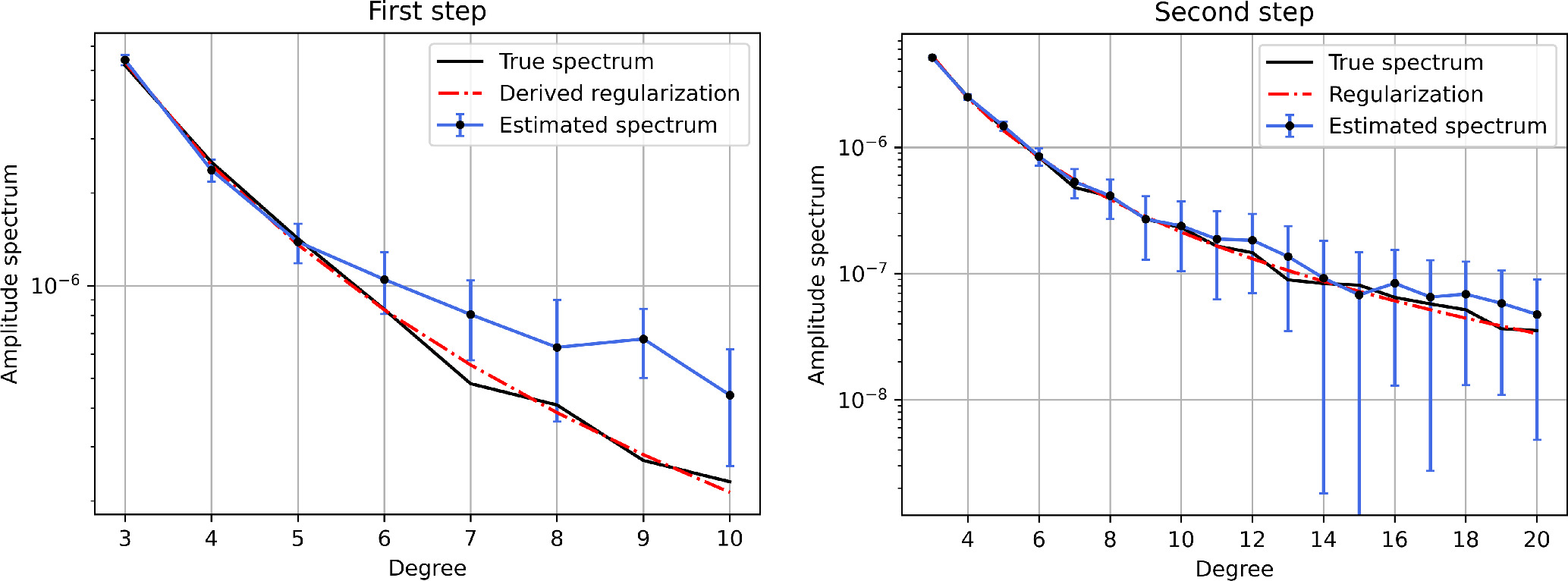
Figure 3. Outcome of the two-step solution of the gravity field. In the first step, no a priori regularization is used in the OD filter, leading to a poor solution for high degrees, mainly because of the uneven spatial coverage. The first-step solution is used to derive a regularization rule based only on the very first degrees. This data-based regularization is used as a priori in the second step. The vertical bars represent the rms uncertainty on the amplitude spectrum (Equation (7)).
Download figure:
Standard image High-resolution imageBy incorporating this regularization approach into the second OD fit, we can obtain a reliable solution for higher degrees as well. We emphasize the significance of this two-step procedure, as it enables obtaining a high-quality gravity solution without relying on any prior knowledge of the body's gravity field (except the assumption of a single power-law slope).
Using the gravity field spectrum as an observable quantity in the Bayesian inversion process requires defining the associated uncertainty, in the form of a covariance matrix.
Typically, in planetary gravity studies, the uncertainty spectrum presented alongside the amplitude spectrum is the rms value (per degree) of the retrieved uncertainty on the spherical harmonics expansion coefficients:

Although  provides useful information for determining the maximum resolution of the gravity field (or the degree strength; e.g., Konopliv et al. 1999), it does not represent the uncertainty of the power spectrum amplitude Al
. That is, it is representative of the typical error of a single coefficient at that degree (Clm
or Slm
), and it is not related to the knowledge of the total power at degree l, Al
. Standard uncertainty quantification methods can be used to derive the true uncertainty
provides useful information for determining the maximum resolution of the gravity field (or the degree strength; e.g., Konopliv et al. 1999), it does not represent the uncertainty of the power spectrum amplitude Al
. That is, it is representative of the typical error of a single coefficient at that degree (Clm
or Slm
), and it is not related to the knowledge of the total power at degree l, Al
. Standard uncertainty quantification methods can be used to derive the true uncertainty  . Two equivalent methods can be used: the linear propagation method and the clone method.
The gravity OD estimation process yields the spherical harmonics coefficients of the gravity potential and the corresponding variance–covariance matrix P .
The well-known linear propagation method is defined as

where  is defined as

with x = [C20, C21,...,Clm , S21, S22, Slm ].
An alternative method consists in generating a large number of clones (N), where each clone represents a realization of the gravity field coefficients drawn from a normal distribution with an expected value equal to the estimated coefficients and covariance matrix P , from which the uncertainty of the spectrum can be computed. The uncertainty on the spectrum is then obtained as the standard deviation (per degree) of these N spectra.
Figure 4 compares the different uncertainty quantification approaches for a simulated gravity field recovery. See Appendix A for a similar comparison applied to the lunar gravity field measured by GRAIL (Goossens et al. 2020).
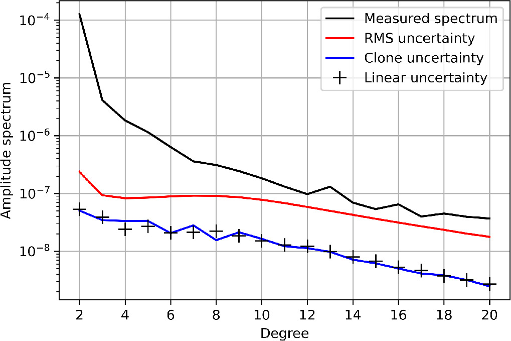
Figure 4. Comparison of different uncertainty quantification methods for the amplitude spectrum. The red line shows the conventional rms uncertainty of the measured spectrum (black line), while the blue line and black plus signs show the outcome of the clone method and the linear propagation method, respectively.
Download figure:
Standard image High-resolution imageThe clone method offers a convenient way to derive not only the uncertainty of the spectrum but also the associated variance–covariance matrix
P
A
. By generating a large set of clones, it becomes straightforward to compute the covariance between all the samples, resulting in the variance–covariance matrix. As elaborated in the subsequent section, both  and
P
A
are necessary inputs for the definition of the Bayesian likelihood.
and
P
A
are necessary inputs for the definition of the Bayesian likelihood.
We can observe that the amplitude spectrum uncertainty is consistently lower than the rms uncertainty spectrum. A substantial difference between the two quantities can be expected, as they convey different information. While the latter, as stated before, relates to the resolution of the field (i.e., the capacity of measuring gravity locally and thus of resolving single coefficients), the former gauges the capability of measuring the global power of the field. Even if the single-coefficient estimate is not accurate owing to aliasing from nonuniform coverage, the spacecraft is still highly sensitive to the averaged strength (or power) of the gravity field driving its motion.
2.3. Bayesian Inversion
Given the well-established understanding of the Markov Chain Monte Carlo (MCMC) theory, which is extensively discussed in the literature (e.g., Robert & Casella 2004; Sharma 2017), we focus our discussion on notable specifics of our method. To mitigate scaling issues caused by the broad range of magnitudes in the parameter space, we adopt the affine-invariant ensemble sampler provided by the Python library emcee (Foreman-Mackey et al. 2013; Goodman & Weare 2010). By employing this approach, we sample the parameter space with N independent chains that can be run in parallel, reducing the computational burden. To confine the sampling to a defined parameter space region, we impose rigid bounds within the likelihood function. While MCMC processes allow for various weighting schemes across different parameter space regions, we opt for uniform priors on all parameters and reject samples that fall outside these prior bounds. In addition to the sampling strategy, the fundamental component of a Bayesian inversion is the likelihood function, which governs the acceptance or rejection of samples and influences the convergence of the method. In our study, we utilize a multivariate normal distribution:

where k is the dimension of the problem (the number of observable quantities), Σ is the variance–covariance matrix of the observations,  is the determinant of Σ, and
  is the residuals vector, i.e., the vector containing the difference between the observed and computed observations. The computed observations are obtained from the forward model, while the observed ones are the result of the OD problem solution.
In the case presented here, the set of observations include the mass of the body, the moment of inertia factor (MOIF), and the gravity amplitude spectrum. We build the covariance matrix as a block matrix:

where  and
and  are the variances of the observed mass and MOIF, respectively, and Σs
is the variance–covariance matrix of the gravity spectrum of dimensions
are the variances of the observed mass and MOIF, respectively, and Σs
is the variance–covariance matrix of the gravity spectrum of dimensions  .
.
Since the gravity amplitude spectrum spans several orders of magnitude, to avoid numerical errors that may lead to overweighting of the lowest degrees, we use log(A) as an observable instead of the spectrum A. The associated covariance matrix Σs , then, is computed applying the clone method (Section 2.2) to the quantity log(A).
3. The Europa Case
3.1. The Europa Clipper Gravity Science Investigation
NASA's flagship mission Europa Clipper is scheduled to launch in 2024 October and is expected to arrive in the Jupiter system in 2030. The mission is designed for conducting an extensive mapping of Europa via a series of close encounters (flybys). The gravity/radio science (G/RS) investigation is one of the 10 investigations of Europa Clipper. It will make use of the onboard telecommunication subsystem to establish a two-way Doppler link with the Earth ground stations. In this work we simulate the G/RS investigation during the nominal mission phase, consisting of 49 flybys of Europa. We use the baseline trajectory 5 of the nominal science phase, together with a detailed model of the solar and Jupiter system ephemerides. We integrate the trajectory of the probe and produce synthetic observables based on the spacecraft and ground station antenna scheduling. This task holds significant importance for the Europa Clipper investigation, as the flyby geometry, together with the pointing requirements on the spacecraft, constrains the onboard antenna viewing geometry.
The Doppler link must be established using different assets: the high gain antenna (HGA), the fanbeam (FBA) antennas, and the low gain antennas (LGA). FBA and LGA have a lower gain with respect to the HGA, thus reducing the amount of received power at the ground station, but the HGA is not available for tracking close to Europa owing to pointing constraints. As a result, the capability of establishing a successful Doppler link, as well as its resulting noise level, depends on a complex combination of factors involving the flyby geometry, the flyby epoch, and the spacecraft science operation planning. In this work we adhere to the latest assumptions regarding the performance of the tracking system (Mazarico et al. 2023), which assume a noise threshold, for a successful Doppler link, of 4 dB-Hz.
Using the NASA-JPL software library MONTE (Evans et al. 2018), we integrate the trajectory, considering the point-mass gravitational attraction of all main solar system and Jupiter system bodies, the nonspherical contribution of Jupiter's gravity field, and Europa's gravity field (see next section). We account also for the solar radiation pressure acting on the probe, which is modeled as a cannonball. For each Europa interior model case and thus assumed gravity field, we integrate the trajectory of the probe over the 4 hr flyby periods centered on each closest approach, simulate the tracking data, compute the partial derivatives of the observables with respect to the solved-for parameters, and run a full OD solution, iterating the process until convergence. We solve the OD problem using a multi-arc approach (see, e.g., Cascioli et al. 2021; Durante et al. 2020 for further details). The full list of parameters solved for in the OD filter includes the state of the probe (position and velocity with respect to the Jupiter system barycenter), a solar radiation pressure scale factor per flyby, Europa's body fixed frame spin axis orientation and spin rate, the libration angular amplitude (at the orbital frequency), Europa's GM, the spherical harmonics coefficients of Europa's gravity field up to degree and order 20 (in the second inversion; see Section 2.2), and the tidal Love number k2.
One of the objectives of the G/RS investigation is the measurement of Europa's MOIF ( , with C the polar moment of inertia and M and R the mass and radius of the body, respectively). The measurement accuracy on the MOIF depends on whether Europa satisfies hydrostatic equilibrium (Mazarico et al. 2023). While the icy shell is believed to meet the equilibrium condition because of its low rigidity, less certain predictions can be made about the silicate interior. Previous analyses of Galileo encounters of Europa implicitly assumed hydrostaticity (Anderson et al. 1998; Jacobson et al. 2000), while recent efforts have obtained solutions of Europa's gravity field relaxing the assumption (Gomez Casajus et al. 2021). The predominantly equatorial coverage of the Galileo encounters prevents a reliable estimate of both J2 and C22, resulting in substantial uncertainties, and precluding concluding whether Europa is in hydrostatic equilibrium or deviates from it. This consideration impacts the various methods employed to estimate the MOIF.
If measurements from Europa Clipper confirm that the body is in hydrostatic equilibrium, the Radau–Darwin equation, which relates J2, C22, and MOIF, can be directly used, yielding a predicted uncertainty on the MOIF of approximately 1.5 × 10⁻⁴. However, if the Radau–Darwin relationship cannot be used, alternative methods must be employed, leading to a higher uncertainty of the order of 2.3 × 10⁻³ (see Mazarico et al. 2023 and references therein for a comprehensive discussion on this topic).
As discussed in Section 2.2, the second observable quantity employed in the Bayesian inversion is the mass of the body. It serves the purpose of maintaining internal consistency within the inversion process. The uncertainty associated with the mass is derived from the estimated uncertainty of GM, multiplied by a factor of 1000. We use an uncertainty value of 8.8 × 10¹⁸ kg, which corresponds to approximately 0.01% of Europa's mass.
3.2. Europa Interior
We establish a reference case for Europa by adopting values for key model quantities that align with those published in previous studies (Pauer et al. 2010; Koh et al. 2022). Table 1 reports the values used as a baseline. It can be argued that the chosen value of the maximum silicate layer topography (2 km) is relatively small, if compared to other differentiated silicate worlds in the solar system (e.g., Wieczorek 2015; Ermakov et al. 2018). However, it will be clear in the next section (and Appendix B) that this assumption constitutes a worst-case scenario for the methodology we propose in this work, as a larger topography would imply a stronger gravitational signal of the seafloor and thus a better overall sensitivity to it, resulting in a better determination.
Some authors, moreover, have predicted the possible presence of a thick (3–10 km) sedimentary layer of gypsum on the seafloor (Melwani Daswani et al. 2021). Two possible end-member models, as proposed by Koh et al. (2022), would consist of a flattening of the seafloor due to the gypsum deposits filling the topography, or alternatively a uniform blanket that would uniformly increase the seafloor topography. While the second end-member does not have any significant effect on the gravity signal of the seafloor (as shown by Koh et al. 2022), the first end-member can substantially change its amplitude. Although not explicitly introduced here, we argue that this end-member case can be equivalently modeled by either a modification of the density contrast between the silicate crust and the ocean or a reduction of the topographic profile (as a consequence of Equations (3a) and (3b)). Among the end-member models we tested in this work (table in Figure 5), we have considered ample variations in the topographic profiles, thus implicitly accounting for the possible presence of a sedimentary deposit on the base of the ocean.
The gravity model based on parameters from Table 1 is shown in Figure 6. The difference between the gravity fields of the silicate ocean floor and the icy shell is particularly evident in the scale of the associated gravity anomalies.
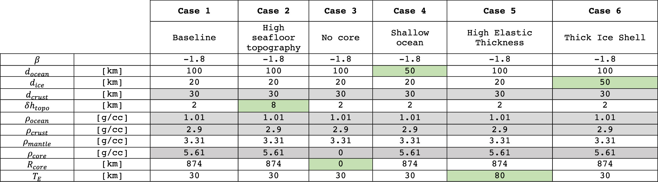
Figure 5. Europa's interior structure end-members used in this work. Gray cells denote parameters that are not solved for but perturbed for robustness. Green cells denote parameters that are different with respect to the "Reference" case.
Download figure:
Standard image High-resolution image
Figure 6. Gravity anomalies associated with the reference Europa interior structure, expanded up to degree and order 30.
Download figure:
Standard image High-resolution imageThe icy shell's low rigidity leads to isostatic compensation at the longest wavelengths, resulting in the suppression of large-scale anomalies and the prominence of smaller scales. Conversely, the higher rigidity of the seafloor enables the persistence of significant power in longer spatial scales. This fundamental mechanism allows us to effectively distinguish and separate the contributions of the two.
The morphology and amplitude of the resulting gravity spectrum are highly dependent on the choice of the physical parameters defining the body's interior. Figure 7 shows the effect of varying the ocean depth. Variations in the ocean depth result in strong variations in the amplitude and shape of the gravity spectrum and variations in the MOIF larger than the measurement uncertainty.

Figure 7. Sensitivity of the gravity spectrum (left) and MOIF (right) to variations of the ocean depth. The shaded areas in the right panel represent the predicted uncertainty in the MOIF retrieval in the case of hydrostatic equilibrium (yellow area) and nonhydrostatic equilibrium (blue area).
Download figure:
Standard image High-resolution imageTo ensure a comprehensive exploration of the sensitivity of the Bayesian inversion process, we recognize the need to consider multiple cases rather than relying on a single interior structure scenario. Figure 7 serves as an illustrative example, demonstrating that the amplitude of the gravity spectrum depends on the interior structure configuration. This variation implies differing degrees of sensitivity for the spacecraft measurements. Specifically, a deep ocean scenario results in a reduced amplitude and lower sensitivity to seafloor variations, while a shallow ocean scenario gives greater sensitivity, potentially leading to a more robust determination of the ocean depth and seafloor parameters. Consequently, we conducted an extensive examination of the parameter space, encompassing a wide range of cases that represent the extreme ends of the spectrum. We explored the parameter space, varying the main parameters of the model (see Appendix B for the full set of figures). We were thus able to determine the subset of parameters whose plausible variations have a limited impact on the spectrum and moment of inertia, allowing us, then, to fix them and not solve for them. From the other, more important parameters, we defined six different interior structure scenarios. The table in Figure 5 details these six cases we will explore in the following.
As the figure shows, we chose to fix dcrust, ρocean,  , and ρcrust because of the reduced sensitivity of the observables to these parameters. By reducing the number of solved-for parameters, we mitigate correlations among them and minimize the dimensionality of the parameter space, thereby improving computational efficiency. However, to test the solution's robustness against potential biases resulting from fixed parameter assumptions, we define subcases where these parameters are still held fixed during inversion but perturbed off the actual, correct value (Table 2). The amount of perturbation is determined by assessing the parameter space (Appendix B) and identifying the variations corresponding to a 3σ offset from the computed average MOIF value (with 1σ representing the predicted uncertainty in the hydrostatic case). This approach ensures a thorough evaluation of the solution's sensitivity to variations in these parameters.
Table 2. Definition of Subcases
| Model Value | 3σ Distance | Subcase a | Subcase b | Subcase c | |
|---|---|---|---|---|---|
| dcrust (km) | 30 | 20 | + | ⋯ | ⋯ |
| ρocean (g cc–1) | 1.01 | 0.03 | + | + | + |
| ρcrust (g cc–1) | 2.9 | 0.12 | + | ⋯ | + |
 (g cc–1) (g cc–1) | 5.61 | 0.3 | ⋯ | + | ⋯ |
Note. Plus and minus signs indicate that the 3σ distance is added or subtracted to the model value. The 3σ distance is defined as the parameter value corresponding to a distance equivalent to three times the predicted formal uncertainty on the MOIF in the hydrostatic case.
Download table as: ASCIITypeset image
4. Results and Discussion
The full process described in the previous sections, including the generation of the truth model, the OD simulation, and the Bayesian inversion, is conducted for a total of 24 cases: the 6 main cases shown in Figure 5, each with 3 additional perturbed subcases. In order to ensure the robustness of our conclusions, the OD simulations are performed in a full recovery fashion. This involves generating synthetic observables from the correct Europa gravity model, while using a different starting value in the OD estimation process. As a result, the OD filter is iterated, adjusting all the solved-for parameters until reaching suitable convergence. In the Bayesian process, we solve for and monitor the estimation outcome of eight parameters ( , and the hydrosphere thickness dH
= docean + dice). In all the analyzed cases, alongside the separate estimates of docean and dice, we compute and assess the estimate of the total depth of the hydrosphere, dH
, for a grand total of 192 posterior marginal distributions.
, and the hydrosphere thickness dH
= docean + dice). In all the analyzed cases, alongside the separate estimates of docean and dice, we compute and assess the estimate of the total depth of the hydrosphere, dH
, for a grand total of 192 posterior marginal distributions.
To simplify the interpretation of the results, we introduce two compact metrics similar to those proposed by Biersteker et al. (2023), with slight adaptations to suit the specific problem at hand. These metrics allow for a more straightforward analysis of the inversion outcomes. Here we provide a brief overview of their definition.
We are interested in two main factors: the accuracy and the precision of the estimate. The first metric, M1, measures the accuracy of the estimate, i.e., how close the estimate is to the true value given the estimation error. The second metric, M2, measures the precision of the estimate, i.e., how informative the retrieved estimate is.
The first metric, M1, assesses the accuracy of the estimate by measuring how close the estimated value is to the true value. We classify the M1 outcome as Pass if the true value falls within the 68.27th percentile highest-density interval (HDI) of the estimated posterior marginal distribution. If the true value is within the 99.7th percentile HDI, we consider the outcome as Marginal. Otherwise, if the true value lies outside both intervals, we consider it a Fail. These HDI intervals correspond to the 1σ and 3σ intervals of a normal distribution. 6
The second metric, M2, evaluates the informativeness of the retrieved posterior distribution. We define a goal for each estimated parameter, represented by the desired uncertainty bound up of the parameter p. The goal of the experiment is to estimate the parameter with a precision equal to or better than ptrue ± up . The M2 outcome is classified as Pass if ptrue ± up contains 68.27% of the probability mass, Marginal if it contains 50% of the probability mass, and Fail otherwise. Table 3 reports the selected values for up .
Table 3. Values of up Used for the Computation of M2 and Uniform Priors Used for Parameter Space Sampling
| Parameter | up | Uniform Prior |
|---|---|---|
| β | 0.3 | [1, 3] |
| docean | 30% | [0, 200] km |
| dice | 30% | [0, 80] km |
| δ htopo | 1.5 km | [0, 10] km |
| ρmantle | 0.3 g cc−1 | [2.9, 5] g cc−1 |
| Rcore | 150 km | [0, 1000] km |
| TE | 15 km | [0, 100] km |
Download table as: ASCIITypeset image
Europa Clipper has an established science objective of achieving a 50% uncertainty bound (up ) for docean and dice. However, in certain cases we examined, a ±50% range would encompass a significant portion of the uniform prior distribution we defined. To address this, we adopt a more stringent value of 30% for these parameters. For the remaining parameters, we select values corresponding to 15% of the width of the prior distribution, as summarized in Table 3. These chosen values aim to ensure a reasonable level of precision in estimating the parameters during the inversion process. For the hydrosphere depth, we set a value of 30% in analogy with docean and dice.
In the following, we compare the quality of Europa's interior structure inversion using the method proposed in this work, referred to as MMS (mass, MOIF, spectrum), with the results obtained using only mass and MOIF, referred to as MM. The results of the two metrics are presented in the tables in Figures 8 and 9, along with numerical information on the quality of the solution for both the hydrostatic and nonhydrostatic cases.
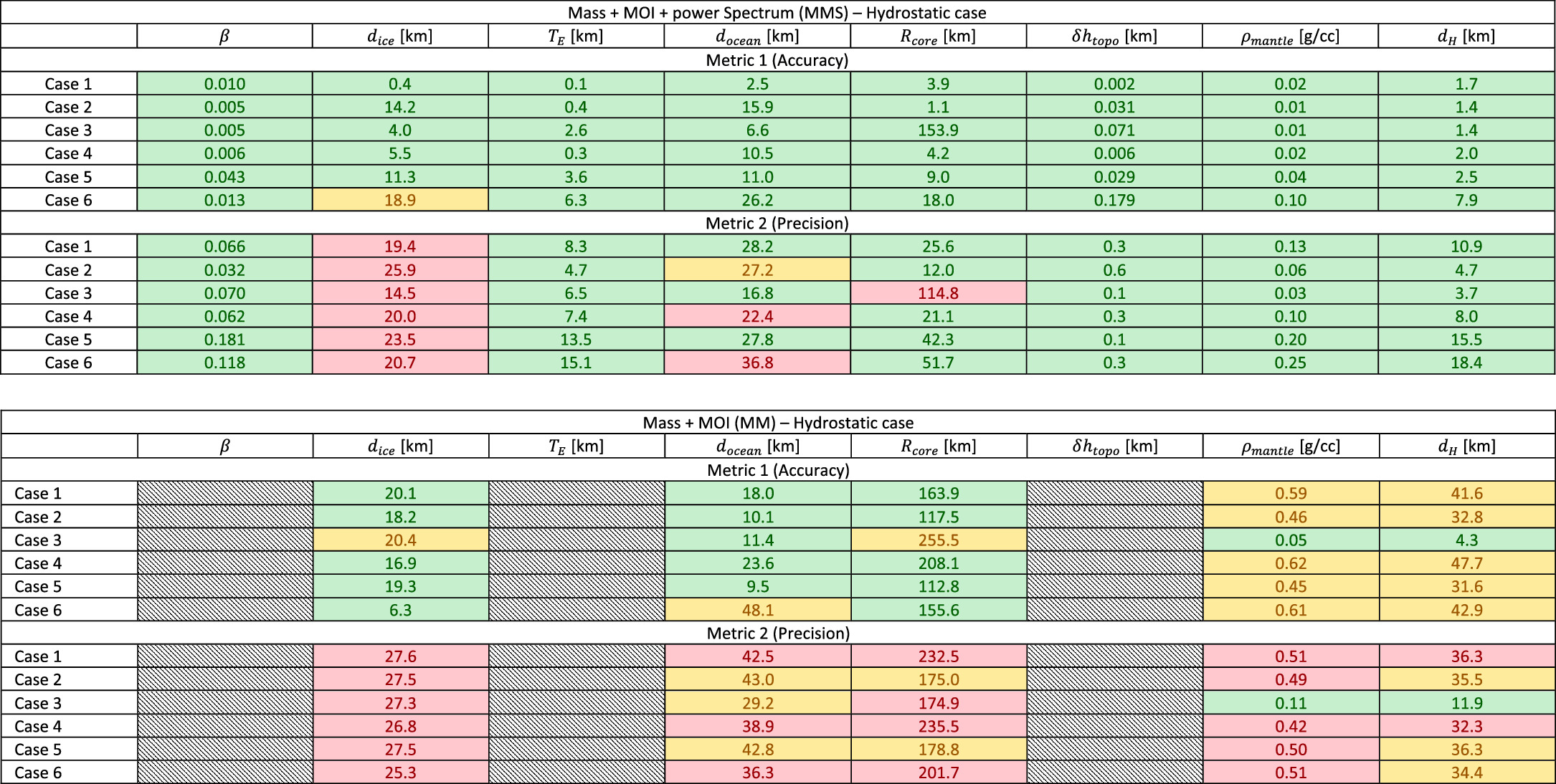
Figure 8. Bayesian inversion results for the hydrostatic case in the MMS and MM scenarios. The tables report the outcome of the two metrics in colors (green = Pass, yellow = Marginal, red = Fail). The numerical values for Metric 1 report the estimation error (as defined in the text, true value – estimated value), and the Metric 2 numerical values report the width of the 68.7% HDI interval, corresponding to the width of ±1σ for a normal distribution).
Download figure:
Standard image High-resolution image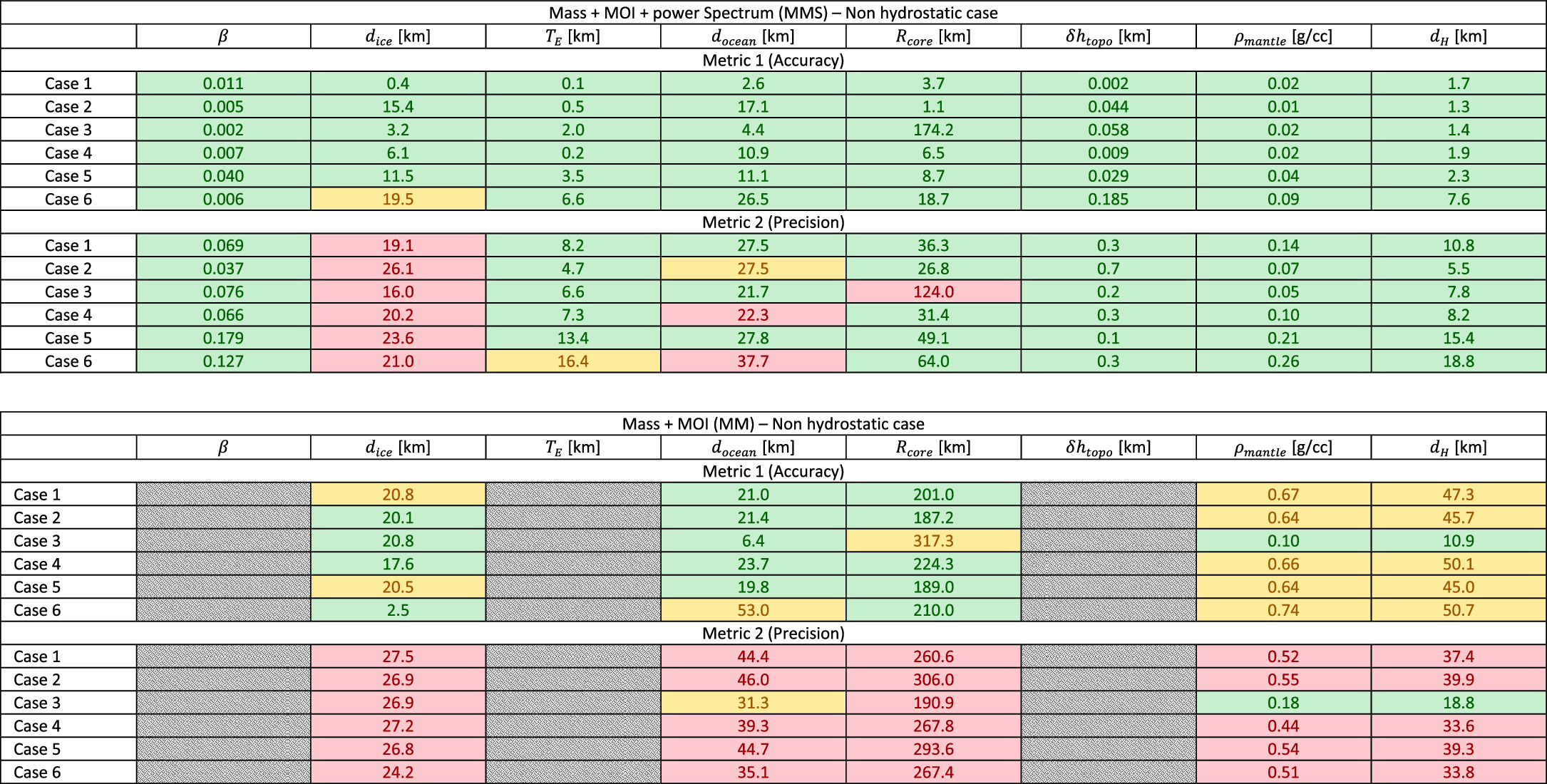
Figure 9. Bayesian inversion results for the nonhydrostatic case in the MMS and MM scenarios. The tables report the outcome of the two metrics in colors (green = Pass, yellow = Marginal, red = Fail). The numerical values for Metric 1 report the estimation error (as defined in the text, true value – estimated value), and the Metric 2 numerical values report the width of the 68.7% HDI interval, corresponding to the width of ±1σ for a normal distribution).
Download figure:
Standard image High-resolution imageTogether with the metric result (Pass/Marginal/Fail), we report the numerical values of the estimation error (the difference between the true value and the median of the posterior distribution) and the width of the 68.27% HDI interval, corresponding to the ±1σ interval for a normal distribution.
The difference between the metrics of the two solutions (MMS and MM) is significant. While the MMS solution mostly passes all the metrics, the MM solution fails to provide a robust inversion of the interior of Europa.
The MMS solution allows us to consistently and reliably determine almost all the parameters of interest except dice, with a few notable exceptions. Although the reliability of the estimate of the ocean depth depends on the specific end-member case, the estimation of the hydrosphere depth is robust, leading to an uncertainty ranging between 4 and 20 km satisfying, with margin, the Europa Clipper science requirements. The nonreliability of the estimate of dice mainly results from the limited range of sensitivity of Europa Clipper, given that only the low degrees of the gravity field are measured. As shown in Figure 2, the gravity field of a body like Europa starts to be dominated by the ice shell at degrees higher than l ∼ 35, whereas the Europa Clipper sensitivity to the gravity degree spectrum Al is capped at l < 20.
The ocean floor properties, such as the elastic thickness TE
, the maximum topography δ
htopo, and the topography logarithmic slope β, are consistently well determined, as are the core density and the deep interior properties (Rcore and ρmantle), except for the core radius in the no-core case (Case 3). In this specific scenario, the posterior distribution exhibits a significant spread, leading to a Fail in M2 (although the probability mass is 48%, just below the Marginal requirement of 50%). It is important to underline, however, that the overall estimate ( km) is compatible at the 3σ level with the absence of a core.
Additionally, the use of the gravity spectrum as an observable leads to a general reduction of the interior model parameter uncertainties. Intuitively, this is because additional information is used in the inversion, but also because it provides new information, allowing us to strongly reduce some of the correlations between the solved-for parameters.
As explained above, besides the nominal cases, where the fixed parameter values are set to their true value (dcrust,  ), we run three subcases for each nominal case, in which we set these parameters to values different from the truth. This approach allows us to test the robustness of the solution to biases and assess whether incorrect assumptions can lead to misleading estimates. For all the main cases we tested, the subcase results align well with the main case, highlighting the robustness of the solution (for the complete set of results see Appendix C).
Figures 10 and 11 show the estimated posterior distributions for Case 4. Figure 10 directly compares the posterior distributions of the parameters common to both MM and MMS inversions, while Figure 11 shows the estimated posterior distributions of the parameters that are solved for only in the MMS case. The combined inversion results in an overall improvement in the statistical properties of the posterior distributions, which become more concentrated around the true values. Notably, the utilization of the gravity field spectrum as an additional observable enhances the observability of the system and significantly reduces certain correlations in the parameter space, such as those between dice, Rcore, and ρmantle.

Figure 10. Common parameters: estimated posterior distributions in the Case 6 scenario; comparison of the posterior distributions of the Bayesian inversion showing only the parameters to which both methods are sensitive. The brown quantities are relative to the MOI-only case, while the blue quantities are relative to the combination of MOI, Mass, and gravity spectrum. The solid black lines show the true value of the parameters used as input to the whole process.
Download figure:
Standard image High-resolution image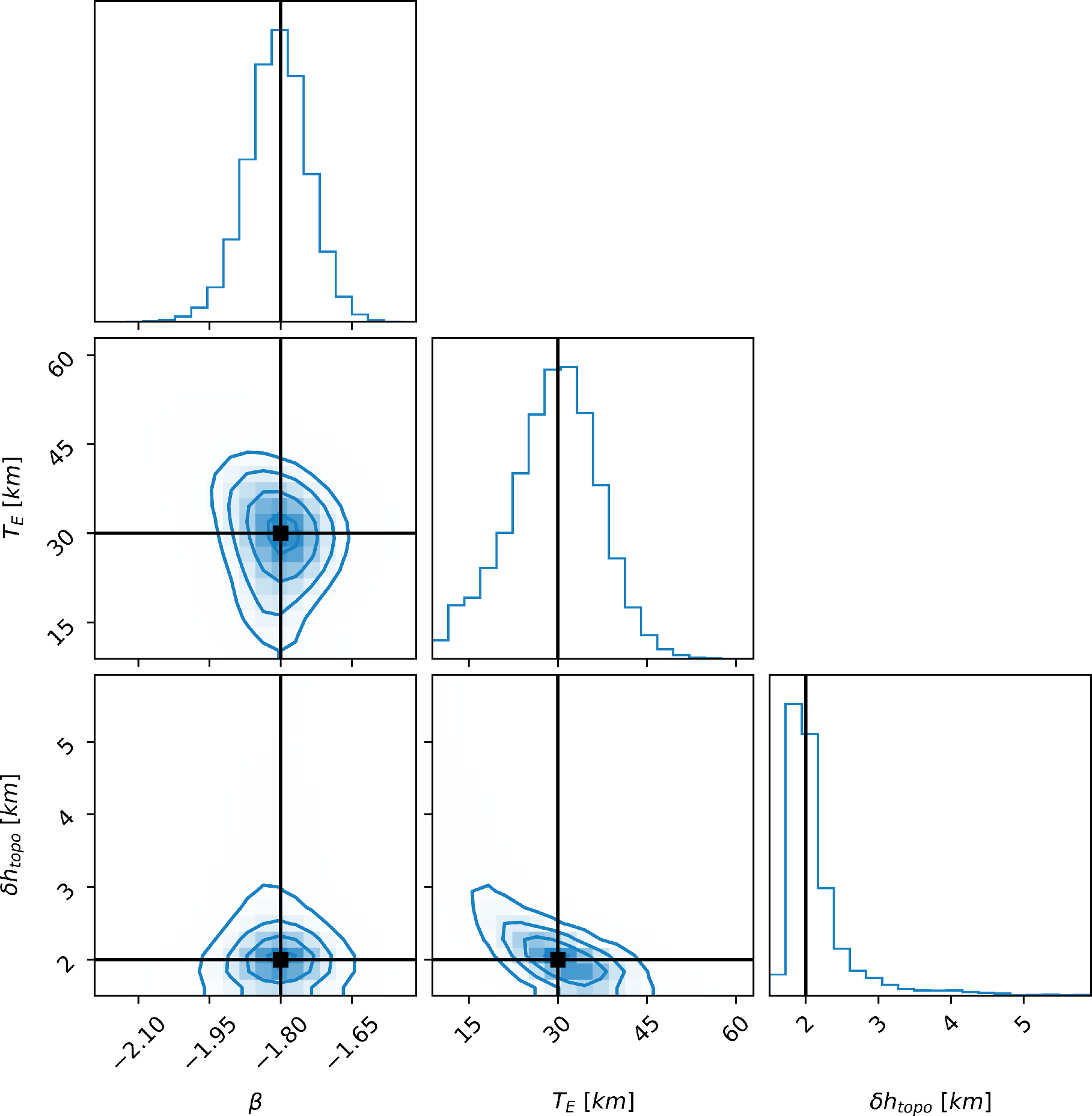
Figure 11. Parameters specific to the MMS method: estimated posterior distributions in the Case 6 scenario; comparison of the posterior distributions of the Bayesian inversion showing the parameters to which only the MMS method is sensitive. The solid black lines show the true value of the parameters used as input to the whole process.
Download figure:
Standard image High-resolution imageIt is worth noting that in this specific case both dice and docean fail the second metric owing to the wide spread of their posterior distributions. However, they exhibit substantial accuracy, as indicated by the Pass outcome of M1. Here the probability mass contained in the docean ± 30% and dice ± 30% intervals is 47% and 23%, respectively.
As expected, β has a nonnegligible correlation with some of the other solved-for parameters. Specifically, it has a 50%–55% correlation with Rcore, ρmantle, and dH , and 15% or lower with the rest of the parameter space. Although significant, this correlation pattern does not hinder the quality of the solution, as testified by the outcome of the perturbed subcases, which do not show signs of biasing.
Although not affecting the general picture, the hydrostatic assumption influences the parameter retrieval uncertainty as expected, with higher uncertainties in the nonhydrostatic case. Interestingly, however, this uncertainty increase effect is much stronger for the MM solution, whereas it is more subdued in the MMS scenario. This is mainly reflected in the Metric 2 outcome, which presents more Fail occurrences compared to the hydrostatic case, while the MMS metrics are not affected by the hydrostatic assumption. This is particularly interesting for the uncertainty associated with dH , which remains substantially identical in the two cases.
We can draw the general conclusion that the method proposed in this work allows us to obtain an unbiased and informative estimate of the hydrosphere depth for all the end-member cases we tested with an uncertainty lower than 20 km in all cases. Separate observability of dice and docean is not attainable with the proposed method, under the assumed measurement uncertainties; however, it is important to underline that the estimates of these parameters never fail Metric 1, meaning that the estimate is unbiased but not informative enough to the standards we have set (see Table 3). Notably, docean passes Metric 2 in some cases. This fact is particularly interesting considering that Europa Clipper will also measure the tidal response and magnetic field of the body. The tidal response (tidal potential and deformation combined) provides observability to the ice shell thickness and rigidity (Wahr et al. 2006; Mazarico et al. 2023), while the magnetic induction measurement provides sensitivity to the ocean thickness and to a lesser extent to the ice shell thickness (Biersteker et al. 2023; Petricca et al. 2023). Both these methods require some model assumptions. For example, the ice shell thickness derived from the tidal response cannot be unambiguously separated from the hypothesized ice rheology. Similarly, the modeling of the magnetic field arising from the Europa-ambient magnetospheric plasma interaction plays an important role in the estimation of the ice thickness from magnetic induction measurements. As evidenced and thoroughly discussed by Roberts et al. (2023), the strength of Europa Clipper will lie in its synergistic investigations, each providing a different view of the interior of Europa. The method we developed in this work will likely serve this very purpose: not only would it act as an independent validation for the magnetic induction response measurements, by providing a constraint on the total hydrosphere thickness and possibly on the ocean thickness in some cases, but it would also strengthen the interior structure inversions based on tidal and magnetic response with complementary and independent information. Additionally, it offers observability to important parameters related to the deep interior and seafloor topography. Our results indeed show that the deep interior-related parameters are reliably estimated: Rcore is measured within 50 km uncertainty in all cases, except Case 3 as discussed above; ρmantle is estimated within 0.25 g cc−1 uncertainty. The proposed method also provides an excellent determination of the seafloor characteristics providing estimates of TE , δ h , and β to within 5–15 km, 100–600 m, and 0.03–0.2, respectively, depending on the actual interior characteristics.
In this work, we have focused on the deep interior, due to the Europa Clipper measurement capability limited to the lowest degrees of the gravity field. Other missions investigating icy bodies will obtain higher gravity field resolutions (e.g., JUICE at Ganymede; Cappuccio et al. 2020) and will benefit from the proposed method by concurrently evaluating the characteristics of the ice shell, such as its elastic thickness and its density, and more general parameters affecting the gravity field spectrum above the measurement noise level.
5. Conclusion
In this work we have investigated the possibility of using the measured gravity field spectrum as an additional observable for the inversion of the interior structure of differentiated icy bodies. After developing the general methodology, we have applied it to the Europa case simulating the future gravity field measurements by NASA's Europa Clipper. We have thoroughly tested the proposed method by simulating six different end-member scenarios and evaluated the quality of the interior structure inversion. Our analysis shows that the proposed use of the gravity field spectrum as an observable provides significant sensitivity on key parameters of the icy body interior. Notably, we have shown that the hydrosphere (ice shell + ocean) thickness can be resolved with an uncertainty in the range of 4–20 km (depending on the specific end-member case) and that the proposed method provides, in all the tested cases, a reliable estimate of the maximum topographic range, the elastic thickness of the seafloor with uncertainty ranges of 5–15 km and 100–600 m, respectively, and the density of the silicate mantle and the radius of the silicate core estimated within 0.25 g cc−1 and 50 km, respectively. The method developed in this work has a large range of applications, as it can be easily applied to other bodies, extended to more complex interior structure models, and expanded to include additional measurements such as the tidal response or the magnetic induction. Additionally, in the case of anticipated higher gravity field resolution (e.g., JUICE at Ganymede), the proposed method can directly be employed to probe additional physical characteristics of the ice shell.
Acknowledgments
Work by G.C. was supported by NASA under award No. 80GSFC21M0002.
Appendix A: Grail Amplitude Spectrum Analysis
Here we show the Moon's gravity spectrum amplitude uncertainty computed with the different methods outlined in Section 2.2. We use the GRGM1200A Moon gravity field (Goossens et al. 2020) truncated to l = 660. We compute the uncertainty using the three distinct methodologies discussed in Section 2.2 and show the results in Figure A1. Although truncated at degree 180 for computational reasons (the covariance matrix becomes too big to fit in memory), the linear propagation method shows a good agreement with the clone method.

Figure A1. The Moon's gravity field (GRGM1200A) amplitude spectrum and associated uncertainty.
Download figure:
Standard image High-resolution imageAppendix B: Sensitivity Analysis
Starting from the reference Europa model (Table 1), we have computed the gravity field spectrum and the MOIF varying the model parameters one at a time. In the following we report a set of figures (Figures B1–B11) composed of two panels each. The left panel shows the total gravity field spectrum as a function of the specific interior parameter value, and the right panel shows the computed value of the MOIF as a function of the parameter value. For comparison, the right panel reports also the expected Europa Clipper MOIF measurement uncertainty with (yellow shaded area) and without (blue shaded area) the assumption of hydrostatic equilibrium.

Figure B1. Effect of changing β on the gravity spectrum (left) and on the MOIF (right). The shaded areas have the same meaning as Figure 7.
Download figure:
Standard image High-resolution image
Figure B2. Effect of changing dice on the gravity spectrum (left) and on the MOIF (right). The shaded areas have the same meaning as Figure 7.
Download figure:
Standard image High-resolution image
Figure B3. Effect of changing dcrust on the gravity spectrum (left) and on the MOIF (right). The shaded areas have the same meaning as Figure 7.
Download figure:
Standard image High-resolution image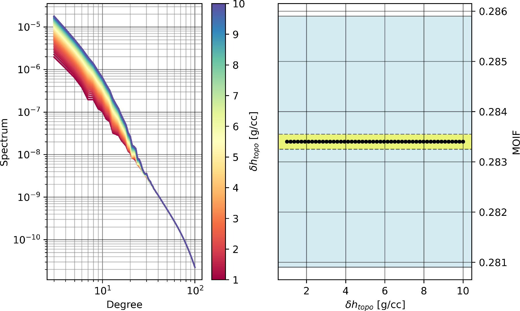
Figure B4. Effect of changing δ htopo on the gravity spectrum (left) and on the MOIF (right). The shaded areas have the same meaning as Figure 7.
Download figure:
Standard image High-resolution image
Figure B5. Effect of changing docean on the gravity spectrum (left) and on the MOIF (right). The shaded areas have the same meaning as Figure 7.
Download figure:
Standard image High-resolution image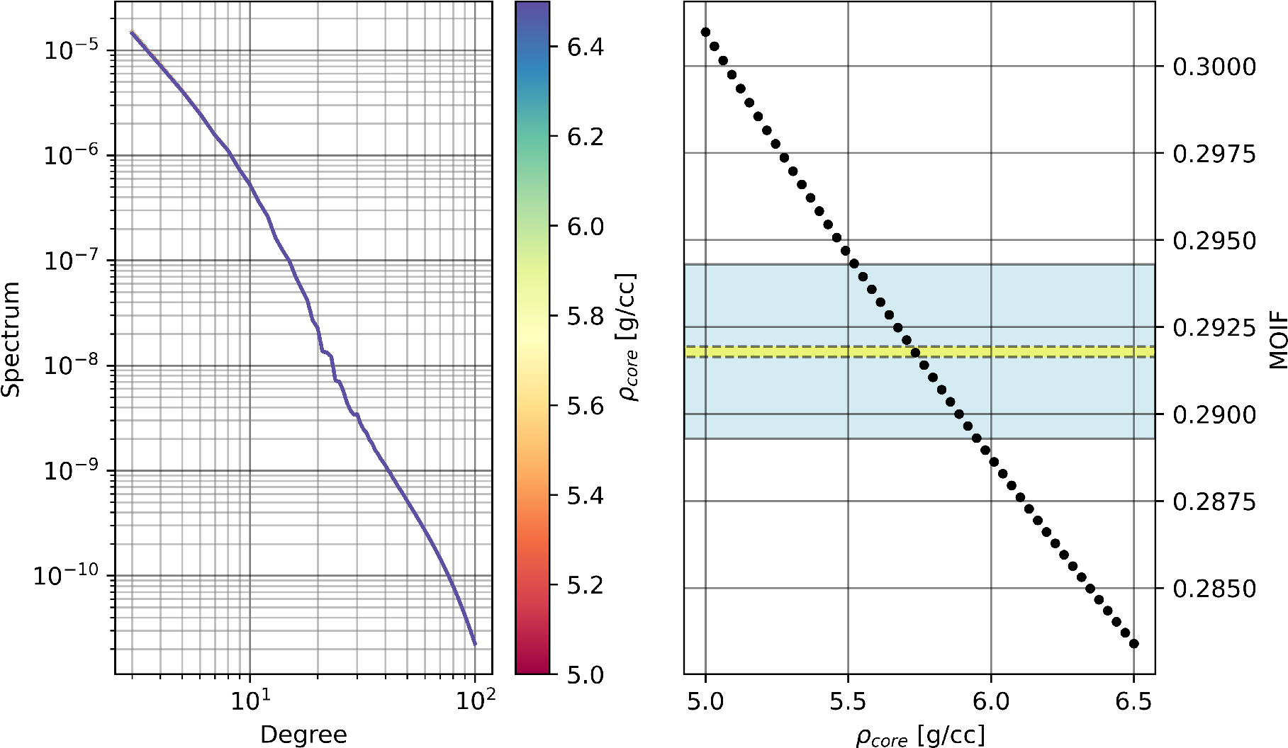
Figure B6. Effect of changing ρcore on the gravity spectrum (left) and on the MOIF (right). The shaded areas have the same meaning as Figure 7.
Download figure:
Standard image High-resolution image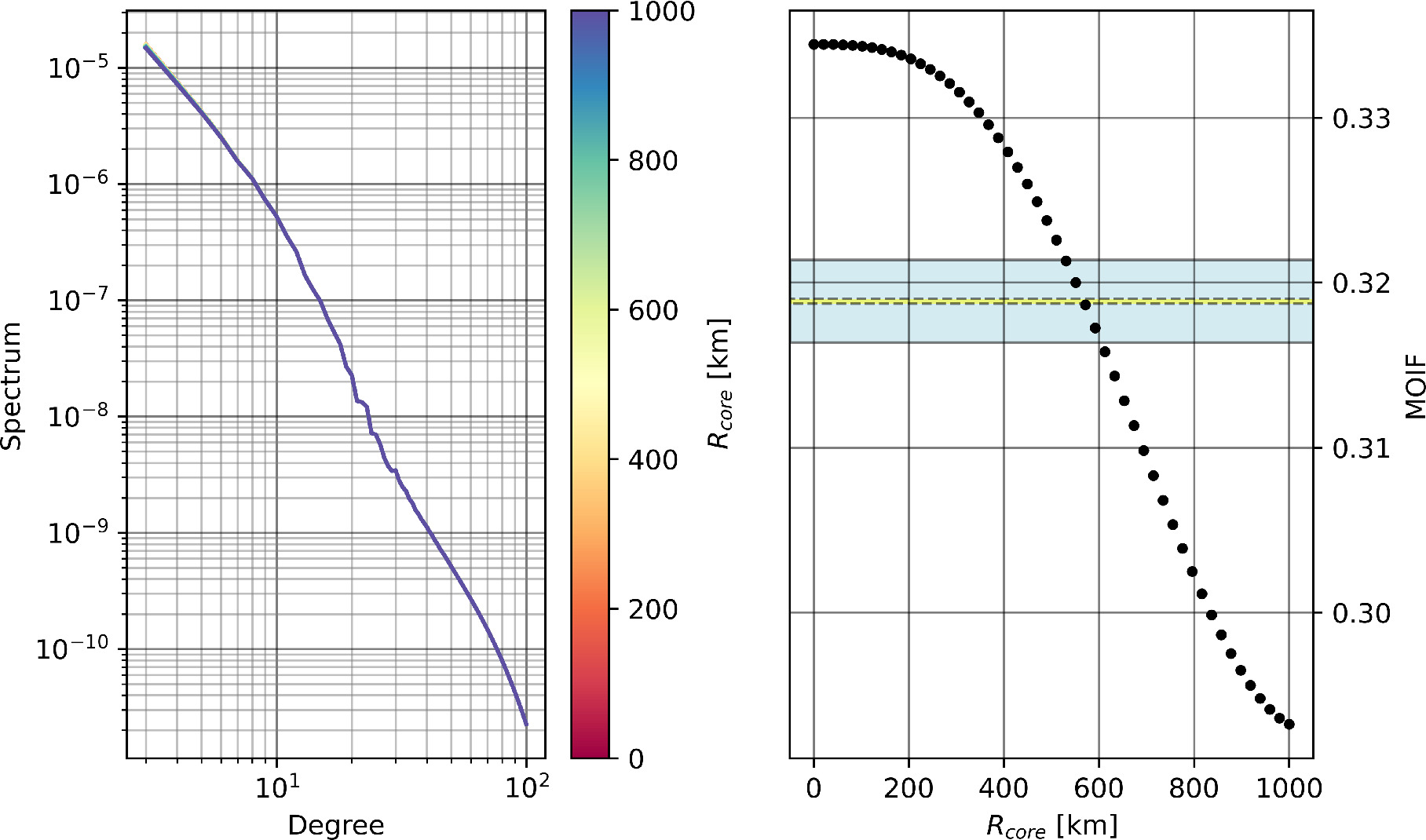
Figure B7. Effect of changing Rcore on the gravity spectrum (left) and on the MOIF (right). The shaded areas have the same meaning as Figure 7.
Download figure:
Standard image High-resolution image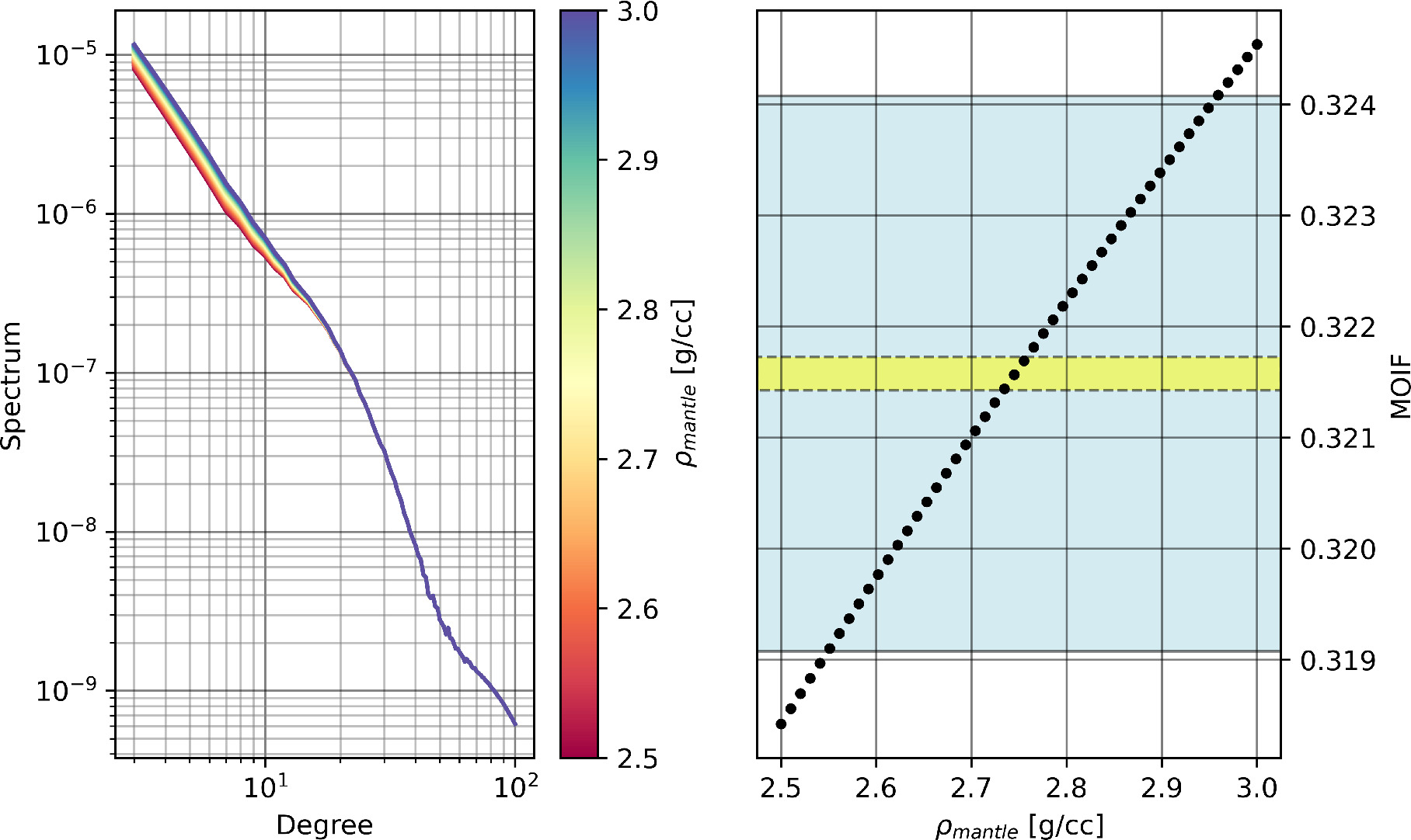
Figure B8. Effect of changing ρmantle on the gravity spectrum (left) and on the MOIF (right). The shaded areas have the same meaning as Figure 7.
Download figure:
Standard image High-resolution image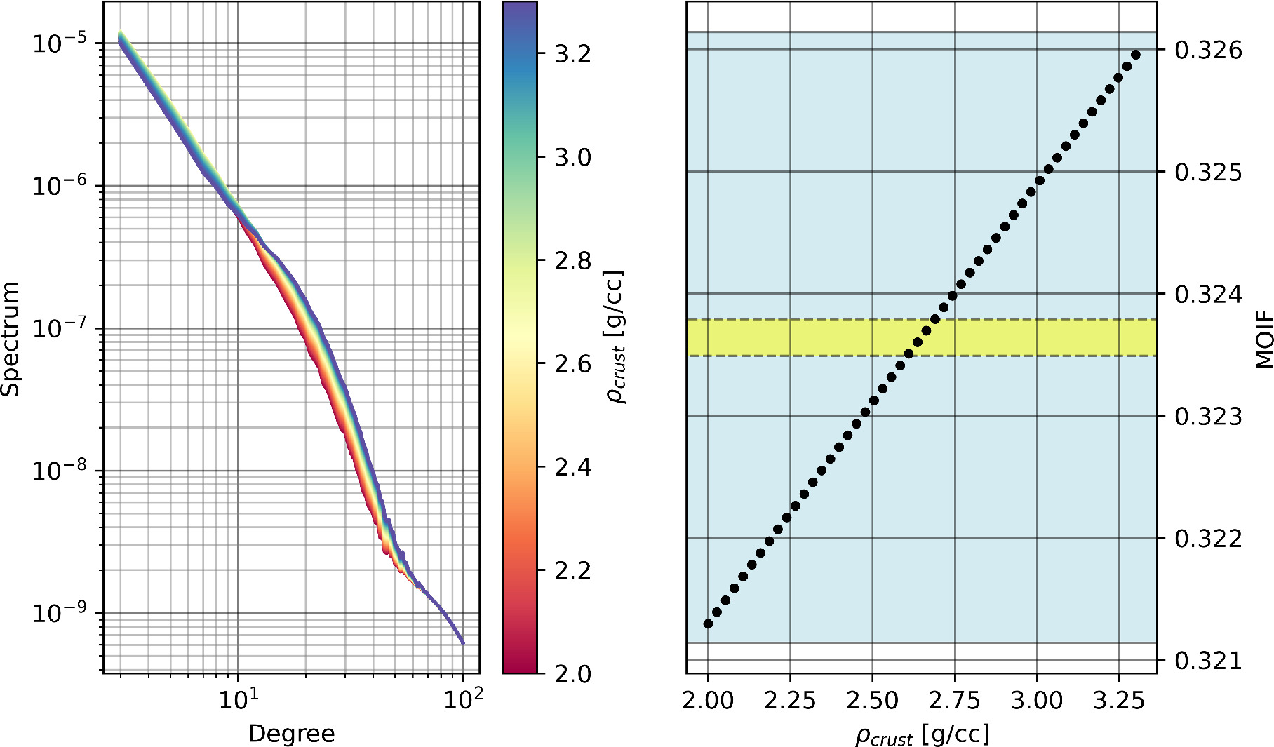
Figure B9. Effect of changing ρcrust on the gravity spectrum (left) and on the MOIF (right). The shaded areas have the same meaning as Figure 7.
Download figure:
Standard image High-resolution image
Figure B10. Effect of changing Te on the gravity spectrum (left) and on the MOIF (right). The shaded areas have the same meaning as Figure 7.
Download figure:
Standard image High-resolution image
Figure B11. Effect of changing ρwater on the gravity spectrum (left) and on the MOIF (right). The shaded areas have the same meaning as Figure 7.
Download figure:
Standard image High-resolution imageAppendix C: Full Solutions
Here we report the full set of results of our simulations. Each table (Figures C1–C4) reports the M1 and M2 values (as defined and discussed in Section 4) for all the nominal cases and the perturbed subcases. The case names are assigned according to the following nomenclature:
Case Xy, where X indicates the case number and y indicates the subcase (either nominal (n) or one of the three perturbed subcases a, b, c).

Figure C1. Full results for the MMS-Hydrostatic case. The numbers and colors follow the same definition as Figures 8 and 9.
Download figure:
Standard image High-resolution image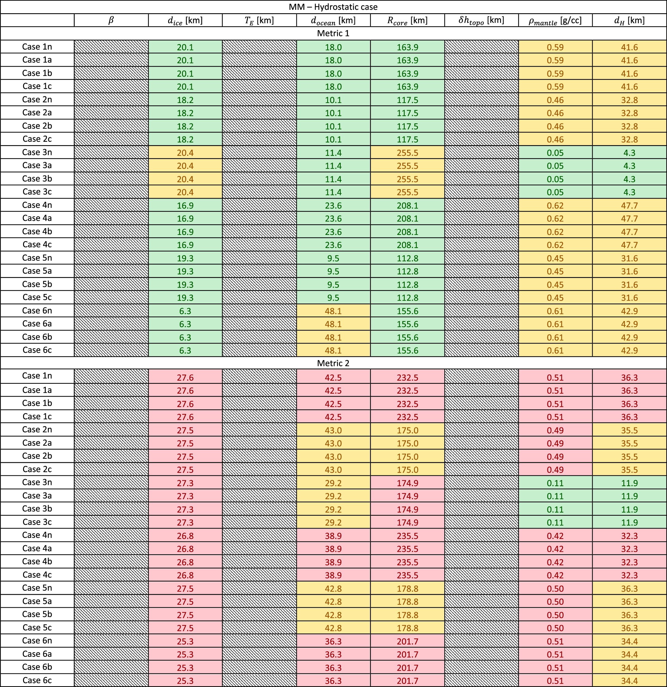
Figure C2. Full results for the MM-Hydrostatic case. The numbers and colors follow the same definition as Figures 8 and 9.
Download figure:
Standard image High-resolution image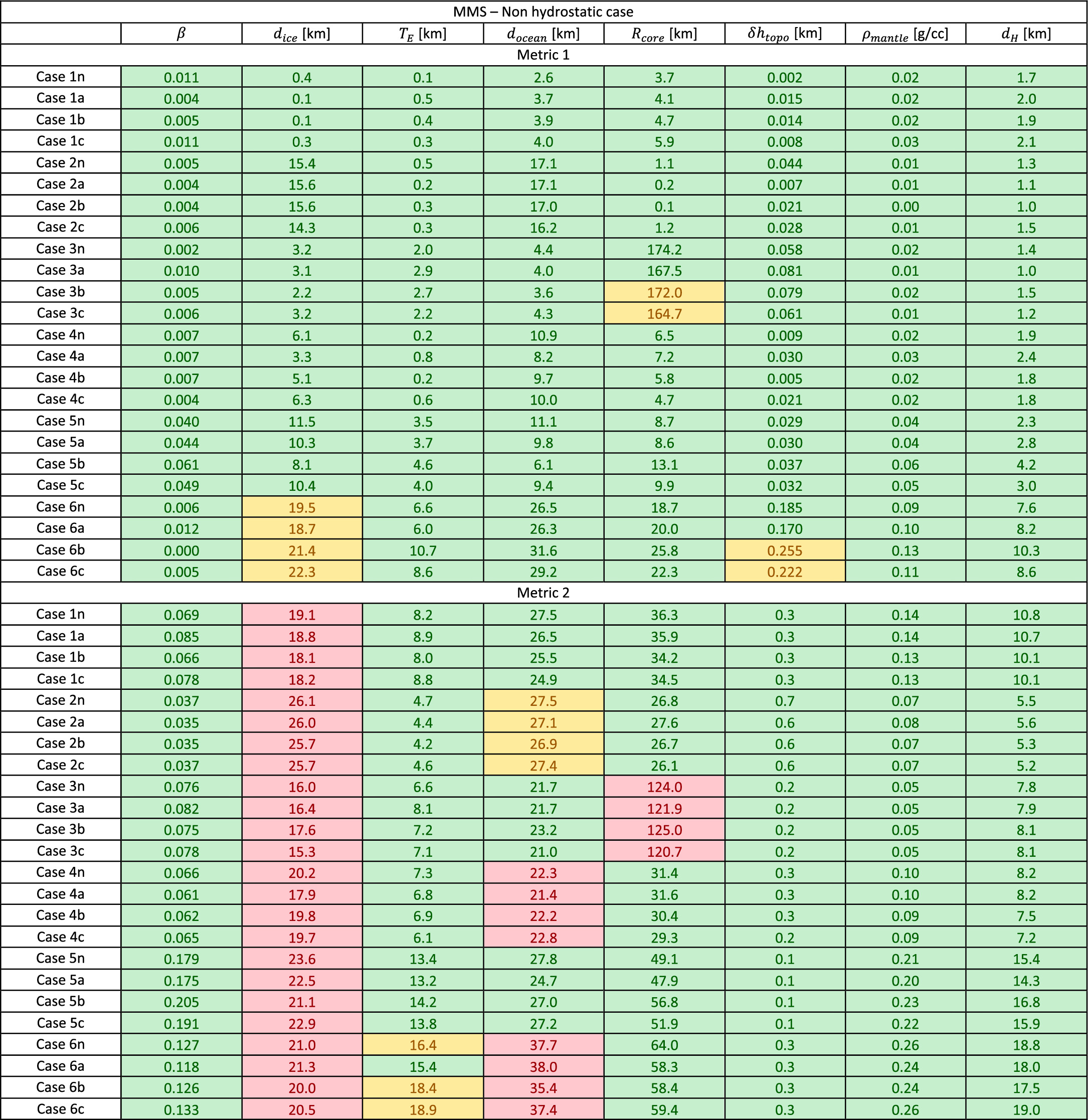
Figure C3. Full results for the MMS-Nonhydrostatic case. The numbers and colors follow the same definition as Figures 8 and 9.
Download figure:
Standard image High-resolution image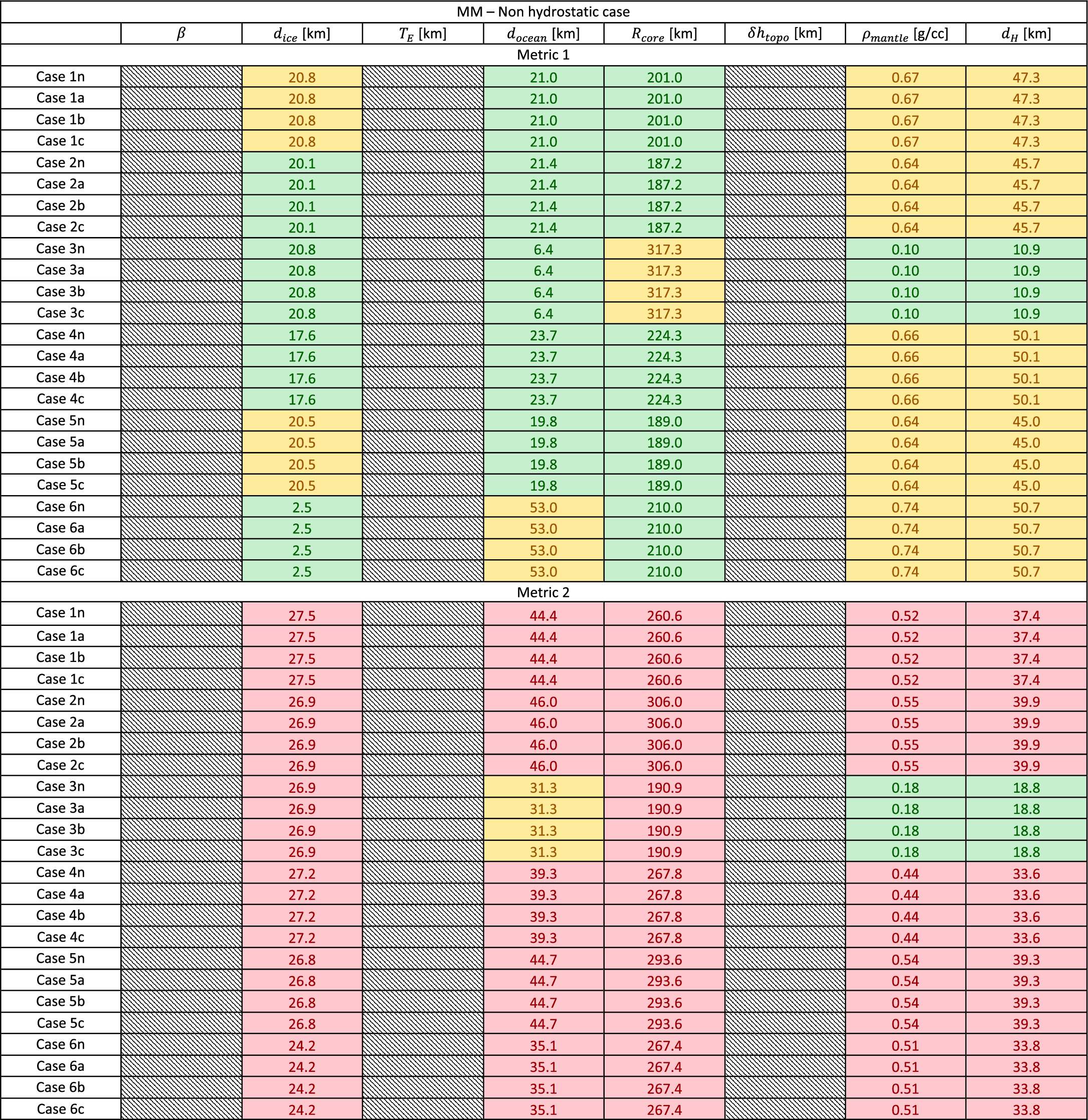
Figure C4. Full results for the MM-Nonhydrostatic case. The numbers and colors follow the same definition as Figures 8 and 9.
Download figure:
Standard image High-resolution image
The numbers and colors reported in the tables follow the same definition as in Figures 8 and 9.
Footnotes
- 5
Rnd7_T3 available at https://naif.jpl.nasa.gov/pub/naif/EUROPACLIPPER/kernels/spk/.
- 6
Note that this definition is more restrictive than the one in Biersteker et al. (2023). They define the M1 Pass criterion based on a 2σ interval.