


Abstract
We update the record of cloud opacity observations conducted by the Mars Science Laboratory (MSL) Curiosity rover to cover the first five Mars Years (MYs) of the mission (Ls = 160° of MY 31 to Ls = 160° of MY 36). Over the three MY period that we add to the previously analyzed two MY record, we achieve good diurnal coverage between 07:00 and 17:00 with nearly 1200 new observations. We derive a new scattering phase function for the clouds of the Aphelion Cloud Belt (ACB) using results from the Zenith and Suprahorizon movie data sets. Our phase function is generally smooth and featureless, which is consistent with the overall lack of atmospheric optical phenomena on Mars aside from a single instance of an observed halo. Applying our new phase function to the data, we find that there is very minimal variability in the ACB's opacity, either diurnally, intraseasonally, or interannually, noting that our observations are only sensitive to ice clouds and cannot detect any ice hazes that may be present over Gale. This contrasts with previous results, which observed a 57% difference in the opacity of morning and afternoon clouds in MY 33. The MY 33 results now appear to be an outlier, not replicated at any point during the MSL mission. We conclude that the higher morning opacities in MY 33 were a consequence of an incomplete understanding of the nature of the scattering phase function close to the Sun.
Export citation and abstract BibTeX RIS

Original content from this work may be used under the terms of the Creative Commons Attribution 4.0 licence. Any further distribution of this work must maintain attribution to the author(s) and the title of the work, journal citation and DOI.
1. Introduction
The Martian climate is dominated by the competing seasonal effects of the planet's obliquity (25 2) and high orbital eccentricity (∼0.0935), which result in significant differences in solar insolation over the course of a year. These differences drive atmospheric processes that divide the Martian year into two halves: the perihelion dusty season and the aphelion cloudy season. Near perihelion, which occurs at a solar longitude (Ls) of 250°, we observe higher atmospheric temperatures and an increase in wind-induced dust lifting off the surface. Near aphelion (Ls = 70°), the atmosphere cools, and we see the formation of an annually repeating feature known as the Aphelion Cloud Belt (ACB; Wolff et al. 1999).
As its name suggests, the ACB is a belt of clouds that encircles Mars, typically between 10°S and 30°N latitude (James et al. 1996). It is a highly repeatable feature (Liu et al. 2003; Tamppari et al. 2003; Smith 2004; Hale et al. 2011), forming each year by Ls = 40°–60° and dissipating around Ls = 150°, with peak optical depths of τvis = 0.2–0.6 occurring near Ls = 100° (Clancy et al. 1996; Wolff et al. 1999). Its formation is driven by the fact that aphelion occurs shortly before the northern summer solstice (Ls = 90°). As the northern hemisphere warms up, the northern polar ice cap begins to sublimate, releasing water vapor into the atmosphere. The cooling atmosphere rapidly becomes saturated with water vapor, leading to the formation of clouds. A similar process does not occur during the southern summer, as the warmer atmospheric temperatures that occur at perihelion prevent the water vapor concentration from reaching the saturation point.
Although the thickness of the ACB peaks around 10°N, the equatorial latitude of the Mars Science Laboratory (MSL) Curiosity rover's landing site (∼46S) allows for observations of the southern edge of the ACB to be conducted from the ground. To take advantage of this fact, a cloud observation campaign has been underway since the first few sols of the mission. Over the course of the mission, the campaign has grown to investigate a number of macro- and microphysical properties of Martian clouds, including their opacities and spacing (Moores et al. 2015; Kloos et al. 2016, 2018), altitudes and angular velocities (Campbell et al. 2020, 2021a), and scattering phase function (Cooper et al. 2019; Innanen et al. 2024).
The primary aim of this paper is to update the cloud opacity analysis performed by Moores et al. (2015) and Kloos et al. (2016, 2018), covering the first two Mars Years (MYs) of the MSL mission (Ls = 160° of MY 31 to Ls = 160° of MY 33; sols 14–1364), to include data taken through the end of MSL's fifth MY on the surface (Ls = 160° of MY 36; through sol 3360). We are particularly interested in examining the diurnal variability reported by Kloos et al. (2018), where the opacity of clouds observed in the afternoon was, on average, about 57% of the opacity of clouds observed in the morning. This difference was attributed to the formation of thick clouds overnight, the remnants of which were observed in the early-morning hours before dissipating by the afternoon. However, because Kloos et al. (2018) only had one MY of full diurnal coverage, it was not possible to determine whether this variability is a persistent feature of the ACB. Now that we have over three MYs of AM/PM coverage, we can finally address this question.
This paper will also supplement the results of Cooper et al. (2019) and Innanen et al. (2024) by examining an alternate means of deriving a scattering phase function for ACB clouds from rover-based observations. The opacities presented by Moores et al. (2015) and Kloos et al. (2016, 2018) were derived assuming that ACB clouds have a constant, flat phase function. However, Cooper et al. (2019) and Innanen et al. (2024) showed that this assumption is only valid beyond a certain scattering angle; closer to the Sun, the phase function deviates significantly from the flat assumption, consistent with the single scattering of light through optically thin clouds. Although the cloud movies that make up the bulk of the observation campaign are specifically intended to look away from the Sun, operational constraints result in their occasional execution outside of their ideal timing windows. When that happens, we observe clouds at scattering angles where the phase function is apparently not flat, invalidating the assumptions made in our model. Consequently, we became interested in examining the extent to which this breakdown affects our opacity results by taking advantage of the known low interannual variability of the ACB to determine our own phase function.
2. Data Sets and Analysis Methods
2.1. The MSL Navigation Cameras
All of the cloud observations to be discussed were taken using MSL's Navigation Cameras (Navcams), of which the rover has two pairs (one pair each for the primary and backup computer systems) mounted to the rover's remote sensing mast (RSM). Although they are classified as engineering cameras, as their primary function is to assist in rover navigation, the Navcams are radiometrically calibrated (Maki et al. 2012) and thus can be used to conduct scientific observations.
The Navcam sensors are flight-ready spare charge-coupled devices left over from the Mars Exploration Rover missions. They have a useful photosensitive area of 1024 by 1024 pixels and have a 45° field of view (FOV). The optical filter bandpass of each Navcam is centered around 650 nm, with sensitivity between 600 and 850 nm. Due to the expected low optical depths of the clouds, the Navcams were selected for the cloud observation campaign over the rover's other cameras due to their superior operational signal-to-noise ratio (S/N > 200:1; Maki et al. 2012), despite being sensitive to a wavelength range that is optimized for observing dust-covered surfaces rather than water-ice clouds. In addition to their excellent S/N, the Navcams provide the widest FOV of any of the rover's cameras (see Figure 1), allowing us to observe clouds over as much of the sky as is possible in a single image.
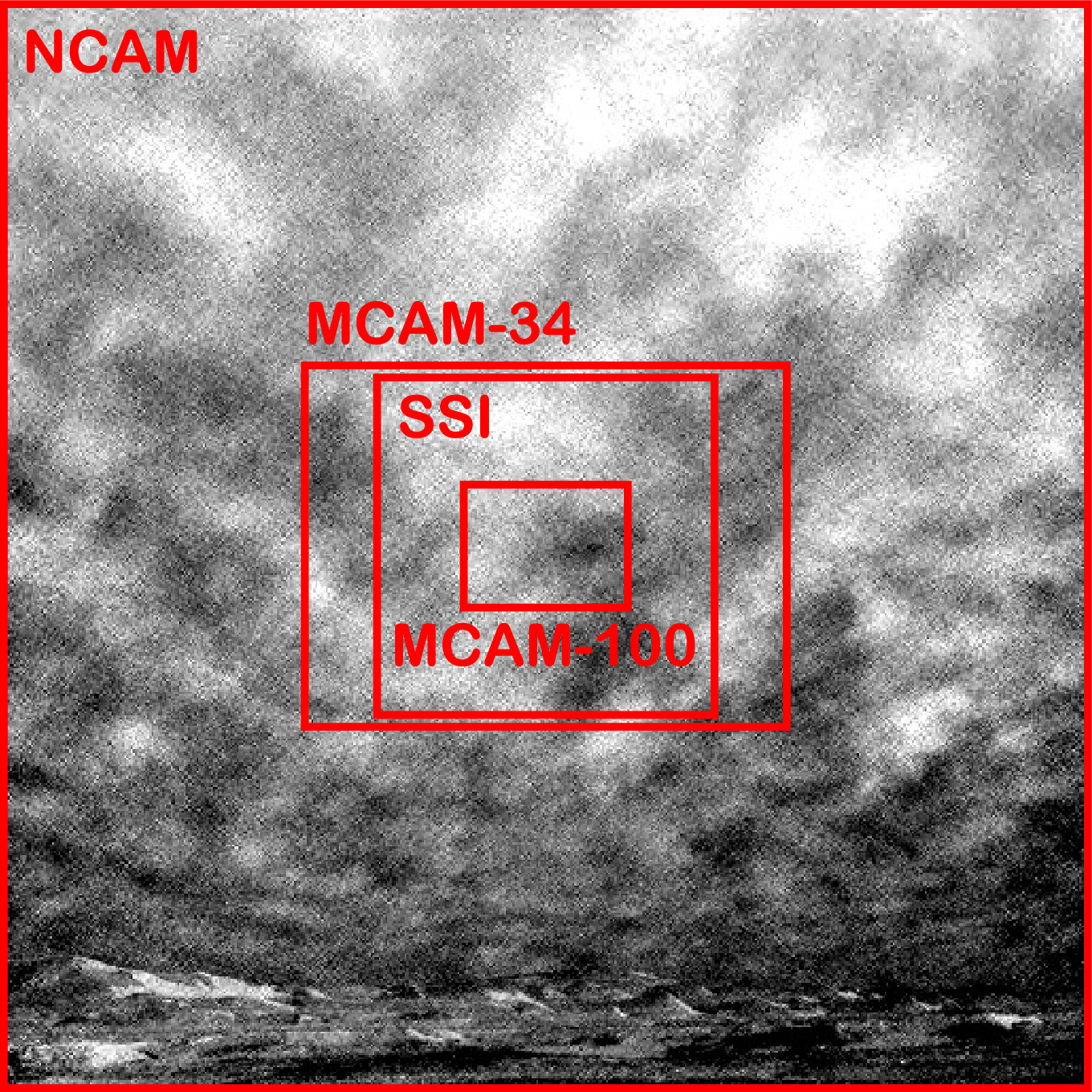
Figure 1. Comparative FOVs of MSL's Navcams (NCAM) and the two Mastcams (MCAM-34 and MCAM-100). Also included for context is the FOV of the Phoenix Surface Stereo Imager (SSI), which Moores et al. (2010) used to observe polar clouds.
Download figure:
Standard image High-resolution image2.2. MSL Cloud Movies
The MSL cloud observation campaign has grown and evolved substantially over the course of the mission, as can be seen in Figure 2. Moores et al. (2015) and Kloos et al. (2016, 2018) all focused on the two longest-running observations: the Zenith and Suprahorizon movies (ZMs and SHMs, respectively). Since the publication of Kloos et al. (2018), a number of new activities have been implemented to study the properties of the clouds over Gale that the ZMs and SHMs are not optimized to observe, such as cloud altitudes and the scattering phase function. An additional two new observations—the Shunt Prevention ENV Navcam Drop-In (SPENDI) and the high data volume SuperSPENDI variant—have allowed us to supplement the nominal SHM cadence.
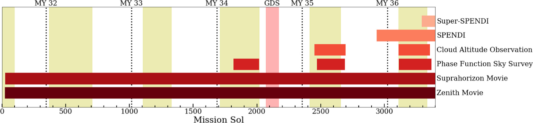
Figure 2. The evolution of the cloud observation campaign over the course of the MSL mission. The ZMs/SHMs and SPENDI/SuperSPENDI observations are taken at all times of year, while the CAO and PFSS are only executed during the ACB season, indicated by the yellow shaded regions. The temporal extent of the MY 34 GDS event is indicated by the red shaded region.
Download figure:
Standard image High-resolution imageIn Figure 3, we present the temporal distribution of the ZMs and SHMs as a function of solar longitude and local true solar time (LTST). From the beginning of the mission until the beginning of MY 33, nearly all ZMs were taken near 16:00 LTST, with the majority of SHMs taken near 12:00 LTST. Both were driven by operational constraints; early-morning observations required additional power to warm the Navcams, while the near-vertical pointing of the ZMs and MSL's equatorial latitude prevent ZMs from being executed within 2.5 hr of local noon due to the risk of having the Sun present in the frame.

Figure 3. Diurnal coverage of the cloud observation campaign over the first five MYs of the mission. The ZM keepout window from local noon is clearly visible, as is the introduction of dedicated AM science time at the beginning of MY 33. Also visible are the gap in coverage around 10:00 LTST caused by the rover's uplink schedule and the gaps that have opened up in MYs 35 and 36 as a result of the rover's age restricting when science block time can be allocated. The ACB season is indicated by the yellow shaded regions, and the red shaded region is the MY 34 GDS.
Download figure:
Standard image High-resolution imageBeginning in MY 33, dedicated once-weekly early-morning science time was allocated for environmental science observations, including a ZM and an SHM. This allowed for nearly full daytime diurnal coverage, with the exception of a gap near 10:00 LTST caused by the rover's uplink schedule. Beginning approximately halfway between the MY 35 and MY 36 ACB seasons, the timing of the AM and noon science blocks has become increasingly constrained, reopening gaps in the diurnal coverage. These gaps are a consequence of the fact that as the plutonium dioxide heat source that powers the rover's radioisotope thermoelectric generator (RTG) decays, simultaneous operation of the rover's survival heaters, actuator and camera warm-up heaters, and science instruments puts a greater strain on MSL's battery resources. Thus, science operations are preferentially limited to times when heating is less of a concern, with less flexibility to deviate from those preferred times than there was in the past.
Because environmental science time is now rarely allocated in the late afternoon, it has become challenging to ensure that our diurnal coverage does not become biased toward the AM and near-noon periods. Since MY 35, we have been aided by the implementation of two new observations—the Cloud Altitude Observation (CAO) and the SPENDI, discussed more in Sections 2.2.1 and 2.2.2, respectively—which contain ZM/SHM observations but are less subject to the power constraints faced by the standard ZM/SHM observations. The CAO is part of the standard ACB season observational cadence and can only be executed in the afternoon, while the SPENDI is specifically designed to drain excess charge from the rover's batteries. The additional flexibility afforded to us by these observations means that we have been able to maintain reasonably robust PM coverage despite the declining output from the RTG.
2.2.1. ZMs
ZMs consist of eight full Navcam frames pointed at an elevation angle of 85°. This near-vertical pointing allows for the determination of quantities such as the angular velocities of clouds (Campbell et al. 2020, 2021b), in addition to cloud opacities. Prior to sol 915, each frame was taken approximately 13 s apart for a total temporal span of 91 s. Beginning on sol 915, the time between each frame was extended to 38 s, bringing the total length of the ZM observation to 266 s. This change was made following an analysis indicating that increasing the interframe spacing improved the observation's sensitivity (Kloos et al. 2016).
Beginning in the MY 35 ACB season, a new cloud observation sequence—the CAO (Campbell et al. 2020)—was implemented that increased the ZM cadence. The CAO is executed once a week between 14:30 and 16:00 LTST during the ACB season and is designed to measure the altitude of clouds passing above the rover. It consists of two movies, one of which is identical to the standard ZMs. This movie, which we refer to as the CAO ZM, can be incorporated into our analysis.
Since Kloos et al. (2018), 508 ZMs have been acquired, including 65 CAO ZMs during the MY 35 and MY 36 ACB seasons, a cadence of approximately one every four sols. Adding the 236 ZMs discussed in previous studies, MSL has taken a total of 744 ZMs in its first five MYs.
2.2.2. SHMs
Since sol 1032, SHMs have been operationally identical to ZMs but pointed at an elevation angle of 26° above the horizon. This lower elevation pointing allows for more robust interpretations of cloud morphologies to be made than is possible with the ZMs, though it presents some challenges as well. Due to the longer path length observed by the SHMs, there is more atmospheric dust between the rover and the clouds. This can reduce the observation's sensitivity, particularly in the bottom half of the frame, where the path lengths are the longest. Additionally, because the Martian surface is variegated on smaller scales and with greater contrast than the sky, the rover's onboard ICER compression algorithm preferentially assigns greater bit depth to surface geology. This means that when nearby terrain appears in the Navcam FOV, as frequently occurs in the SHMs, fine details in the sky (e.g., the clouds we want to observe) are often compressed to a single digital number.
Prior to sol 1032, the operational parameters of the SHMs underwent a number of changes in response to shifting scientific objectives. From the beginning of the mission until sol 594, they looked just above the top of Mount Sharp (1348 azimuth, 385 elevation), with the intent of capturing orographic clouds that are frequently seen forming above topographic peaks. These movies were also downlinked at quarter-resolution (512 by 512 pixels) by implementing two-by-two pixel binning. Beginning on sol 594, the SHM pointing was modified to 1251 azimuth and 10° elevation, and its aspect ratio was changed to 512 pixels wide and 1024 pixels tall. This change allowed the SHM to return a line-of-sight (LOS) extinction value while continuing to search for orographic clouds. Because the increased width doubled the number of pixels in each frame, the decision was made to reduce each movie to four frames, keeping the total data volume constant. The time between each frame was kept the same, cutting the total length of the movie from 91 to 39 s. Analysis of this change uncovered the importance of duration and interframe spacing on observation sensitivity, so on sol 911, the SHM was restored to its original eight frames with a new total length of 266 s, matching the ZMs. To save on data volume, the LOS measurement was split into its own single-frame observation, and the SHMs were brought back to a 512 by 512 pixel resolution. The pointing was also slightly modified to an azimuth of 1346 and 435. By sol 1032, no orographic clouds had been observed over Mount Sharp, so the pointing strategy was changed one final time to what has now been used for >2300 sols. The elevation is fixed at 26°, while the azimuth changes with the seasons (180° from Ls = 0° to 190° and 0° from Ls = 190° to 359°) to avoid pointing the Navcams in the direction of the Sun.
Sol 2937 saw the first execution of a new observation to supplement the SHM cadence. The SPENDI observation was designed as a "shunt prevention" activity to partially drain the rover's battery to prevent it from sitting fully charged for an extended period of time. Each SPENDI takes atmospheric monitoring movies at six pointings, including a north-facing movie pointed at an elevation angle of 15° and a south-facing movie pointed at an elevation angle of 25°. The movies taken at these pointings consist of eight frames taken across 266 s, identical to the standard SHMs. On sol 3346, an enhanced version of the SPENDI observation (SuperSPENDI) was implemented that doubled its data output by taking two movies at each pointing, with 600 s between each movie.
We are adding 669 SHMs to the cloud opacity record, 36 of which are SPENDI or SuperSPENDI observations. This is an average cadence of one SHM every four sols, similar to the ZM cadence. In total, MSL has now taken 941 Suprahorizon or Suprahorizon-like movies.
2.3. Cloud Opacities
Due to the low optical depths of the clouds observed over Gale, they are very rarely visible to the naked eye in the raw movie frames. To enhance the contrast between the clouds and the empty sky for ease of analysis, we use a technique known as mean-frame subtraction (MFS). We first construct a mean frame as a pixel-by-pixel average of all eight frames. This mean frame is then subtracted from each individual frame, leaving behind only the component of the image that varies with time (i.e., the clouds). Although all analysis is performed on the MFS data, we take the additional step of renormalizing each frame by dropping the highest and lowest 2% of the values and stretching the remaining values to assist in the visual identification of cloud features and the selection of high- and low-radiance points for our opacity retrieval models. An example ZM following each of these three steps is shown in Figure 4.
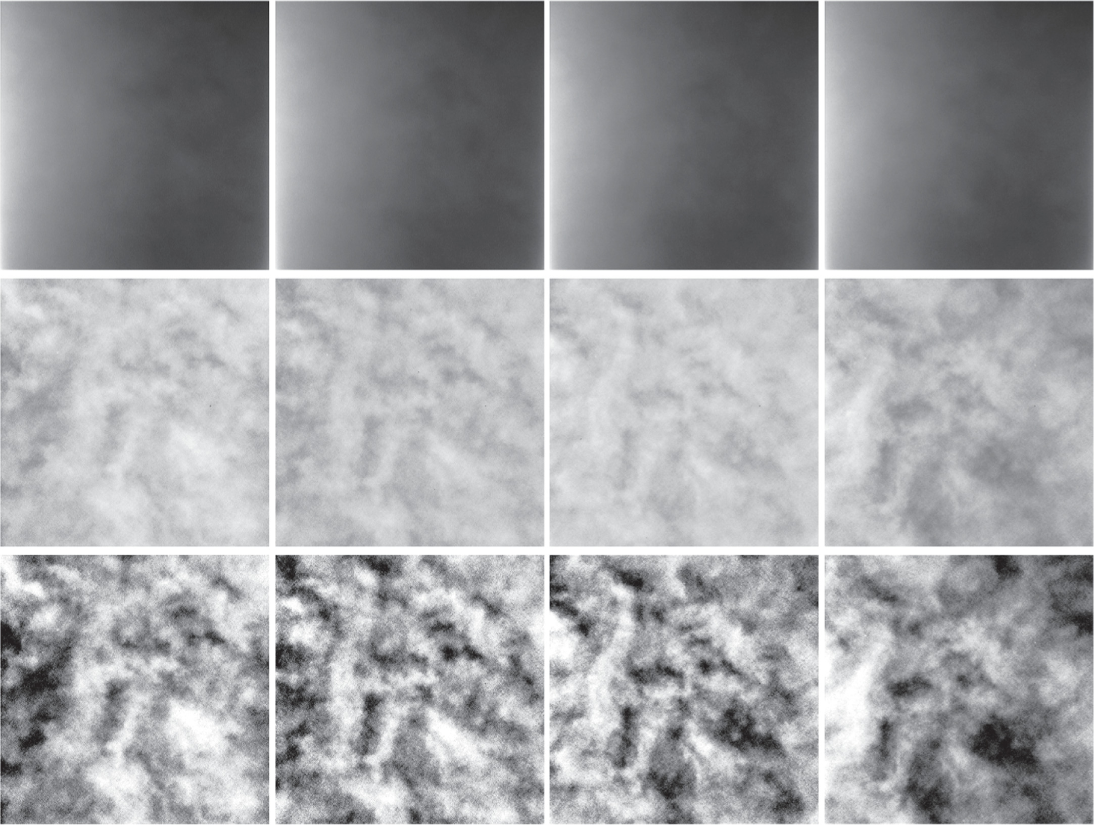
Figure 4. Four frames from a high-quality ZM at three stages in the processing pipeline. In the top row are the raw frames, where the clouds are barely visible. In the middle row, MFS has been applied. The clouds are clearly visible here, but the contrast is still not great. In the bottom row, the middle 98% of the pixel values have been stretched, creating much better contrast between the high- and low-radiance points of each frame.
Download figure:
Standard image High-resolution imageOnce each movie has been processed, it is assigned a quality value between 0 (featureless) and 10 (clouds visible in the raw frames). A value of −1 is also used to indicate movies that are unusable due to either the presence of the Sun in the frame or an RSM failure that left the Navcams pointing in a direction where the sky could not be observed. Movies with quality values of −1 or 0 are excluded from further analysis. In Figure 5, we show the quality values assigned to each movie, averaged across 50 bins of solar longitude and LTST. The ACB season is clearly visible as the band of higher-quality movies between Ls ∼ 50° and 170°. A second, smaller peak centered around Ls ∼ 300° represents the peak of atmospheric dust loading during the perihelion dusty season.

Figure 5. Qualitative movie quality values, averaged across 50 bins of solar longitude and true solar time. Two quality peaks are visible: the ACB between Ls = 50° and 170° and the height of the dusty season near Ls = 300°.
Download figure:
Standard image High-resolution imageTo determine the cloud opacities, we use two models that make different assumptions about the nature of the clouds being observed. The first, reproduced here as Equation (1), is known as the High Clouds (HC) model (see Equations (2)–(9) of Kloos et al. 2016 for a full derivation). The HC model assumes that the clouds are at high altitudes above the bulk of the dust-scattering centers and are composed of water-ice crystals:
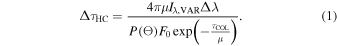
Stepping through this equation term-by-term, μ is the cosine of the zenith viewing angle and Iλ,VAR is the difference in spectral radiance between a high- and low-radiance point in an MFS frame. These two points, corresponding respectively to a cloudy and cloudless portion of the image, are chosen through visual inspection. Note that the low-radiance point could be a region of the sky with lower-opacity clouds rather than open, cloudless sky, so our modeled opacities should be viewed as lower limits. Δλ is the spectral bandpass of the Navcams (250 nm), P(Θ) is the scattering phase function of the clouds, F0 is the in-band solar flux at the top of the atmosphere, and τCOL is the atmospheric column density as measured by Mastcam imaging of the solar disk (Lemmon et al. 2024).
For an in-depth discussion of the uncertainties involved in the HC model, refer to Kloos et al. (2018). Here, we will note that the largest uncertainty comes from P(Θ), as the scattering phase function of Martian clouds is poorly constrained. Previously, Moores et al. (2015) and Kloos et al. (2016, 2018) assumed that this term was fixed at a constant value of 1/15. This assumption was justified as being representative of the flat phase function of terrestrial cirrus clouds at large scattering angles (Wang et al. 2014) and was verified by comparing the opacities derived from ZMs and SHMs taken less than 10 minutes apart. These movie pairs observe the same cloud at scattering angles up to 30° apart, and no significant difference in opacity was observed in all but three pairs (Kloos et al. 2018).
Despite the apparent validity of the flat phase function assumption in the scattering angle regimes explored in the literature to date, we will not be adopting this assumption because the MY 34–36 data set covers a wide range of scattering angles (16°–142°; see Figure 6). Previous studies using MSL data (Cooper et al. 2019; Innanen et al. 2024) have shown that the scattering phase function of ACB clouds over Gale deviates significantly from a flat curve at low scattering angles near the Sun, indicating that continued use of this assumption is not appropriate at low scattering angles. Kloos et al. (2016) determined a lower limit for the scattering phase function using the ZMs and SHMs but was limited to scattering angles between 70° and 115°, with the bulk of the observations between 80° and 90°. These values are outside the range where the value of the phase function is expected to deviate from the flat assumption. Their analysis was also limited by the availability of Mars Climate Sounder (MCS) cloud opacity retrievals to use as a reference, which cut the number of useful data points down to 12 ZMs and 8 SHMs.

Figure 6. Frequency of the scattering angles where clouds were observed during MYs 34–36, in 10° bins. Nearly all observations took place at scattering angles between 20° and 120°, which is a much wider range than was previously explored by Kloos et al. (2016, 2018). The increased number of observations at small scattering angles (close to the Sun) relative to MYs 31–33 is of particular interest since that is the regime in which Cooper et al. (2019) and Innanen et al. (2024) suggest that the scattering phase function deviates significantly from the flat, constant assumption used in the past.
Download figure:
Standard image High-resolution imageThe second model, reproduced here as Equation (2), is known as the Whole Atmosphere (WA) model (see Equation (3) of Moores et al. 2010 for a full derivation). It assumes that the clouds are at lower altitudes and have similar scattering properties as the bulk atmosphere (i.e., are dust-based rather than ice-based):

Here, a is Iλ,VAR (as in the HC model) divided by the mean radiance of the frame.
Given the assumptions made by these models, it is most appropriate to use the HC model during the ACB season, when we are most likely to be observing high-altitude water-ice clouds, and the WA model at all other times of year, when we are most likely to be observing lower-altitude dust clouds. To determine the temporal extent of the ACB, we adopt the same approach as Moores et al. (2015) and Kloos et al. (2016, 2018). The Mars Color Imager (MARCI) instrument on board the Mars Reconnaissance Orbiter (MRO) produces weekly weather reports, which we monitor for the presence of ACB clouds. During the study period covered here, there was one extended gap in MARCI coverage, lasting from Ls ∼ 75° of MY 35 to Ls ∼ 125° of MY 36. This covers the end of the MY 35 ACB season through the beginning of the MY 36 ACB season. As we are thus unable to determine when the MY 35 ACB season ended and the MY 36 ACB season began using orbital data, we instead adopt the range of solar longitude values where ACB clouds are most typically observed: Ls = 40°–150° (Kloos et al. 2018). We note that in MYs 32, 34, and 35, ACB clouds were observed by MARCI as soon as Ls = 10°–30°, so setting the beginning of the MY 36 ACB season at Ls = 40° may be later than is appropriate.
Because we are most interested in ACB clouds, the remainder of this paper will be focused on the values derived using the HC model. Comparisons between ACB HC values and non-ACB WA values are restricted to Figure 12 and Table 1.
Table 1. Mean Opacities for ACB and Non-ACB Clouds, Divided by Mars Year
| Mean Preferred | Mean Preferred | ||
|---|---|---|---|
| Ls | Mars | Cloud Opacity | Cloud Opacity |
| (Range) | Year | (ZMs) | (SHMs) |
| ACB | |||
| 160°–207° | 31 | 0.05 ± 0.03 | 0.09 ± 0.04 |
| 10°–172° | 32 | 0.07 ± 0.04 | 0.06 ± 0.03 |
| 42°–146° | 33 | 0.11 ± 0.08 | 0.18 ± 0.10 |
| 12°–157° | 34 | 0.12 ± 0.07 | 0.13 ± 0.07 |
| 28°–163° | 35 | 0.12 ± 0.07 | 0.11 ± 0.08 |
| 41°–148° | 36 | 0.10 ± 0.07 | 0.11 ± 0.07 |
| Non-ACB | |||
| 208°–9° | 31/32 | 0.006 ± 0.002 | 0.006 ± 0.002 |
| 173°–41° | 32/33 | 0.005 ± 0.005 | 0.004 ± 0.002 |
| 147°–11° | 33/34 | 0.010 ± 0.006 | 0.005 ± 0.002 |
| 158°–27° | 34/35 | 0.008 ± 0.001 | 0.004 ± 0.001 |
| 164°–40° | 35/36 | 0.009 ± 0.003 | 0.008 ± 0.005 |
Note. The solar longitude range of each period is also indicated. Note the generally low interannual variability.
Download table as: ASCIITypeset image
2.4. Determining the Scattering Phase Function
We can invert Equation (1) to solve for the scattering phase function rather than the opacity:

Rather than assuming a value for the scattering phase function, we now have to assume a value for the cloud opacity. Kloos et al. (2016) used this form of the HC equation along with water-ice optical depth retrievals from MCS and the ZMs and SHMs taken during the first MY of the MSL mission to determine a lower limit for the scattering phase function across a narrow range of scattering angles (70°–115°). MCS water-ice optical depths were also been used by Cooper et al. (2019) and Innanen et al. (2024) in combination with a dedicated observation known as the Phase Function Sky Survey (PFSS) to determine the value of the scattering phase function across a much wider range of scattering angles (20°–150°), though the PFSS produces increasingly unreliable results for scattering angles below approximately 45°.
Using optical depths from MCS is potentially problematic for several reasons. First, MCS has difficulty retrieving values near the surface due to increased dust opacity in the lower atmosphere, with the water-ice column depths often limited to altitudes above 30 km (Guzewich et al. 2017). The clouds we observe over Gale Crater are frequently lower than that (Campbell et al. 2020, 2021a), so MSL and MCS may not be observing the same clouds. Indeed, we know that MCS and MSL are not observing exactly the same clouds, as MCS measurements are not taken simultaneously with the ZMs/SHMs/PFSS. Second, MRO, to which MCS is mounted, is in a Sun-synchronous orbit, meaning that it observes each part of the surface at the same time each day. Kloos et al. (2018) suggested that cloud opacities over Gale vary diurnally, so the MCS data would not capture this detail. Furthermore, the footprint of MCS measurements is quite large, with typical nadir observations having a horizontal resolution of 1–6 km (Hayne et al. 2012) and typical limb observations having a much worse horizontal resolution of 200 km (McCleese et al. 2007).
Ideally, we would like the opacity input to Equation (3) to be derived from observations taken of the same clouds that we see from MSL. If it is indeed the case that the flat, constant phase function assumption holds at large scattering angles, then we can assume that the opacities calculated using Equation (1) in that regime are representative of opacities at all scattering angles. To account for potential diurnal or interannual variability in opacities, we can split the observations taken in the flat phase function regime by MY and time of day, then use an average of each as an input to Equation (3) to determine the phase function at all observed scattering angles.
To ensure a consistent methodology across all observations taken to date, we will need to apply our new phase function to the previously published data sets. Unfortunately, neither Moores et al. (2015) nor Kloos et al. (2016, 2018) documented the specific points selected for analysis in each movie. However, the instrument pointing is recorded in the Planetary Data System (PDS) label for each observation, so we can determine the scattering angle at the center of the frame. The wide FOV of the Navcams means that the actual scattering angle observed can differ by up to 30° from this central value. If we assume that the highest-contrast points in the MY 32 and 33 data occurred near the Sun and close to the edge of the Navcam frame, as was frequently the case in the MY 34–36 data, we can apply a ∼20° correction to the central scattering angle as a reasonable guess for what the true observed scattering angle was. Doing so, we find that the dependence of the opacity on scattering angle for MYs 32 and 33 (assuming a flat phase function) is nearly identical to that in MYs 33–36 (see Figure 7). In MY 33, nearly all of the high-opacity, low scattering angle observations were taken in the morning, suggesting that if a proper phase function correction was to be applied to these data, the Kloos et al. (2018) diurnal variability would likely be much smaller than what was reported, if it is present at all.

Figure 7. Moving averages of the uncorrected (flat phase function) opacity data, split between the previously published MY 32 and 33 ACB seasons and the newly analyzed MY 34–36 seasons from this paper. In the top panel, the MY 32 and 33 data are presented using the scattering angle at the center of the Navcam frame, while in the bottom panel, we apply a 20° correction, typical of the angular distance between the center and analyzed points in the MY 34–36 data. Once this correction has been applied, we see that the dependence of opacity on scattering angle caused by the assumption of a flat phase function is nearly identical between the two data sets. This suggests that the application of the flat phase function assumption in previous studies was inappropriate.
Download figure:
Standard image High-resolution image3. Results
3.1. The Scattering Phase Function
In Figure 8, the problems resulting from the flat phase function assumption are immediately obvious. Typical water-ice phase functions peak strongly in the forward-scattering direction, meaning that they would have values higher than the previously assumed 1/15. Because the phase function appears in the denominator of Equation (1), having a smaller value for the phase function will result in a higher value for the opacity, leading to a nonphysical increase in opacities at scattering angles below approximately 60°.
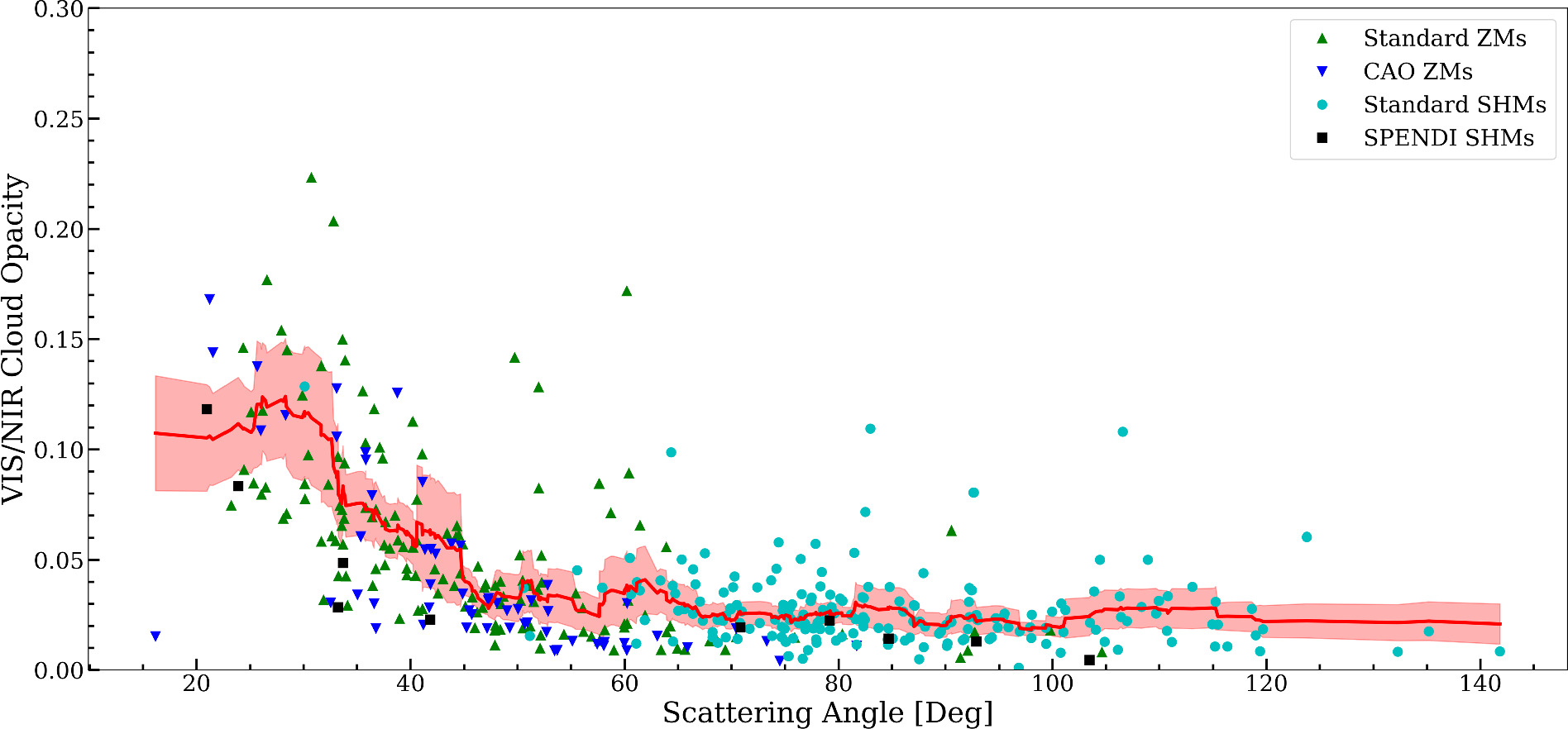
Figure 8. HC opacities as a function of scattering angle if the assumption of a flat phase function is used. The red line is a moving average with the associated 95% confidence interval. There is a clear, nonphysical upward trend in opacities sunward of approximately 60°, indicating that the flat phase function assumption is inappropriate in this regime. We have also indicated the movie type of each measurement to show that ZMs are more likely to observe low scattering angles than SHMs.
Download figure:
Standard image High-resolution imageBased on the results seen in Figure 8, we decided to set the minimum cutoff for determining the "true" opacity at a scattering angle of 70°. The average of the values further from the Sun than this cutoff (after splitting by MY and time of day) were used as the opacity input to Equation (3) when deriving the phase function.
Our six derived phase functions are presented in Figures 9 and 10, divided by MY and time of day, respectively. The phase function curves and associated 95% confidence intervals were found using a sliding average with a window size of 5°. In general, the phase functions behave as we expect: flat at high scattering angles and increasing as the measurements approach the Sun. This is qualitatively similar to the phase functions derived by Cooper et al. (2019) and Innanen et al. (2024), as well as to observed phase functions of terrestrial cirrus clouds (Wang et al. 2014). The MY 34 AM and PM phase functions cover a similar range of scattering angles, but this is not the case for MYs 35 and 36, whose AM phase functions extend approximately 40° and 20° further from the Sun, respectively, than their PM counterparts. These unusually high scattering angle observations are a combination of SHMs that were taken in the very early morning (before 06:30 LTST) and those that had their azimuthal pointing adjusted to avoid looking at high-elevation local terrain features, consequently observing an area of the sky further from the Sun than usual.
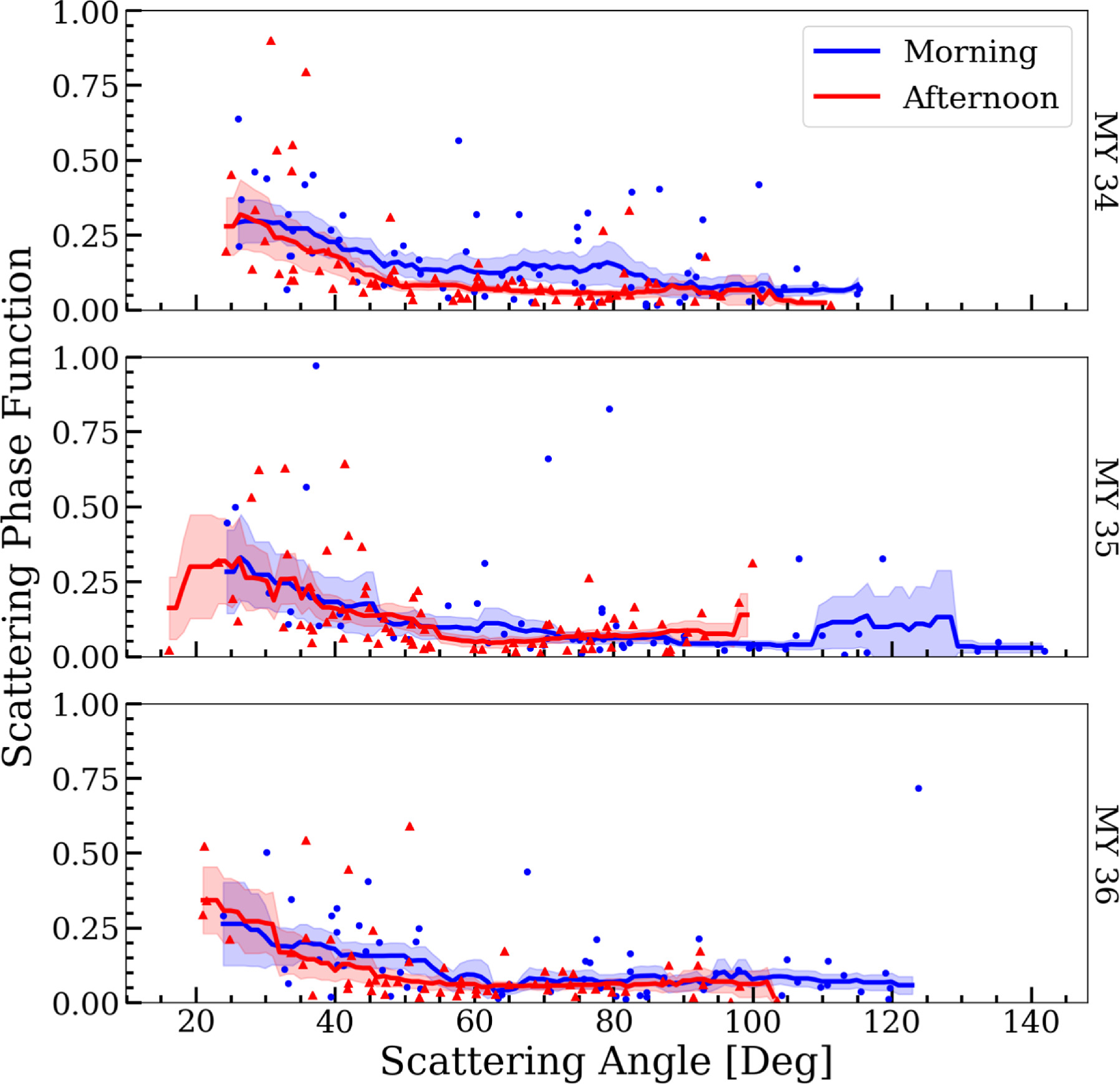
Figure 9. Looking for diurnal variability in the scattering phase function by comparing AM and PM phase functions for MYs 34–36. The shaded regions represent the 95% confidence interval of the moving average. There does not appear to be any significant difference between the AM and PM phase functions in any year, consistent with the findings of Innanen et al. (2024).
Download figure:
Standard image High-resolution image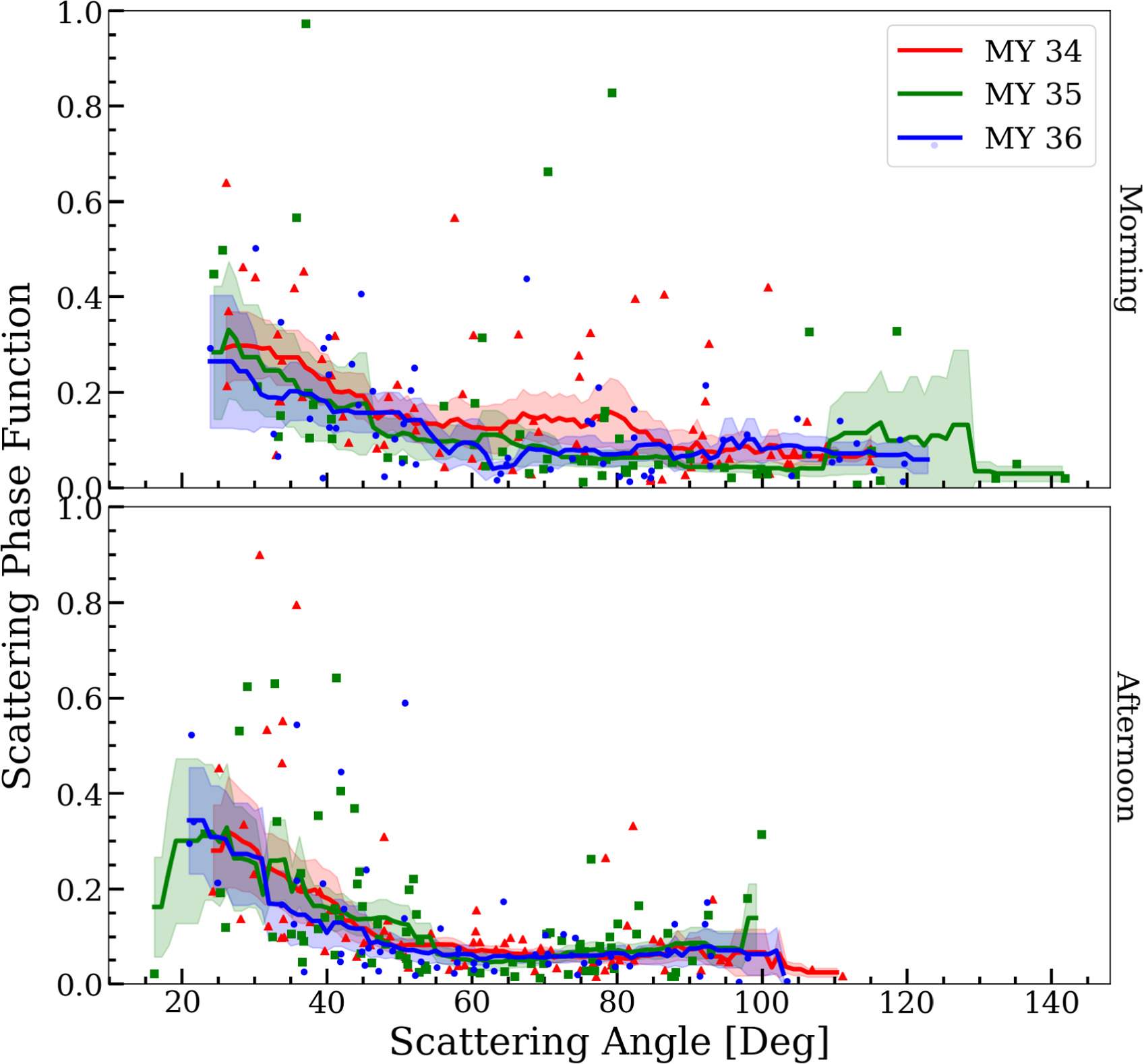
Figure 10. Examining interannual variability in the scattering phase function by comparing the AM and PM phase functions across MYs 34–36. We see relatively close agreement between the three MYs for which a phase function was derived, leading us to conclude that there is no meaningful interannual variability in the shape of the phase function.
Download figure:
Standard image High-resolution imageThere does not appear to be any significant interannual or diurnal variability in the phase functions, as the curves for all 3 yr lie within the 95% confidence interval of the other 2 yr. This is consistent with other work undertaken on MSL that found no significant variability in the phase function of water-ice clouds over Gale (Innanen et al. 2024).
Because we do not see any significant interannual or diurnal variability in the shape of the scattering phase function, we assume that all clouds observed during the MY 34–36 ACB seasons have the same phase function and thus adopt a single phase function for all years at all times of day.
Before our phase function can be used in the HC model, it must be normalized. Traditionally, phase functions are normalized to a value of either 4π or 1. However, because our observations do not cover the full range of scattering angles, it is not possible for us to normalize our phase function on its own. Instead, it is normalized to a set of analytically derived phase functions. For a full discussion of the normalization procedure used, see Section 4.4.
3.2. Cloud Opacities
Cloud opacities for the MY 34–36 ACB seasons are presented in Figure 11 as a function of scattering angle, solar longitude, and LTST, along with the values derived using the flat phase function assumption. As expected, the magnitude of the difference is largest at small scattering angles and for ZMs taken close to the ZM keepout window.

Figure 11. Comparing the calculated cloud opacities before (red) and after (black) applying the phase function correction as a function of scattering angle (top panel), solar longitude (middle panel), and LTST (bottom panel). In the top panel, we can see that the near-Sun increase (also shown in Figure 8) goes away after applying the correction.
Download figure:
Standard image High-resolution imageIn Figure 12, we present all measured cloud opacities from MYs 31–36. In Table 1, we present the mean preferred cloud opacities for the ZMs and SHMs, as well as the Ls ranges over which each method was applied. The HC opacities during the ACB season are much higher than the WA opacities during the dusty season, which is consistent with the lower-quality values seen in Figure 5. In reality, the transition between the two regimes is unlikely to be as abrupt as it is portrayed here. However, because we do not have the ability to distinguish between water-ice and dust clouds, we cannot model a transitional period when both dust and water-ice clouds might be observed.
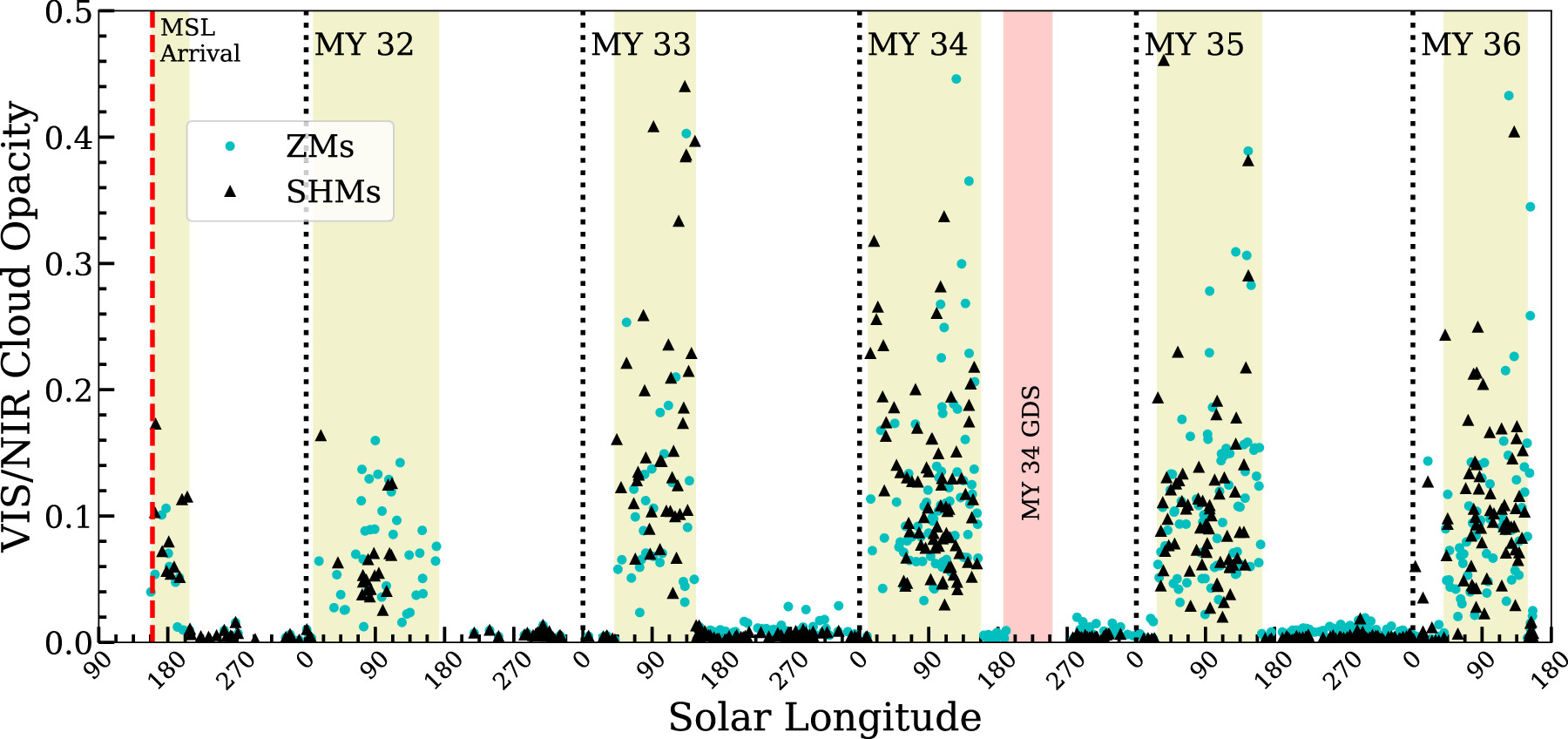
Figure 12. Derived opacities for all movies with visible clouds, combining data from this paper, Moores et al. (2015), and Kloos et al. (2016, 2018). The cyan circles are ZMs, and the black triangles are SHMs. The yellow shaded regions indicate the solar longitude ranges of the ACB, and the red shaded region is the MY 34 GDS event. We can see that ZMs generally have higher opacities than SHMs, particularly outside of the ACB season, consistent with their greater sensitivity to clouds. The notable exception is MY 33, where the SHMs consistently recorded opacities that were much higher than those seen by Curiosity in other years.
Download figure:
Standard image High-resolution image3.3. Diurnal and Interannual Variability of Opacities
The early-morning science blocks that were first implemented during MY 33 have continued through MY 36, so we now have four full MYs of good diurnal coverage from 06:00 to 18:00 LTST. As was the case in Kloos et al. (2018), the gap in diurnal coverage near 10:00 LTST due to rover uplink activities persists. In MY 36, an additional coverage gap emerged near 14:00 LTST, with many fewer observations taken near that time than in previous MYs due to operational constraints imposed by the rover's age.
In the left panels of Figure 13, we present the opacities as a function of LTST, averaged across half-hour bins. There does not appear to be any obvious diurnal variability. MYs 33 and 34 do have a larger number of high-opacity movies in the morning, but these observations are outliers; the bulk of the clouds observed in the morning during these 2 yr are similar to those observed in the afternoon. Consequently, we conclude that while high-opacity clouds may be more common in the morning, there is no systematic difference in the opacity of morning and afternoon clouds over Gale.
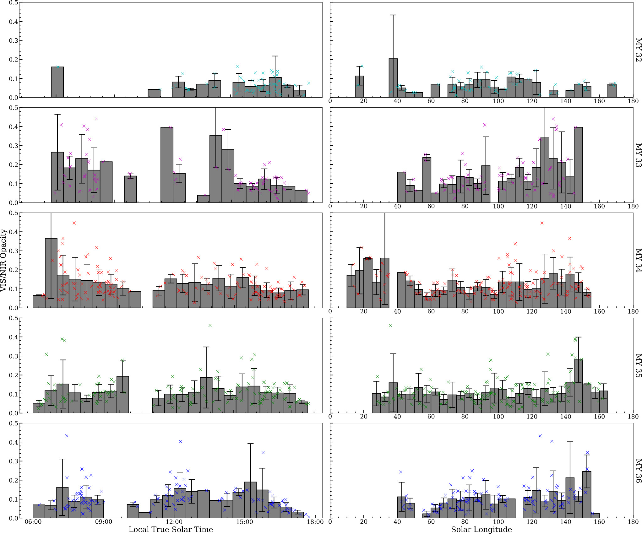
Figure 13. Left panels: ACB cloud opacities for MYs 32–36 as a function of LTST, averaged across bins of 30 minute lengths. Individual observations are indicated by the colored markers. There does not appear to be any meaningful variability, either across the whole day or comparing AM and PM values. The apparent drop-off in opacities near sunrise and sunset is an illumination effect caused by the limitations of our simplified radiative transfer model rather than an actual change in opacity. Right panels: ACB cloud opacities for MYs 32–36, averaged across 5° solar longitude bins. Individual observations are indicated by the colored markers. There is no clear intraseasonal variability, though MYs 35 and 36 do have slightly higher opacities near Ls = 140°.
Download figure:
Standard image High-resolution imageThese results suggest that the variability reported by Kloos et al. (2018) is likely the result of the scattering angle effect demonstrated in this paper rather than a true difference in opacity. Unusually, the highest-opacity outliers in MY 33 were almost all SHMs. Because the SHMs are pointed at a more oblique angle than the ZMs, there is a longer physical distance between the rover and the clouds being observed. Consequently, we are looking through more atmospheric dust, which tends to lower the sensitivity of the observation. This effect can be seen most acutely during the non-ACB season, when the ZMs regularly record higher opacities than the SHMs taken at the same time (note in Figure 12 how the ZM observations clearly lie above the SHM observations).
There is a slight drop in opacity near both sunrise and sunset, but this is an illumination effect rather than a true change in opacity. When the Sun is near the horizon and the sky is darker than it is with the Sun at high elevation angles, the contrast between the clouds and the background sky decreases, lowering the value of Iλ,VAR for a given opacity. Properly addressing cloud opacities at these times of day will likely require a 3D radiative transfer model, which is beyond the scope of this paper.
Following the analysis of Kloos et al. (2018), we averaged our opacities into bins of width 5° Ls to examine variability across the temporal extent of each ACB season (the right panel of Figure 13). There appears to be no meaningful variability during the MY 34 ACB season, while both the MY 35 and MY 36 seasons have a peak near Ls = 140°–160°. However, the MY 36 peak is likely due to there being a small number of data points in that bin, one of which is a high-opacity outlier. We do not observe the Ls = 50°–90° peak seen by Kloos et al. (2018) in MY 33, which was attributed to the rapid transport of water vapor to cloud-forming altitudes by the Hadley cell winds, whose velocities reach their maximum near this time (Wolff et al. 1999).
4. Discussion
4.1. The Phase Function Effect
We assumed that the "true" cloud opacity clusters around the average value of the measurements made at scattering angles >70°, so there is some circular reasoning in then concluding that there is no variability. We did attempt to account for potential diurnal and interannual variability by deriving a separate phase function for each MY and time of day, but there is more that we can do to justify this assumption.
To do so, we repeated our analysis using just those points that lie in the regime where the flat phase function assumption is valid, without applying our derived phase function correction. The results of this analysis are shown in Figure 14. Due to the smaller number of data points (many bins only have one or two observations), it is harder to draw robust conclusions, but there is no obvious variability, either diurnally, intraseasonally, or interannually. As such, we conclude that the observed low variability is a real feature and not a product of our assumptions.
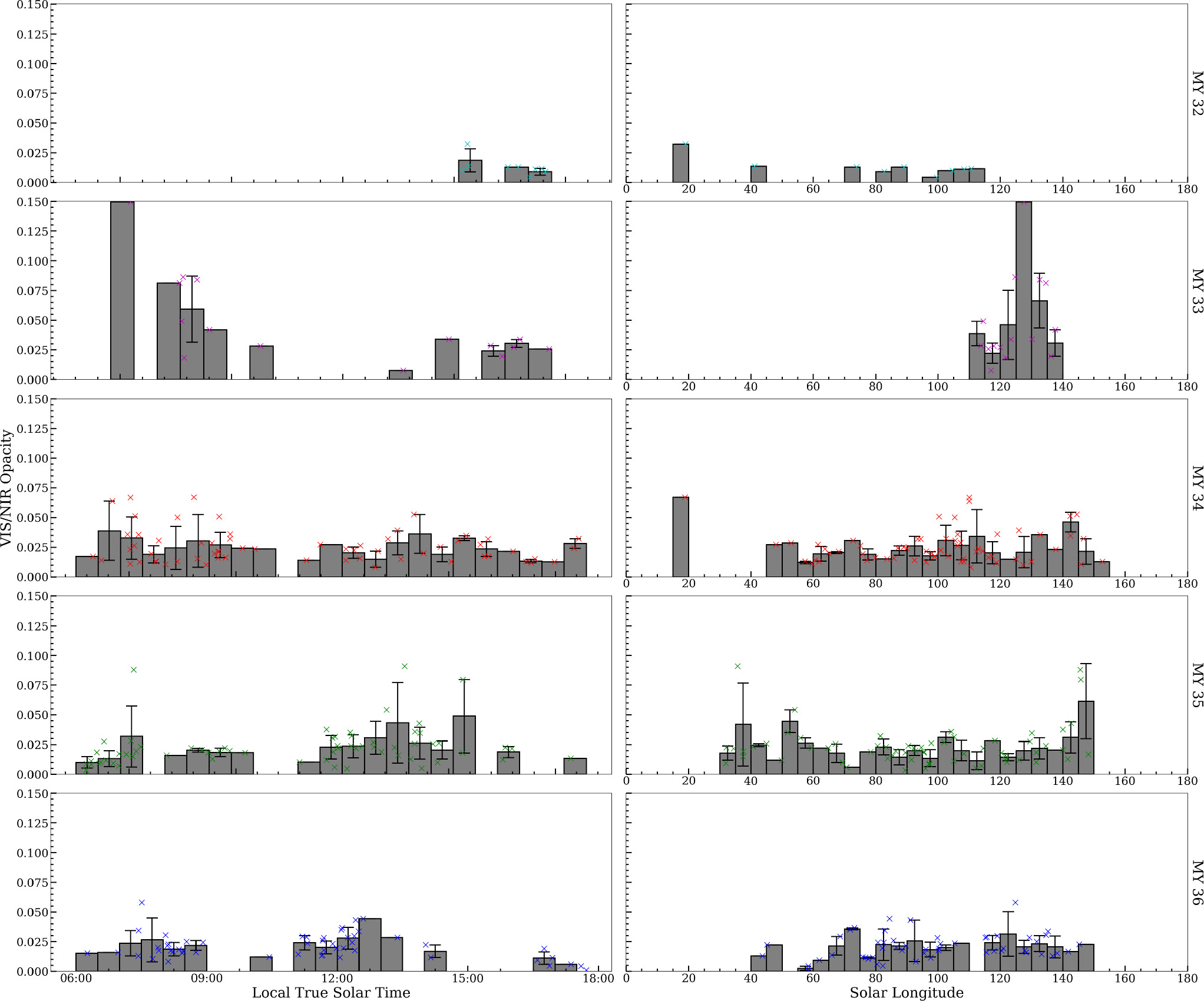
Figure 14. ACB cloud opacities for MYs 34–36, averaged across bins of 30 minutes (left) and 5° solar longitude (right). Individual observations are indicated by the colored markers. Here, we have removed the phase function correction, as well as all points taken at scattering angles <70°. The smaller number of data points in each bin compared to Figure 13 makes a robust analysis more difficult, but there is no obvious diurnal or seasonal variability. This suggests that the observed low variability in Figure 13 is real and not an effect of the assumptions we made when applying the phase function correction.
Download figure:
Standard image High-resolution image4.2. Diurnal Variability
The apparent lack of diurnal variability in the opacity of ACB clouds over Gale is unusual in the global context. There is substantial evidence suggesting that Martian cloud formation is driven at least in part by thermal tides (e.g., Hinson & Wilson 2004; Szantai et al. 2021), implying that we would expect to observe diurnal changes in opacity. Indeed, diurnal variability in Martian aerosols has been previously documented, e.g., over Tharsis (Madeleine et al. 2012) and Jezero (Patel et al. 2023; Smith et al. 2023). The most frequently observed pattern is an enhancement in the early morning, attributed to fogs that form overnight, and a smaller enhancement in the early afternoon, potentially due to increased dust lifting activity delivering more cloud condensation nuclei to cloud-forming elevations (Tamppari et al. 2003).
However, these patterns are not necessarily consistent across the entire planet. Recent analysis of ACB optical depths retrieved by the Emirates Mars Infrared Spectrometer (EMIRS) on board the Emirates Mars Mission (EMM) orbiter has shown that while the double-peaked pattern with maxima in the early morning and late afternoon with a midsol low are observed over much of the spatial extent of the ACB, the magnitude of the differences can vary significantly from location to location, with some areas showing little to no diurnal variability (Atwood et al. 2022). The largest differences (Δτ ∼ 0.1–0.2) are seen over Tharsis and the northern midlatitudes, while the southern edge of the ACB (i.e., where MSL is located) experiences less variability between morning and afternoon clouds, similar to what we have observed. It should be noted that the EMIRS data do still show decreased cloud opacities near local noon in the vicinity of Gale (albeit a smaller difference than elsewhere on the planet), which we do not observe.
4.3. Comparison with MARCI/Emirates Exploration Imager Water-ice Opacities
To validate our opacity retrievals, we can compare them with those from orbital spacecraft. For this purpose, we use retrievals from MARCI on board MRO and from the Emirates Exploration Imager (EXI) on board the EMM Hope probe. The retrieval pipelines for these data sets are described in Wolff et al. (2019, 2022), respectively.
Because MRO is in a Sun-synchronous orbit, MARCI observes all points on the surface at approximately the same local time (∼15:00 LTST, though the exact time can vary significantly across a single MARCI observation due to the instrument's large FOV). As such, the MARCI retrievals cannot capture any diurnal variability, but they can still be used to assess intraseasonal and interannual variability.
Unlike MRO, EMM is in an elliptical supersynchronous orbit, which allows for observations of the surface to be carried out at different local times, albeit with varying resolutions as the spacecraft's altitude changes. This means that EXI optical depths can be used to validate our claim of low diurnal variability over Gale. However, we can only directly compare with MY 36, as EMM arrived at Mars shortly after the beginning of MY 36.
Both data sets are of sufficiently high resolution that it would be inappropriate to extract the pixel value immediately over the rover, particularly for the SHMs. Depending on the altitude of the clouds (15–30 km during the ACB season; Campbell et al. 2020), the clouds seen in the SHMs may be as far as ∼290 km away from the rover, well outside of Gale (see Figure 15 for an example). As such, selecting the cloud opacity retrieved from immediately over the rover may not be representative of the cloud opacities retrieved from our movies, as the two retrievals would come from clouds with significant spatial separation. To account for this, we adopt the average of all MARCI/EXI pixels within the Navcam FOV as our comparison data set.
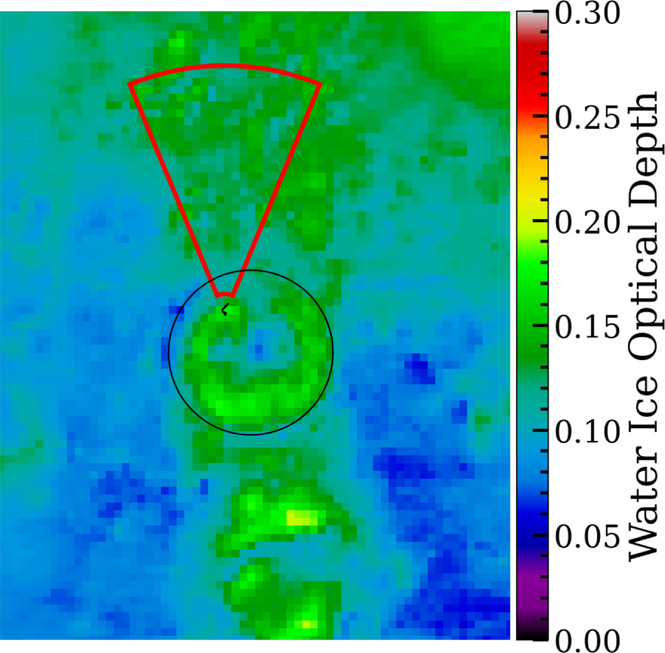
Figure 15. The FOV captured by a north-facing SHM (in red) assuming a cloud altitude of 22.5 km overlaid on top of a MARCI water-ice optical depth map. The black circle marks the rim of Gale, while the black line within Gale is the MSL traverse. The Navcam FOV captures clouds in a large area with a range of optical depths.
Download figure:
Standard image High-resolution imageThe results of these comparisons can be seen in Figures 16 (MARCI) and 17 (EXI). Our opacity retrievals closely track the orbital measurements; we particularly note the increase in opacities near the end of the ACB season (Ls = 150°) in MY 35 and the slight dip near Ls = 60° in MY 36.
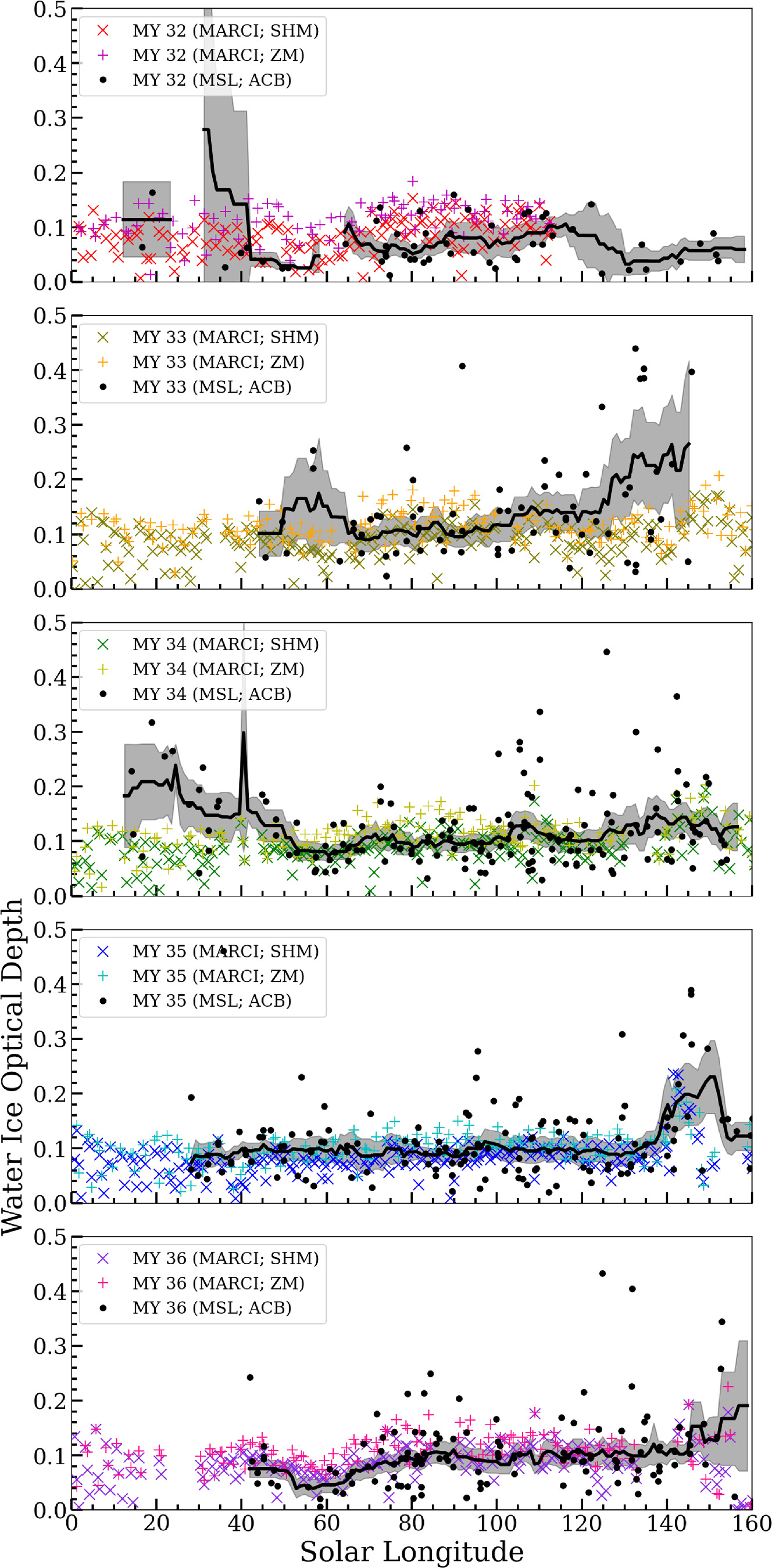
Figure 16. Comparisons between MARCI and MSL water-ice retrievals for MYs 34–36. The MSL retrievals generally track those from orbit, with deviations occasionally seen near both the beginning and end of the ACB season, possibly indicating the presence of more dust in the atmosphere at these times than at the peak of the ACB season.
Download figure:
Standard image High-resolution image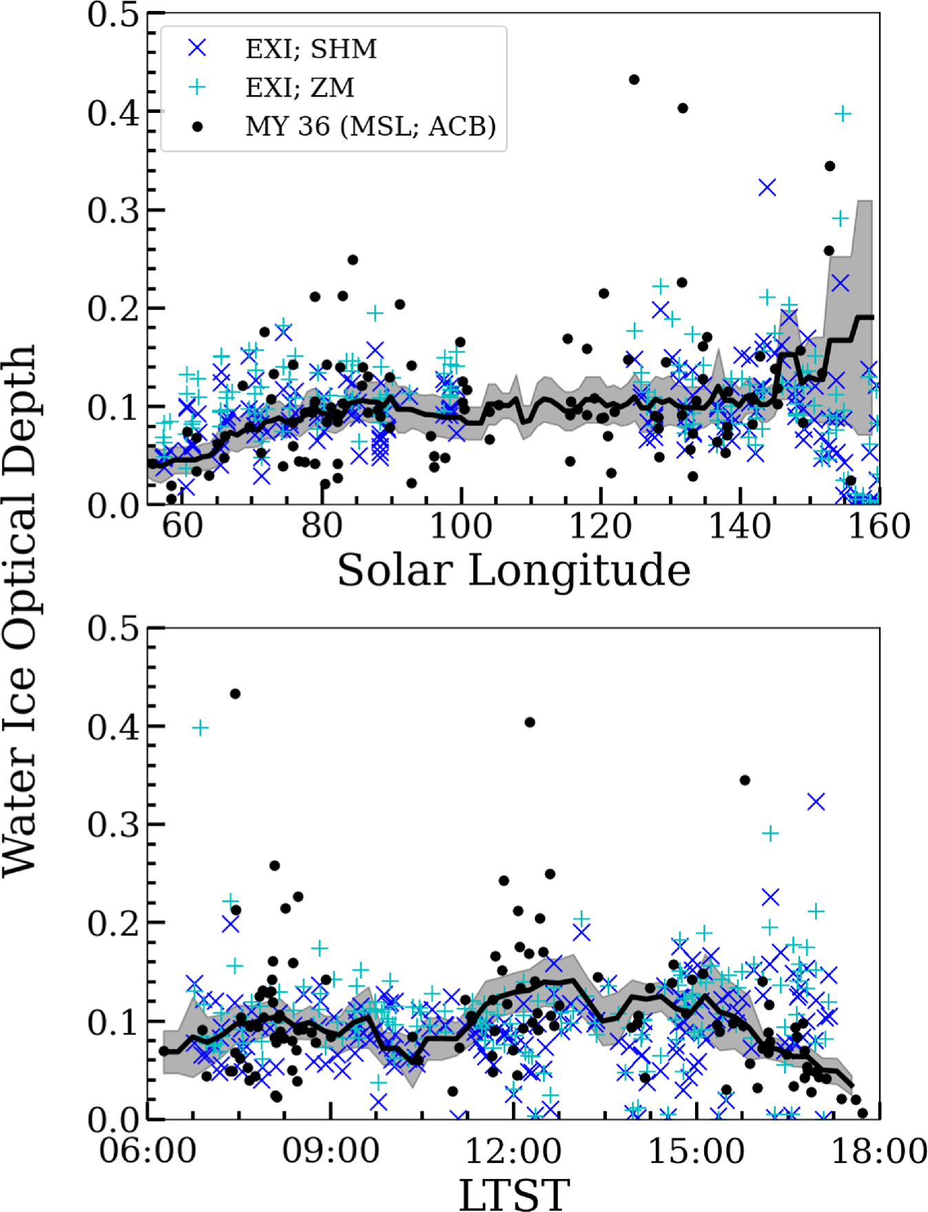
Figure 17. Comparisons between EXI and MSL water-ice retrievals for MY 36 as a function of solar longitude (top) and LTST (bottom). As with the MARCI data, the MSL retrievals are flatter (in solar longitude) and lower magnitude than the EXI retrievals, though the EXI data are subject to the same surface reflectance problem as the MARCI data, as the ZM averages are higher than the SHM averages. However, we do see that EXI does not appear to observe any meaningful diurnal variability during the ACB season, other than a potential slight enhancement in the very early morning and late evening. This low diurnal variability is consistent with what we observe with MSL.
Download figure:
Standard image High-resolution imageOur ground-based retrievals occasionally experience upward deviations from the orbital retrievals near the beginning and end of the ACB season. This may indicate increased atmospheric dust loading at these times of year, as we are not able to distinguish between water-ice and dust clouds, while the MARCI and EXI retrievals can. This is particularly noticeable at the end of the MY 36 ACB season, when an early-forming regional dust storm swept over Gale.
In MY 32 and MY 36, it appears that our derived opacities are slightly lower than those measured from orbit, while still tracking the general evolution of opacities over the ACB season. There are three possible explanations. First, our opacity model is sensitive to the phase function normalization. Because we do not have the ability to properly normalize our phase functions, adjusting the normalization term will increase or decrease the derived opacities. Second, it may indicate that the points we assumed to be cloudless when selecting the high- and low-radiance points were not actually cloudless. Rather, they may still contain an exceptionally thin cloud layer. This would artificially decrease the value of Iλ,VAR in our model and thus the derived opacity. However, it would be surprising for this effect to occur consistently over the entire duration of the ACB season, so the phase function normalization is a more plausible explanation. Finally, the orbital measurements themselves may be too high (see discussion below).
We should also consider the fact that EXI and MARCI optical depths are an imperfect data set with which to compare. First, both retrievals were performed in the UV at 320 nm, well outside of the spectral range of MSL's Navcams. Second, much like our retrievals, both had to make assumptions about the nature of the phase function, choosing to adopt the phase function of a 3 μm droxtal ice crystal. For a more in-depth comparison of our adopted phase function to those of various ice crystal geometries, see Section 4.4.
It is also possible that neither the MARCI nor the EXI retrievals are truly representative of the water-ice optical depths, particularly over Gale itself. The surface reflectance model of the retrieval pipeline includes a spatially dependent treatment of the Hapke w parameter (the surface's single-scattering albedo) to account for the bright and dark regions present across the planet. However, the w parameter data are averaged into 1° bins, with an additional 5 by 5pixel median filter applied to remove artifacts. Gale is just over 25 wide and thus will be covered by ∼9 pixels. Gale is partially filled with dark basaltic sand, particularly south of Aeolis Mons, and it is unlikely that the 1° bins are sufficient to capture the substantial surface albedo differences at smaller scales caused by these sand deposits.
In the MARCI/EXI data, this problem manifests itself as unusually high water-ice optical depths over Gale. The unexpectedly high values are concentrated primarily south of Aeolis Mons (where the majority of the sand is located) but not over the mountain itself (see Figure 18). It appears as if Gale is nearly constantly filled with a low-altitude fog, but this has never been observed either from orbit or by Curiosity (Gale is notably one of the few large topographic depressions on Mars that does not fill with fog in the early morning; Möhlmann et al. 2009). Consequently, the higher water-ice optical depths measured by MARCI and EXI over Gale may be driven in part by surface reflectance effects rather than an actual increased amount of water ice in the atmosphere.

Figure 18. A comparison between the surface reflectances observed at Gale by the MRO Context Camera (left; Dickson et al. 2023) and water-ice optical depths observed by MARCI (right). The highest MARCI optical depths clearly correspond to the dark sand patches seen by CTX. These sand patches are bright in the UV (where both the MARCI and EXI retrievals operate), which will result in anomalously high optical depths if the surface reflectance maps used by the retrievals are of insufficient resolution. Low-altitude fogs have never been observed in Gale, so it would be surprising if the values measured by MARCI/EXI were real and not an artifact of the low-resolution surface reflectance maps.
Download figure:
Standard image High-resolution imageWe can attempt to quantify the magnitude of this effect by comparing the opacities in the north-facing SHM FOV with those in the south-facing SHM FOV. If the dune fields (which lie to the south of MSL) are artificially inflating the orbital water-ice optical depths, we would expect that the south FOV average would generally be higher than the north FOV average.
This comparison over the full year can be seen in Figure 19. Indeed, it does appear that the south-facing average is frequently higher than the north-facing average, sometimes by as much as ∼50% of the total reported optical depth. However, it appears that this problem is much more pronounced outside of the ACB season, where nearly every measurement reported to contain water ice is consistent with this surface reflectance effect (notably, the difference during this period appears to be worst near Ls = 300°, when dusty season cloud opacities are highest). During the ACB season, the story is more complicated. Although many MARCI measurements do have a higher optical depth to the south of MSL, a large number have a higher optical depth to the north.
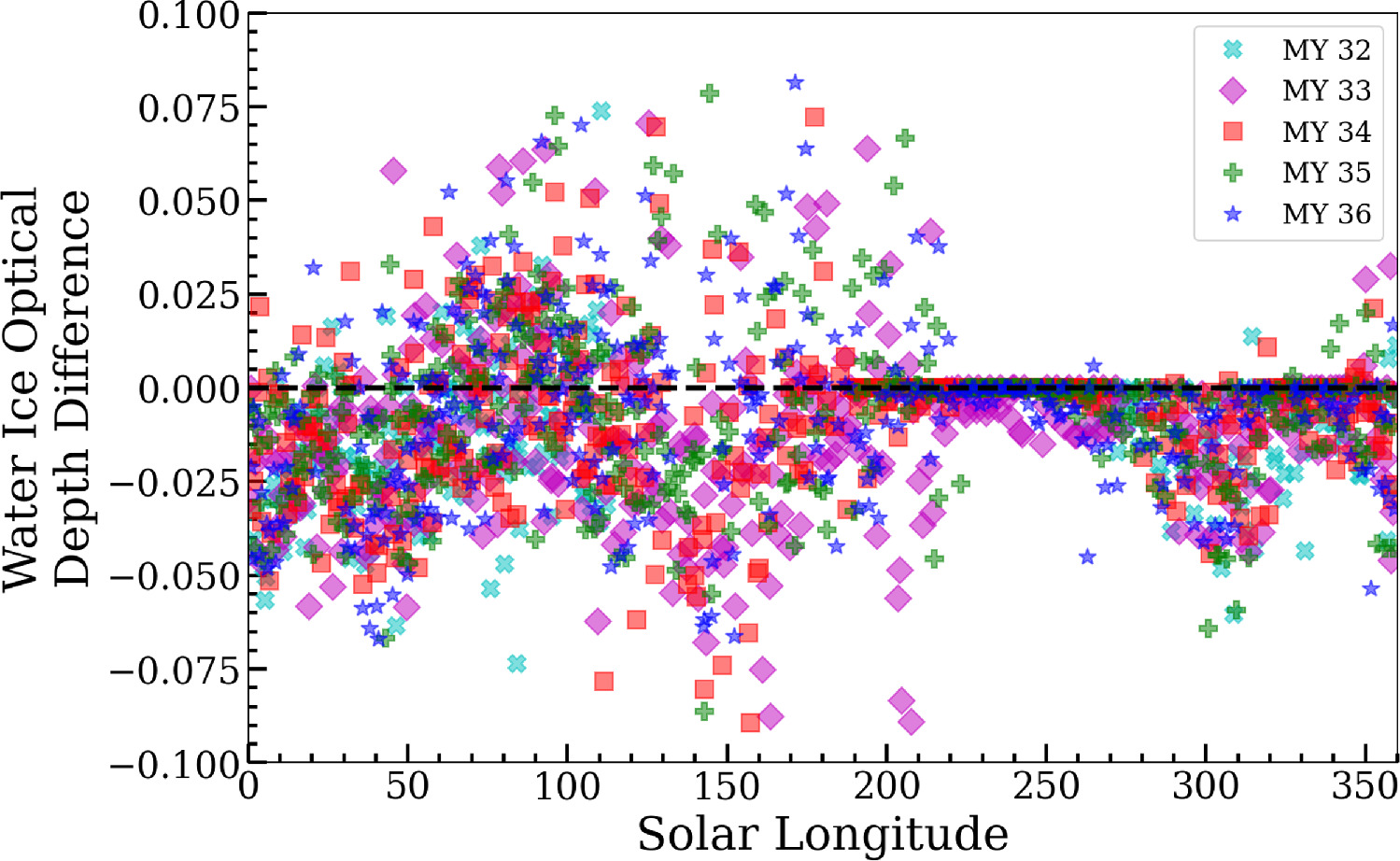
Figure 19. The difference in MARCI water-ice optical depths between the north- and south-facing SHM FOVs over MYs 32–36. Outside of the ACB, the south-facing average is almost always greater than the north-facing average, possibly suggesting that the dune fields filling the southern half of Gale are artificially driving up the orbital retrievals. During the ACB, we see higher optical depths to both the north and south, though the south-facing retrievals are, on average, higher than those to the north.
Download figure:
Standard image High-resolution imageBecause our cloud movies point southward during the ACB season, it is important to keep in mind that this surface reflectance effect may be leading to an imperfect comparison between the ground-based and orbital optical depth retrievals. However, if the orbital measurements are indeed too high during the ACB season, we can account for this by increasing the value of our phase function normalization, which will lower the optical depth values to match without affecting the overall fit.
4.4. Comparison with Other Phase Functions
Determining the shape of the scattering phase function is useful not just for our opacity calculations. Because the shape is a consequence of the microphysical properties of the cloud scattering centers, it can reveal details about the physical nature of the ice crystals that make up the cloud. This is of critical importance to the development of Martian global climate models, which generally assume the presence of spherical ice crystals.
Cooper et al. (2019) compared the results of the MSL PFSS observation to analytically derived phase functions for seven randomly oriented ice crystal geometries frequently found in terrestrial cirrus clouds (Yang & Liou 1996; Yang et al. 2010). Based on the results of their analysis, they concluded that ACB clouds are unlikely to consist solely of any of the seven geometries investigated. Instead, their derived phase functions could be the result of a mix of ice crystal geometries or an exotic geometry not seen on Earth.
However, these terrestrial data sets do have one serious problem that may limit the validity of their comparison—they were computed for particle sizes of ∼50 μm. Although this particle size is appropriate for terrestrial applications, it is approximately 1 order of magnitude larger than the particle sizes that have been previously determined for the ACB (3–4 μm; Clancy et al. 2003). This difference is problematic because at the wavelengths to which MSL's Navcams are sensitive, it takes us from a regime where geometric refraction of light through the ice crystals is appropriate to one where Mie scattering must be used. The switch from geometric refraction to Mie scattering will have major consequences for the shape of the phase function, most notably suppressing the peaks at 22° and 46° that are responsible for the wide variety of optical scattering phenomena (e.g., halos and parhelia) that are observed frequently on Earth but have only been conclusively seen once on Mars (Lemmon et al. 2022).
We made use of a database of analytically derived phase functions covering a spectral range of 0.2–100 μm for 189 particle sizes between 2 and 104 μm (Ping et al. 2013; Yang et al. 2013; Bi & Yang 2017). This database includes nine different ice crystal geometries (droxtals, hollow and solid bullet rosettes, plates, single columns, and aggregates consisting of five plates, ten plates, and eight columns) with three different surface roughness conditions (smooth, moderately roughened, and severely roughened). This database allowed us to more realistically approximate what MSL's Navcams would observe by averaging across multiple wavelengths and particle sizes.
To construct our phase functions for each geometry/roughness combination, we averaged together the relevant phase functions for all wavelengths within the Navcam bandpass and particle sizes of 1, 3, and 6 μm. The contribution of each phase function to the final curve is weighted by the relative responsivity of the Navcams at that wavelength. We found that after averaging over the Navcam bandpass, the surface roughness has little to no effect on the shape of the phase function at these particle sizes. Consequently, all figures here were generated using just the smooth geometries (no surface roughness).
For each geometry, the phase functions must be normalized for the results to be meaningful. Ordinarily, phase functions are normalized to either 1 or 4π over scattering angles between 0° and 180°. Since our derived phase functions do not cover this entire range, we instead normalized our phase functions by the median value of the comparison phase function. This normalization procedure was applied to all comparisons.
The ice crystal geometry comparisons are presented in Figure 20. At these particle sizes, the averaging process removes many of the identifiable features in the individual phase functions, leaving us with smooth, generally featureless curves. Because our derived phase functions are also fairly smooth and featureless, it is challenging to say whether or not we should prefer any one geometry over any other. Additionally, none of the comparison phase functions show the "flattening out" behavior that we observe for scattering angles greater than 60°. This difference may suggest that ACB clouds are not composed of nearly pure water-ice crystals but rather something with radically different light-scattering properties, like ice-rimed dust particles.
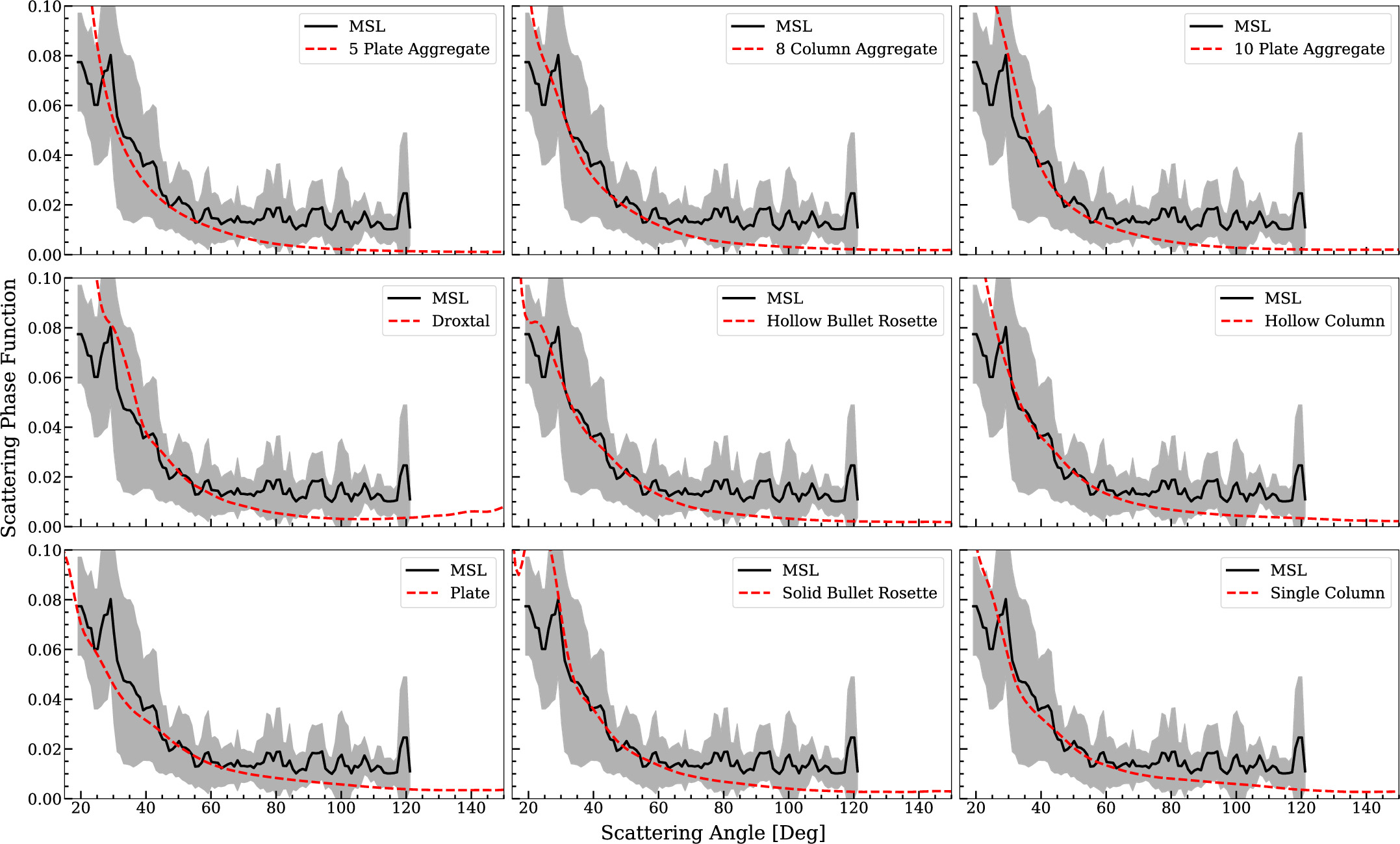
Figure 20. Our derived phase functions compared to the phase functions of nine water-ice crystal geometries frequently observed in terrestrial cirrus clouds, with appropriately Mars-like particle sizes.
Download figure:
Standard image High-resolution imageWe also made comparisons with other phase functions that have been derived for Martian clouds. These included water-ice cloud phase functions from Viking (Clancy & Lee 1991) and the Thermal Emission Spectrometer (TES) on board MGS (Clancy et al. 2003), as well as Viking dust phase functions (Clancy & Lee 1991). The six comparison phase functions are plotted against our MSL-derived phase functions in Figure 21, with the same normalization procedure applied as in Figure 20.
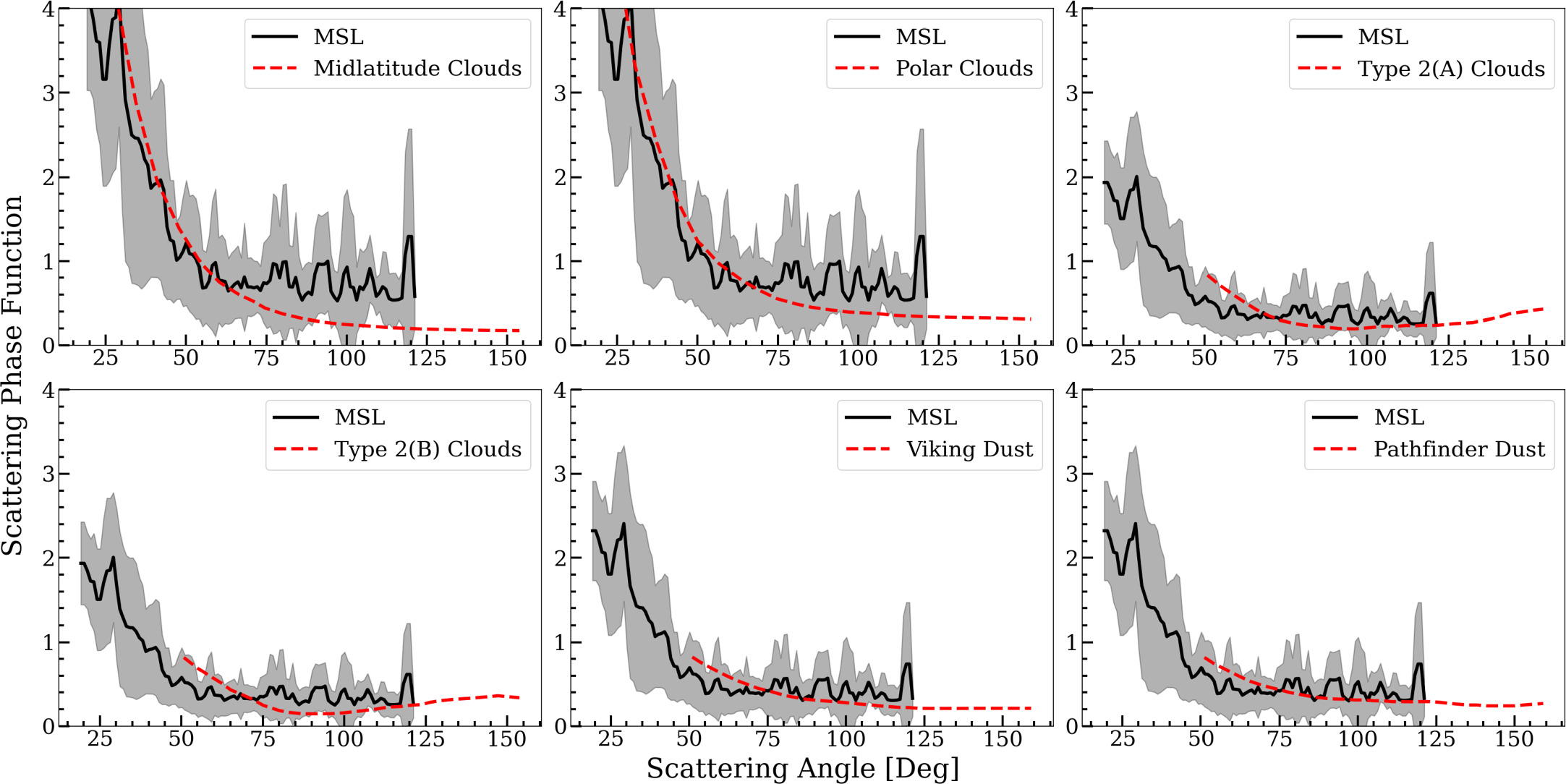
Figure 21. Comparisons between our three phase functions and those previously derived for six cloud types observed on Mars. We can see reasonable agreement between the reference phase functions and those that we have derived, though the limited scattering angle coverage (particularly in the forward-scattering direction) and lack of distinctive features in any of the phase functions make direct comparisons challenging. The different appearance of our phase function in the panels is a consequence of the normalization procedure performed for each comparison phase function.
Download figure:
Standard image High-resolution image
Figure 22. The six PFSS phase functions compared to our derived phase functions (in black with associated 95% confidence intervals) for MYs 34–36. MSL-derived PFSS phase functions agree reasonably well with ours, with the MCS-derived PFSS phase functions agreeing less well with the forward-scattering peak starting approximately 20° earlier. A robust comparison between the phase functions is limited due to the overlap being constrained to the lowest-information portion of the curves.
Download figure:
Standard image High-resolution image
Because we are observing aphelion clouds, we would expect to see the closest agreement with the TES type 2(A) and 2(B) aphelion clouds. Indeed, we can see reasonably good agreement, though the limited range of the TES phase functions makes a robust assessment of the fit challenging. It should also be noted that TES phase functions were derived from observations made in the thermal infrared, while MSL's Navcams operate in the visible. It is known that the optical properties of terrestrial cirrus clouds are quite different in the infrared versus the visible—for example, they are optically thin in the visible but comparatively optically thick in the infrared, leading to their being the only cloud type that creates a net warming effect on Earth's surface (Stephens & Webster 1981). As such, a comparison between the MSL and TES phase functions may not be one-to-one.
The midlatitude and polar cloud phase functions do also appear to follow our derived phase functions relatively closely, though, as with the ice crystal phase functions, they do not level off at large scattering angles in the same way that ours do. Once again, the fact that all of the phase functions are fairly smooth makes a meaningful comparison difficult as they lack specific, distinctive features whose presence or absence could be used as a point of reference.
Additionally, we compared with the phase functions from the PFSS that is also executed as part of the MSL cloud observation campaign. The PFSS consists of nine three-frame movies that form a dome around the rover, covering nearly the entire sky, with the exception of the region surrounding the Sun. A phase function is derived from this observation using Equation (3), so it faces the same question we did in determining which cloud opacities to use as an input. Ultimately, Innanen et al. (2024) opted to derive six phase functions for MYs 34–36: three using the opacities presented herein and an additional three using MCS opacities. The comparison between the PFSS and our derived phase functions for each year is presented in Figure 22.
We would expect to see a close agreement between our phase functions and those derived from the PFSS, as both were constructed from observations of the same clouds at the same location using the same instrument on board the same spacecraft, unlike the Viking and TES phase functions. Indeed, we do see generally good agreement between our phase functions and those derived from the PFSS using MSL opacities. The MCS/PFSS phase functions do not fit as well, as the forward-scattering peak begins about 20° further from the Sun. We previously noted the temporal and spatial resolution challenges of MCS data, which may be responsible for the difference.
In both cases, we cannot evaluate the fit over the full range of scattering angles. Due to its design, the PFSS can observe closer to the backward-scattering direction than the ZMs and SHMs do, but it also cannot observe the forward-scattering peak. Although the PFSS can, in principle, look as close as ∼20° from the Sun, the fact that each pointing uses only three frames (as opposed to the eight used by the ZMs and SHMs) means that in the 20°–40° range, the background signal from the sky becomes increasingly dominant over that from the clouds. This makes it more challenging to robustly extract the clouds from the sky using MFS, adding enough noise to the derived values that they are excluded from the final phase function. By stacking more images to create the mean frame in the ZMs and SHMs, we are able to improve the S/N of the observation, resulting in a more physically plausible phase function at low scattering angles.
5. Conclusions
We have updated the record of water-ice cloud opacities over Gale Crater to cover the first five MYs of the MSL mission (Ls = 160° of MY 31 through Ls = 160° of MY 36). The record now includes five appearances of the ACB, four of which have nearly full diurnal coverage.
For the MY 34–36 ACB seasons, we derived scattering phase functions assuming that the opacities measured at scattering angles >70° were representative of the opacities at all scattering angles. Our phase functions for the three MYs cover a range of scattering angles spanning approximately 130°, from a minimum of 15° to a maximum of 145°. Very little diurnal or interannual variability was seen in the shape of the phase function, consistent with other phase function measurements conducted using MSL data (Cooper et al. 2019; Innanen et al. 2024).
For each MY, we normalize the phase function and compare it to analytically derived phase functions for nine ice crystal geometries (Ping et al. 2013; Yang et al. 2013; Bi & Yang 2017). These reference phase functions are averaged across both particle size and wavelength to replicate the expected size distribution across the Navcam bandpass. We find that the wavelength averaging at these particle sizes suppresses nearly all identifying features for these geometries, making it extremely challenging to compare our phase functions with those from the database. The flattening of our derived phase functions at scattering angles greater than 60° stands out as potentially unusual, as none of the nine comparison phase functions show this behavior. However, previously derived phase functions for ACB clouds (Clancy et al. 2003) are relatively flat at these scattering angles.
After applying the phase function correction to our opacity measurements, we found that the opacity of ACB clouds is remarkably stable, varying very little diurnally, intraseasonally, or interannually. We confirmed that this stability is not a consequence of the assumptions we made to derive the phase functions by artificially restricting the data to just those observations made >70° from the Sun and removing the correction. No evidence for significant variability is seen in the restricted data set either. Although higher-opacity clouds do occur more frequently in the morning, particularly in MYs 32 and 33, morning clouds do not appear to be systematically higher-opacity than those in the afternoon.
Previous work examining the first ACB season with full diurnal coverage (MY 33) reported a 57% difference in the mean opacity of ACB clouds in the morning versus those in the afternoon, with morning clouds being more optically thick than afternoon clouds (Kloos et al. 2018). This difference does not appear in any of the three following MYs, where morning and afternoon ACB clouds have comparable opacities. After applying our new phase functions to the Kloos et al. (2018) data, the reported diurnal variability fails to appear, suggesting that it arose from the application of a flat phase function over a range of scattering angles where such an assumption is inappropriate.
To validate our results, we compare them to opacity retrievals from MARCI on board the MRO and from the EXI on board the EMM's Hope orbiter. We find that our retrievals generally match well with the orbital data with occasional deviations near the beginning and end of the ACB season, potentially indicating the presence of increased atmospheric dust at these times. We also find that neither of these data sets may be appropriate for examining water-ice opacities at the scales observed by MSL. The low resolution of their surface reflectance correction maps creates unusually high-opacity values over the floor of Gale due to the presence of sand deposits that are more reflective in the UV than the average Martian surface.
The study period includes the MY 34 global dust storm (GDS), which occurred between the MY 34 and MY 35 ACB seasons. GDS events have been documented as one of the few phenomena that can disrupt the observed low interannual variability of the ACB. That does not appear to have occurred here, as the MY 34 and MY 35 ACBs are nearly identical, at least when comparing the opacities and the scattering phase function of their clouds. Notably, the MY 34 GDS took place very early in the dusty perihelion season, potentially giving its lasting atmospheric effects more time to return to baseline before the onset of the MY 35 ACB.
Acknowledgments
We would like to thank the MSL science and operations teams for their time and expertise in assembling this data set over the last 10 (Earth) yr, as well as the two reviewers whose comments greatly improved the manuscript. This research was funded in part by the Canadian Space Agency's MSL Participating Scientist program based on a NASA MSL PSP selection, as well as the Natural Sciences and Engineering Research Council of Canada (NSERC) Technologies for Exo-Planetary Science (TEPS) Collaborative Research and Training Experience (CREATE) program.