A historical contingency hypothesis for population ecology

Introduction

The broad role of historical contingencies and laws of nature for explaining natural phenomena has been debated, largely as a matter of metaphysics, for millennia (Harrison, 2016). Laws of nature are theory-based rules that predict the behavior of natural phenomena under an idealized set of conditions, such as Galileo’s law of constant acceleration or Kepler’s law of planetary motion. In ecology, contemporary perspectives on laws of nature include arguments for the existence of a few laws, such as species-area curves and exponential growth (Turchin, 2001; Berryman, 2003; Colyvan and Ginzburg, 2003). When natural phenomena do not behave as predicted by a law, such exceptions are conventionally taken as evidence that some idealized condition of the law has been violated. It is widely appreciated that the ideal conditions required by laws will rarely hold in the real-world, which led to the development of less restrictive, law-like, theory-based explanations – which are typically represented by statistical models and are ubiquitous in ecology. The epistemic value of these laws and theory-based explanations is that they guide the search for explanations to apparent violations and serve as null hypotheses to which real-world phenomena can be compared.

By contrast, natural phenomena can also be explained by historical contingencies, whereby a phenomenon’s behavior is fundamentally determined by the particular order and timing of certain key events in the past. An archetypal example of a historically contingent event for the natural sciences is when an asteroid collided with Earth 66 million years ago and fundamentally altered patterns of species diversity and vertebrate evolution. Law- and theory-based explanations of nature differ importantly from explanations based on historical contingencies inasmuch as the former are typically expressed in mathematical terms which readily allows for a quantitative evaluation of their explanatory power. Moreover, while assessments of the importance of historically contingencies are rare in ecology, substantial effort is spent searching for regular patterns, or theory-based explanations that might hint at laws of nature. The motivation for that substantial effort is a belief that finding law-like explanations will improve the accuracy of predictions or forecasting future dynamics. Contemporary perspectives on historical contingency exist for a few phenomenon in ecology and evolution, such as adaptive radiation and the assembly of ecological communities (Losos, 1994, 2010; Fukami, 2015). In community ecology, a conceptualization for historical contingency focuses on contingency as an emergent property of ecosystems and how the functional role of a species is frequently contingent on the biotic and abiotic conditions of the ecosystem (Schoener, 1986; Simberloff, 2004; Schmitz, 2010). Another conceptualization states that (Lawton, 1999): “Contingent means ‘only true under particular or stated circumstances’. A contingent rule (or law) takes the form: if A and B hold, then X will happen, but if C and D hold, then Y will be the outcome. It follows that patterns will also be contingent and so will theory. Some of the contingency may be ‘historical accident’ in its broadest sense, from the impact of meteorites to the vagaries of chance mutations…” That conceptualization seems to posit historical contingencies as secondary variables or factors which cause natural phenomena to deviate from the behavior predicted by laws of nature, rather than being a process with significant explanatory value in its own right. These conceptualizations have likely contributed to a belief that historical contingencies cannot be useful as general explanations because historically contingent events and their effects are too specific to each case (Fukami, 2015; Harrison, 2016). One response to that concern is that (Simberloff, 2004): “because communities are idiosyncratic, elucidating their structure and workings should be aimed not at deducing general laws but rather at amassing a catalog of case studies (Shrader-Frechette and McCoy 1993). These case studies serve two main purposes. [First] Individually, they can help to solve specific environmental problems.... Second, as a group, case studies can point to rough generalizations that can … advance both theory and practice.” However, none of these conceptualizations of historical contingency are expressed in a way that readily allows for the explanatory power of historical contingencies to be assessed and quantified.

The historical contingency hypothesis

In this study, we evaluate historical contingencies as a general explanation for phenomenon in population ecology. We do so through the development of a historical contingency hypothesis (HCH) and a simple framework that allows for the explanatory power of historical contingencies to be quantified and compared to other kinds of scientific explanation, especially statistical models associated with either the assessment of underlying mechanisms or forecasting. We also highlight how the HCH helps explain several basic phenomena in population ecology, namely the commonness of ecological surprises (Doak et al., 2008) and ecologists’ limited capacity for forecasting future dynamics (Beckage et al., 2011; Yates et al., 2018).

The essence of the HCH for populations is that population-level phenomena are well explained as being the result of a series of historically contingent events. That is, a series of random events characterized by (1) significant legacy effects that are comparable in length to the waiting time between such events, and (2) the disparate nature of individual events in the series. For example, one event might be a novel disease, the next a severe weather event, and the next a disturbance, such as a forest fire. The effect of each of these events persist long after the events have occurred, and in this sense the events have legacy effects (Moorhead et al., 1999; Cuddington, 2011). Populations are constantly exposed to all manner of random events – most of which are insignificant. What distinguishes historically contingent events from other random events is that they have both important and long-lasting legacy effects. Furthermore, although some events may be extreme, others may be the coincidence of several common events that have synergistic effects (Denny et al., 2009). Although a historically contingent event would tend to be identified after its occurrence, that circumstance does not make historically contingent events ad hoc or arbitrary explanations. The explanations are not ad hoc or arbitrary to the extent that the event in question can reasonably be called a cause of the dynamics that followed.

The HCH is also usefully understood as a synthesis of several important concepts in population ecology. In particular, some historically contingent events may be classified as tipping points or ecological surprises that result in alternate stable states. Some historically contingent events may also be classified as a large pulse disturbance or a press disturbance whose effects last for some time [sensu, Figure 1 of (Inamine et al., 2022)]. Others have shown those concepts to be important (Bender et al., 1984; Beisner et al., 2003; Doak et al., 2008; Holt, 2008; Scheffer et al., 2009; Selkoe et al., 2015). However, the HCH goes beyond those concepts, in part, by supposing that the events of the HCH occur frequently enough within a single system to represent an essential explanation for that system’s dynamics over longer periods of time. For example, detection of a single tipping point or a single switch from one stable state to another would seem insufficient to conclude that a population’s dynamics are broadly characterized by the HCH. The insufficiency would be associated with not knowing (1) how long the population had been in its prior state or will be in its current state or (2) enough about the diversity of events that cause switches within a system. The greater the diversity of events in the series, the more difficult it would be to predict the next event, because the next event may be of a kind that hasn’t been previously observed.

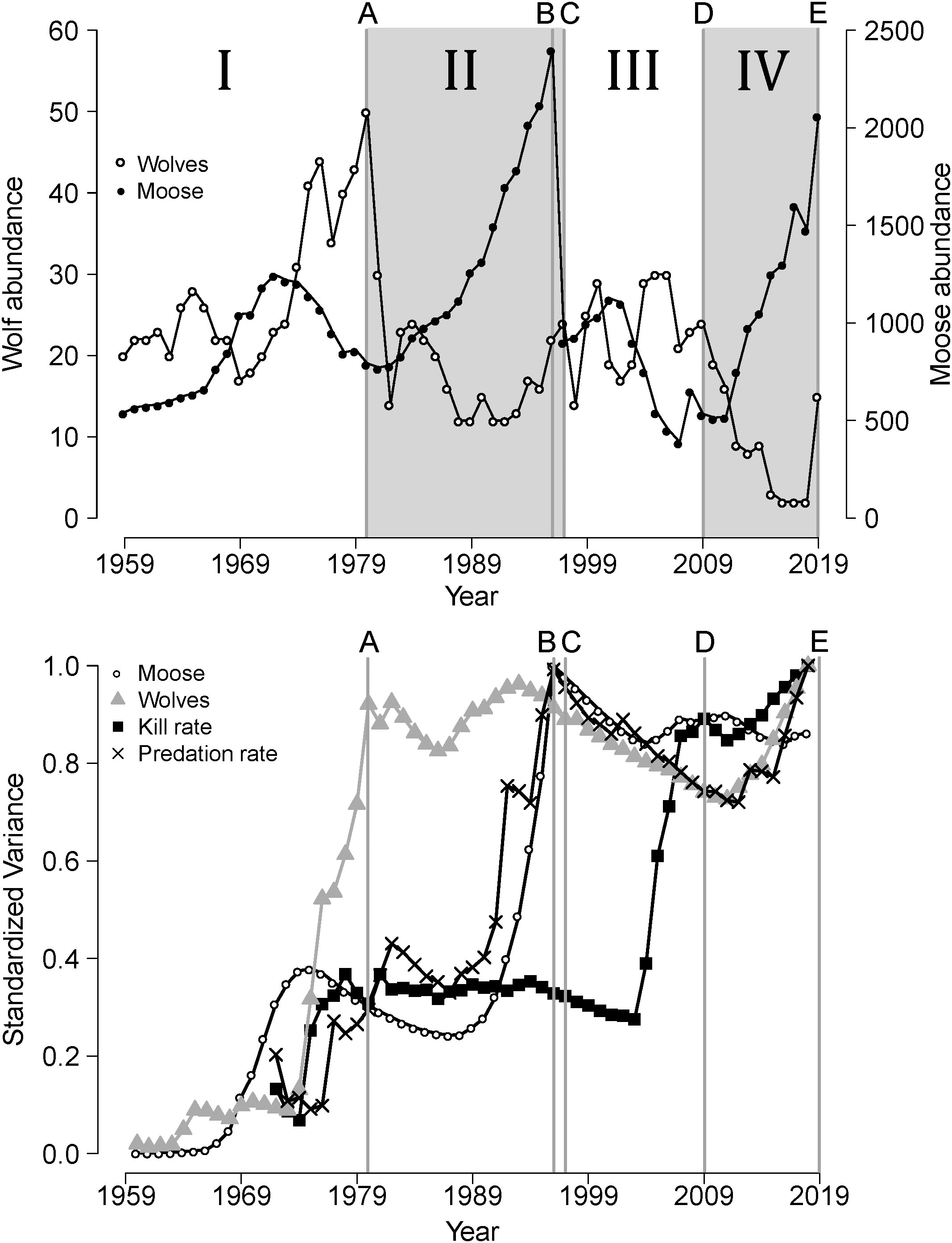
Figure 1 The upper panel depicts abundances of wolves and moose in Isle Royale National Park (1959-2019), divided into four periods (I, II, III, IV) demarcated by events A-E. The nature of each event is described in the Study System. The lower panel depicts cumulative variances (scaled to one) of time series representing essential elements of predator-prey dynamics on Isle Royale.

The HCH is categorically distinct from conventional forms of environmental stochasticity (Lindstrom et al., 1999). Traditional models of environmental stochasticity focus on processes that occur every year, whose influence in any given year could be extreme, nil, or anywhere in between, and whose influence is characterized by the phenomena’s variance, skew, and kurtosis. Environmental stochasticity may be used to represent a single process, such as precipitation, or it may represent the sum of many exogenous processes that occur every year and then registered as an adjustment to, for example, some vital rate. Furthermore, legacy effects are not of explicit interest of most models of environmental stochasticity. By contrast, historical contingency involves relatively infrequent events (e.g., occurring once every 1-2 decades or 3-4 generations) with long-lasting legacy effects. As such, one wouldn’t expect a population’s dynamics to be explained by the HCH if it had been monitored for only a short time.

With the preceding conceptualization, we develop a pair of quantifiable hypotheses which represent strong and weak versions of the historical contingency hypothesis (HCH). The strong HCH is that a population’s ecology is fundamentally driven by historically contingent events. The strong HCH would be supported if models that explicitly account for historically contingent events explain a substantial portion of a phenomenon’s past dynamics. The weak HCH is that historical contingencies have an important modifying influence on a population’s ecology by altering a population’s underlying ecological relationships. For example, when a population is governed by the weak HCH one expects the fit of a theory-based model of ecological relationship to be improved by modifying it to explicitly account for historically contingent events. An important distinction between the two versions of the HCH is that the strong version assesses historical contingencies as an essential basis of explanation in its own right. By contrast, the weak HCH is more closely related – though not identical – to earlier conceptualizations of historical contingencies, which suggest that historical contingencies are secondary variables or factors (e.g., Lawton, 1999).

The aim of this study is to assess the extent to which the HCH can explain phenomena in population ecology. In doing so – we note here and further explain below – how the standards for assessing the explanatory power of a model depends on whether the model’s purpose is to make a forecast, opposed to assessing some particular mechanism. We fulfil the aim of this study by evaluating the extent that HCH models explain the population ecology of the wolf and moose system in Isle Royale National Park using data collected over a 48-year period (1971-2018). Specifically, we evaluate the extent that HCH models explain predation rate, which is the portion of the prey population killed by predation per unit time. We focus on predation rate (PR) because it is a synthesis of the three most basic elements of a predator-prey system, i.e., predator abundance, prey abundance, and kill rate, which is the process that connects the abundance of predator and prey. More specifically, predation rate (PR) is calculated as per capita kill rate (KR), times predator abundance (P), divided by prey abundance (N).

Reddened spectra

Ecological time series whose process variance tends to increase with increasing periods of observation are said to have reddened spectra (Ariño and Pimm, 1995). Reddened spectra are common among populations that have been observed for long periods of time (Inchausti and Halley, 2001, 2002) and the presence of reddened spectra is associated with an increased difficulty of predicting future dynamics, including the estimation of extinction risk (Lawton 1988). However, the processes that lead to ecological time series exhibiting reddened spectra are not well-understood (Akçakaya et al., 2003). Some have reasoned that reddened spectra may be the result of populations experiencing a series of tipping points, alternative stable states, and ecological surprises (Poole, 1978; Ariño and Pimm, 1995). That reasoning is supported, in part, by simulation studies which have shown shifts in stable states may be preceded by punctuated increases in variance (Carpenter and Brock, 2006). If reddened spectra are typically associated with those processes, then it is at least plausible that the HCH is broadly significant. In this paper, we provide a partial assessment of these ideas by assessing whether the timing of historically contingent events in the Isle Royale system correspond to the emergence of reddened spectra.

Study system

Isle Royale (544 km²) is an archipelago located in Lake Superior, North America (47°50′N, 89°00′W) approximately 24 km from the mainland. Isle Royale is a National Park and a legally-designated wilderness area and neither the wolves, moose, nor the forest, have been harvested for almost a century. The wolf-moose system has been influenced by a series of disparate random events over the last 50 years (denoted A through E in the upper panel of Figure 1). Event (A) was the outbreak of a novel disease that occurred in the early 1980s and impacted the wolf population. Specifically, canine parvovirus was inadvertently brought to Isle Royale by humans shortly after it evolved into existence in the late 1970s (Peterson et al., 1998). That disease outbreak coincided with the highest density of wolves ever observed and represents a time of intense intraspecific competition for prey. Event (A) was followed by a crash (~70% decline) in the wolf population (Figure 1, upper panel).

Event (B) occurred in 1996 and was the most severe winter ever recorded in the Lake Superior region. The severity of that winter is indicated by record-breaking temperatures and snow depths (Peterson, 1996). For example, snow was the deepest ever recorded on Isle Royale, being almost twice as deep as the mean snow depth observed over the last 50 years, and deep snow persisted until late April (Peterson, 1996). Deep snow restricts the ability of ungulates to move around and find food and thereby has an important negative impact on their nutritional condition and body mass (Weladji et al., 2002). That severe winter coincided with the highest density of moose ever observed on IRNP (~4.4 moose/km²) and represents intense intraspecific competition for forage. The impact of event (B) was a ~60% decline in moose abundance (Figure 1, upper panel).

Event (C) occurred in 1997, one year after the severe winter, when a wolf emigrated from the mainland to the island by crossing an ice bridge. (Ice bridges form only occasionally and wolves cannot survive the 24 km swim to Isle Royale.) Event (C) changed a long-held assumption that there was no gene flow into the island’s wolf population, and no naturally occurring gene flow has been detected since event (C). The immigrant wolf represented a genetic rescue event, whose effects were so profound they are best described as a genomic sweep (Hedrick et al., 2014). That genomic sweep was indicated by a rapid spread of the immigrants genes among the population, such that within a decade, approximately 60% of the genes in the wolf population’s had been inherited from the immigrant [see Figure 2 in (Hedrick et al., 2014)]. That genomic sweep was associated with important increases in the fitness of the wolf population (Hoy et al., 2023), which had been suffering from severe inbreeding depression just prior to the immigrant’s arrival (Hedrick et al., 2014).

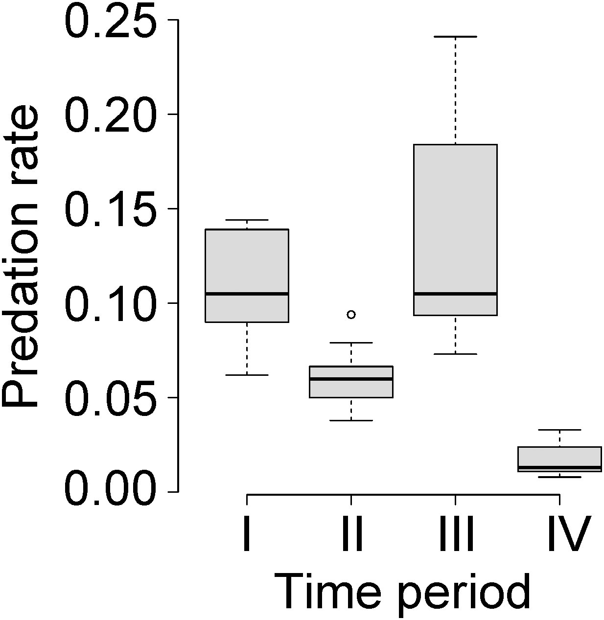
Figure 2 Box-and-whisker plot for predation rate by wolves on moose in Isle Royale National Park for each time period demarcated by the historically contingent events described in the Study System and depicted in Figure 1. More precisely, the cut-offs used for each time period are the same as those used in Model 3 in Table 1. Thick black lines represent the median values and grey boxes are interquartile ranges.

Event (D) is the reappearance of canine parvovirus between 2007-2009, after a 17-year (4 generation) absence which coincided with the resumption of severe inbreeding depression and the end of the benefits of the genetic rescue (Vucetich and Peterson, 2008; Peterson and Vucetich, 2014). More precisely, the beneficial influence of genetic rescue on the wolf’ population’s fitness waned throughout the period 2008-2010, when the immigrant’s ancestry began to decline (Hedrick et al., 2014). The resurgence of inbreeding depression that followed event (D) resulted in the wolf population collapsing to two wolves, a father-daughter pair that were also half siblings (Hedrick et al., 2017). Unsurprisingly, these highly inbred wolves never produced offspring that survived to adulthood. As the wolf population headed towards extinction, the moose population more than tripled and the concomitant increase in moose browsing had a severe impact on forest vegetation in large areas of Isle Royale (Hoy et al., 2019). Those circumstances led the National Park Service (NPS) to translocate 19 wolves to Isle Royale (from other populations in the Lake Superior region) between autumn 2018 and autumn of 2019 to restore the wolf population (Hoy et al., 2019). This anthropogenic intervention (event E) was surprising, because traditional NPS policy, and the majority of the decision-making process, pointed toward the NPS not intervening (Vucetich, 2021).

These events (A-E) were not only unexpected, but they also had important long-lasting legacies. Specifically, following event (A), the first canine parvovirus outbreak, predator abundance remained low for more than a decade whilst prey abundance rose exponentially which triggered the first trophic cascade ever documented in a terrestrial ecosystem (McLaren and Peterson, 1994). More precisely, event (A) shifted control of prey population dynamics from a top-down processes to abiotic processes for more than a decade (Wilmers et al., 2006). The impact of events (B/C), the severe winter/arrival of an immigrant wolf, was a greatly reduced prey population and predator population with increased fitness, which ushered in a decade-long period of strong top-down influences. Event (D), the second disease outbreak coinciding with the resurgence of inbreeding depression in the wolf population, instigated a prolonged period of negligible top-down processes and the start of another trophic cascade, represented by collapse of the wolf population, exponential rise of the moose population, and severe damage to forest vegetation (Hoy et al., 2019, 2023). Although it is too soon to evaluate the long-term consequences of event (E), the translocation of wolves, early signs indicate that it will leave a significant legacy. For example, the wolf population rose from 2 to 15 wolves between 2018-2019 and exhibited the highest per capita kill rates ever observed in this system (Hoy et al., 2019). Moreover, some of the translocated wolves were significantly larger than the native Isle Royale wolves which can importantly affect predator-prey dynamics (Emmerson and Raffaelli, 2004). These five events represent historically contingent events as conceptualized in the Introduction. They were all recognized as major events in the chronology of wolves and moose upon being observed and long before we formulated the HCH. In other words, these events were not selected in an ad hoc manner for the purpose of building the statistical model described below. Finally, these events divide the chronology of wolves and moose of IRNP into four periods of time (I to IV, see Figure 1, upper panel) that form the basis for developing a quantitative model of the historical contingency hypothesis.

Data & analysis

In this section, we describe the data used to perform our analysis. Next, we describe and assess the statistical models we built to represent the HCH. Then, we compare HCH models to traditional theory-based models whose purpose is to explain underlying mechanisms. Lastly, we also compare the HCH models to alternative models whose purpose is to forecast future dynamics.

Data

We assessed the HCH’s ability to explain predation rate, which is the proportion of the moose population killed by wolves over a 48-year period (1971-2018). The first year of the study period is 1971, because that is the first year that estimates of predation rate are available (see below). The last year of the study period is 2018, because that year marks the end of period IV, when wolves were translocated to Isle Royale. (We did not extend the study period beyond 2018 because insufficient time has passed to assess a fifth time period.)

Predation rate is calculated as the per capita kill rate multiplied by wolf abundance and divided by moose abundance (Vucetich et al., 2011). The three elements of predation rate are estimated independently in this study system each winter (Vucetich et al., 2011). More precisely, wolf and moose abundance have been estimated every year since 1959 and kill rate has been estimated every year since 1971. Moose abundance (N) was estimated annually using a random stratified sampling design and aerial surveys conducted between late January and early February (Peterson and Page, 1993). Wolf abundance (P) was estimated by aerial census from a fixed-wing aircraft in winter (January early March) using methods described in (Vucetich and Peterson, 2004). The per capita kill rate (KR) is the number of moose killed per wolf per time unit (Vucetich et al., 2011). Each winter we observed the number of moose killed by wolves during a period of ∼44 days (mid-January to early March) during aerial surveys in a fixed-wing aircraft (Vucetich et al., 2011). The carcasses of wolf-killed moose were detected by direct observation, by following wolf tracks left in the snow, and by regularly searching areas which packs had visited. We also detected wolf-killed moose while carrying out ground-based field work.

To perform the analyses described below, we also make use of data that include estimates of average pack size for the wolf population (PS) and several weather variables. We calculated PS as the average number of wolves in packs observed during aerial surveys each winter between 1971-2018. The weather variables that we assessed were mean temperature in winter (WT) and mean North Atlantic Oscillation (NAO), which are indicators of winter severity. We also considered mean temperature during the previous summer (ST) because summer temperature is thought to influence the nutritional condition and parasite burdens for moose – factors that may make moose more vulnerable to predators (Hoy et al., 2021, 2022). We obtained station-based measurements of the North Atlantic Oscillation (NAO) index for each winter (January-March) from the National Center for Atmospheric Research (Hurrell, 1995). We obtained estimates of the mean temperatures each winter (January to March) and summer (July to September) from a near-by weather station in northeastern Minnesota, located approximately 40-60km from Isle Royale (Western Regional Climate Center, 2016).

The strong HCH

To test the strong HCH, we built a model to quantify the portion of variation in predation rate that can be explained only by historically contingent events. Specifically, we used a model of predation rate characterized by four intercepts (no slopes), where each intercept represents a different time-period delineated by historically contingent events (Figure 1, upper panel). The first year of period I is 1971 (first year that estimates of predation rate are available), the first year of period II is 1980 (occurrence of event A), the first year of period III is 1997 (occurrence of event B/C). Period III ends and period IV begins with both the reappearance of a disease, the resurgence of severe inbreeding depression and the waning benefits of genetic rescue and is not readily assigned to a single year. As indicated in the Study System section, Period III ends and period IV between 2008 to 2010. Consequently, we built three models of historical contingency, each with a different year starting period IV (i.e., 2009, 2010, and 2011). The last year of period IV is 2018 (occurrence of event E).

The three models of the strong HCH (with different years starting period IV) explained between 53% and 59% (average of 56%) of the variance in predation rate (Table 1; Figure 2). In other words, historically contingent events explain over half of the variance in predation rate. R² values of that size for time series of population-level phenomena are generally considered to represent ecologically significant explanations.

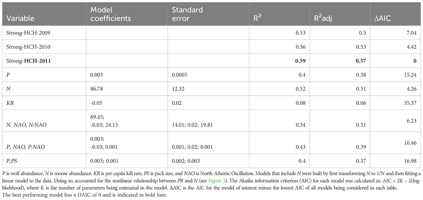
Table 1 Performance of the strong historical contingency hypothesis models and alternative theory-based models built to understand mechanisms underlying interannual variation in predation rate between 1971-2018.

Models for comparison

An important aspect of assessing the HCH is to compare its explanatory power to other forms of scientific explanation, especially theory-based explanations by which we mean statistical models motivated by ecological theories and hypotheses. In this section we explain the merits and limitations of various models to which the HCH model might be compared. Given our interest to explain fluctuations in predation rate, Lotka-Volterra theory and some of its elaborations are an appropriate place to begin. However, before describing the various models that we built for comparison, it is first necessary to discuss two preliminary issues.

Preliminary #1: statistical circularity

As a concept rising from predation theory, PR is defined as KR×P/N. Distinct from its relationship to predation theory, PR is also a statistical variable that we calculated as KR×P/N. This circumstance can lead to a kind of circularity that is not uncommon in efforts to assess theoretical expectation with empirical observation (Ritson and Staley, 2021). Consider, for example, fitting this statistical model to our data:

That statistical model seems worth considering given is similarity to the theoretical definition of PR. Yet, the assessment of this model would offer little insight, because its explanatory power rests largely on a circularity due to the structure of the statistical model being so similar to how PR – the statistical variable – was calculated.

This circularity is largely avoided if one had estimates of PR that are statistically independent of N, P and KR, such as an estimate based on observing the annual rate of predation among a reasonably large sample of individually marked and tracked moose (i.e. individuals fitted with GPS-collars). However, such data do not exist for moose over the 48-year study period examined here. Furthermore, such data are not required to realize the main aim of this study, which is to assess the explanatory power of the HCH, in part, by comparing it to theory-based explanations. This circularity is also avoided if, for example, one considers models of PR that contain only one of these variables, N, P, or KR. We explain how and why in Models Motivated to Assess Mechanism.

Preliminary #2: purpose affects assessment

The assessment of a model depends on the model’s purpose. Two general purposes of a model are reflected by two schools of thought in the philosophy of science, realism and anti-realism (Craig, 1998). The salient features of these schools of thought are:

• Realism supposes that the purpose of a model is to assess an underlying hypothesized mechanism. The idea is familiar to practitioners of ecology: develop a prediction that rises from the hypothesized mechanism and then see if the prediction matches the data. The explanatory power of the model depends on several considerations: (1) how well the data fit the prediction, (2) how compelling the hypothesized mechanism is, and (3) the extent to which alternative mechanisms can result in the same prediction.

• Anti-realism supposes that explanatory power is largely (or entirely) due to a model’s ability to make a parsimonious forecast.

Realism and anti-realism are often viewed as competing ideas, in part, because models that are especially good for one purpose (say assessing mechanism) are often not as good for the other purpose (say forecasting). We do not suppose that either idea or purpose is more important than the other. However, it is important to recognize that an appropriate assessment of a model’s performance depends on its purpose. In the next two sections, we develop a basis for assessing the HCH by comparison to models whose purpose is primarily (1) to assess mechanism or (2) make a parsimonious forecast. We also discuss how the second comparison has value even though the purpose of the HCH is not to make a forecast.

Models motivated to assess mechanisms

Here we consider models that are motivated by the assessment of some underlying mechanism or basic pattern whose importance is indicated by theory, such as the relationship between N and PR. While PR is calculated from N, that relationship still has enough degrees of freedom such that the empirical relationship may be positive or negative, linear or non-linear, monotonic or non-monotonic, strong or weak. No less important, a great deal of meaning has long been attached to knowing the relationship between N and PR (e.g., Holling 1959, Messier 1994, Křivan 2008). The degree to which N and PR are positively related is the degree to which predation has a stabilizing influence on prey density. According to theory, as PR becomes independent of N or increasingly negatively density dependent, then predation becomes an increasingly destabilizing force.

(Note, within frequentist statistics, if a predictor variable and response variable are not statistically independent, then p-values associated with their covariance will be biased. Important as that principle is, it does not undermine the reliable insight that can come from assessing the relationship between N and PR in ways that are not so reliant on the need for unbiased p-values.)

These circumstances about N and PR also apply to the relationship between P and PR and the relationship between KR and PR. That is, there are enough degrees of freedom in either relationship to make their assessment worthwhile and these relationships may be positive or negative, strong or weak, etc. Furthermore, significant meaning has been given to knowing whether and how PR is related to P and KR. For example, the relationship between PR and P is associated with understanding whether and how predation rate is influenced by interference competition among predators (Abrams, 1993). The relationship between KR and PR is associated with, for example, questions about whether “good years” for predators (high kill rate) tend to be bad years for prey (high predation rate, Vucetich et al., 2011).

Based on those considerations about mechanism and process, we compared the HCH model to univariate models that predict PR from KR, P, and N (Table 1). Of those three models, only the model with N performed comparably to the HCH models (e.g. the model with N as a predictor explained 52% of the variation in PR, Figure 3). Many other models can be built with the aim to better understand the mechanisms and processes of predation. We consider three such models. The first two models that we considered are motivated by an interest to assess whether winter severity, a key element of the abiotic environment, has an important influence on PR. We used NAO as an indicator of winter severity, because NAO, a measure of large-scale atmospheric processes, is thought to be a better indicator of overall winter weather conditions than locally measured, singular aspects of weather (i.e., winter temperature).

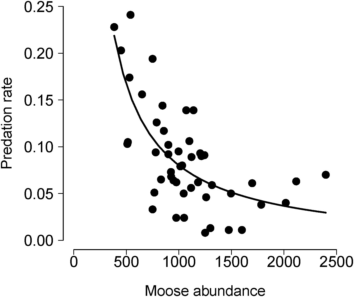
Figure 3 Annual estimates of predation rate (PR) in relation to prey (moose) abundance for the wolf-moose system in Isle Royale National Park. The solid line in depicts fitted values from the univariate model including N in Table 1. Specifically, the line represents PR_predicted = β₀ + β₁(1/N). This model accounts for the non-linearity because PR_observed is calculated as a function of 1/N. That is, PR_observed = KR×P/N. See also Equation 1.

First, we built a model that predicts PR from N and NAO and their interaction. That model represents the hypothesis that the influence of N on PR may also depend on NAO because winter severity may influence how vulnerable moose are to coursing predators, such as wolves. The mechanism for such an influence would be the adverse impact that winter severity tends to have on the mobility or body condition of ungulates (Parker et al., 2009). The second model that we built predicts PR from P and NAO and their interaction. That model represents the hypothesis that the influence of P on PR may also depend on NAO because winter severity may influence a predators’ behavior or ability to detect, encounter and pursue prey (Droghini and Boutin, 2018). Finally, we built a model that predicts PR from P and pack size (PS). This model is motivated by an interest to assess whether the predator population’s social structure has an important influence on PR (Hayes et al., 2000; MacNulty et al., 2012), while also accounting for the influence of P.

The data from Isle Royale provide little or no support for the hypotheses represented by those three models given that none of them performed better than the simpler univariate models nested within each of those three multivariate models. Specifically, the p-values for likelihood ratio tests comparing each of the three models to a nested univariate model (with N or P) were all greater than 0.26. Moreover, the p-values for the coefficients associated with NAO, PS and the interaction terms were all greater than 0.12. Additionally, none of those models performed better than the HCH models in terms of AIC. However, the level of support these three models offer for their respective hypotheses does not depend on each of these models having the highest R² or lowest AIC. Although, many other models could be assessed – each motivated by an interest to assess some reasonably considered mechanism – doing so is likely to result in data dredging, which greatly risks confusing “The best model” with an overparameterized model with an inflated measure of model fit and underestimated p-values.

Models motivated to explain via forecasting

In some scientific contexts, the capacity to explain phenomena is judged by a model’s capacity to make an accurate forecast. An appropriate method for forecasting is cross-validation, which is valuable for avoiding models with inflated measures of model fit and underestimated p-values. Cross-validation may be conducted by any of several different methods. The most appropriate method depends on the purpose and context of the analysis. In our case, the data are relatively limited, compared to the number of potential predictors (n = 48 years) and the purpose is to understand the extent to which a model built over one period of time can predict dynamics over a subsequent period of time. For these reasons, we used the first 24 years of the study period (1971-1994) as the training dataset and used the last 24 years of the study period (1995-2018) as the testing dataset. To find a parsimonious model with the test data, we used AIC and a forward-stepwise-selection procedure with five candidate predictor variables (N, P, KR, PS, NAO). To avoid statistical circularity (discussed above), we did not consider any model that contained all three of the variables used to calculate predation rate (N, P and KR). After finding the most parsimonious model, we used the coefficients (slope and intercept) from that model to generate predictions of predation rate for the test dataset. Then we used R² to judge how well that model predicted predation rate for the test dataset (1995-2018).

The most parsimonious model identified for the training dataset was a bivariate model with P and KR as predictors which explained 80% of the variation in PR between 1971-1994 (see filled circles in Figure 4). However, that model was a poor predictor of predation rate for the test dataset (1995-2018) as it explained only 13% of the variance in PR (see open circles in Figure 4). A conclusion to draw from this analysis is: while PR may be influenced by P and KR, they do not – by themselves – represent a very satisfying explanation of interannual fluctuation in PR, and they do not seem to be a better explanation than the HCH models.

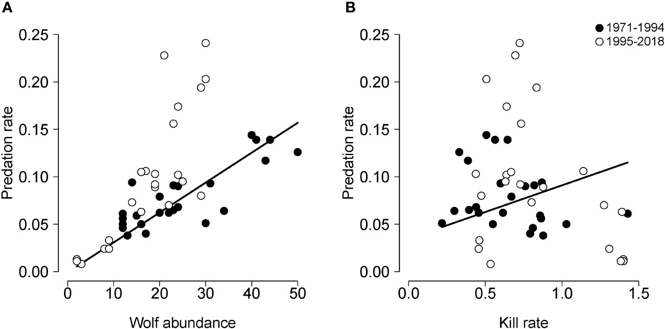
Figure 4 Results of cross-validation for a model forecasting predation rate (PR) as a function of: (A) wolf abundance and (B) the per capita kill rate. Filled circles indicate the training dataset, i.e., data collected during the first 24 years of the study period (1971-1994). Open circles indicate the testing dataset, i.e., data collected during the last 24 years of the study period (1995-2018). The solid line indicates predicted values of predation rate for the testing dataset.

Models motivated to explain via hindcasting

Models designed to explain phenomena via forecasting demand more data than is commonly available. That circumstance leads many to search for explanations of ecological phenomena by hindcasting, even though that approach routinely involves data dredging, often through the use of automated procedures. Because that approach is common, we also consider it as a basis for generating models to compare with the HCH model.

For this assessment, we considered the same five variables that we considered in the forecasting analysis (N, P, KR, PS, NAO), plus two additional weather variables, i.e., average temperature in winter (WT) and summer (ST). We considered winter temperature as an alternative indicator of winter severity. We considered temperatures during the previous summer (ST) because summer temperature is thought to influence the nutritional condition and parasite burdens for moose in winter, which may make moose more vulnerable to predators (Hoy et al., 2021, 2022). The goal of this analysis was to build many models to find the model with the highest R² and lowest AIC – but still avoid the circular model (including N, P, and KR). We began by building each univariate model and each bivariate model. Then we modified the best bivariate model (which included N and P) by sequentially adding variables from the remaining set of candidate variables to see if it improved model performance.

This procedure resulted in 32 models (Table 2). The best univariate model included N (explaining 52% of the variance), and the best bivariate model included N and P (explaining 72% of the variance). The model with lowest AIC and highest R² included three variables, N, P and NAO; however, that model did not perform substantially better than the best bivariate model (ΔAIC = 0.65). Importantly, there is a high degree of statistical dependence between the response and predictor variables contained in the best hindcasting models because they contain two of the three variables used to calculate PR (N and P). Of the models that did not contain a high degree of statistical dependence, the best performing model included two predictors, N and PS. That model explained 64% of the variation in PR, which is slightly higher than the best HCH model (which explains 59% of variance). We suspect that the good performance of the model including N and PS is importantly attributable to PS being very strongly correlated with P (r = 0.81), as opposed to pack size being an important explanation of interannual fluctuations in PR.

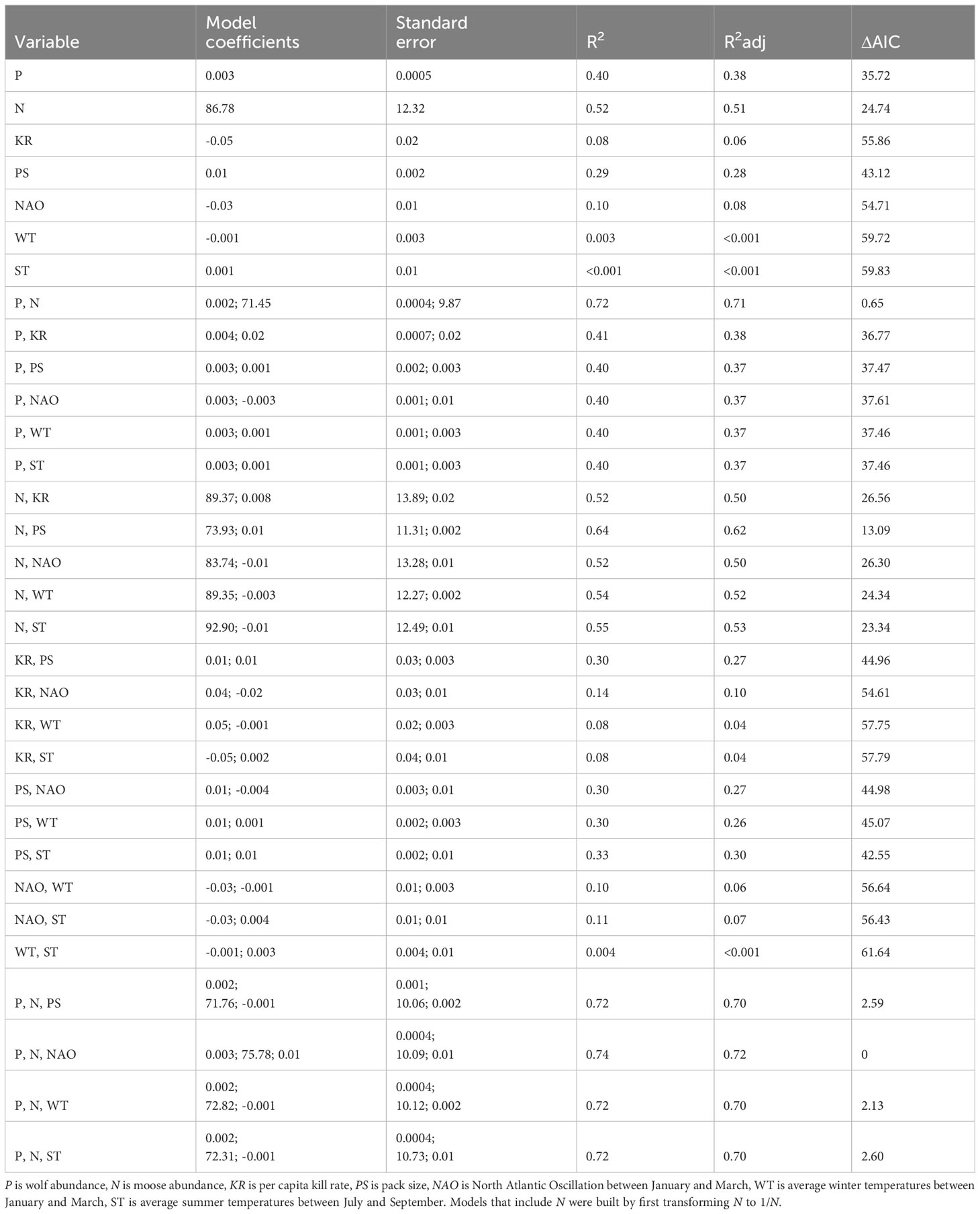
Table 2 Performance of models built to hindcast interannual variation in predation rate between 1971-2018.

Ratio-dependent models

The preceding sections distinguished models on the basis of their purpose – mechanistic assessment or parsimonious prediction. Some models are not so simply categorized. An example of such is a ratio-dependent model, which predicts KR from N/P or P/N. Ratio-dependent models are not so simply categorized because researchers disagree on the epistemic value of these models. Some think this model is an especially parsimonious representation of an important mechanism, i.e., the separate influence of N and P on KR (Arditi and Ginzburg 1989). Others think ratio-dependent models are an inappropriate bases of hypothesizing about the influence of N and P on KR (Abrams and Ginzburg 2000). While those varying judgments are important, our goal is not to evaluate either view. Rather, we built a ratio-dependent model [PR = β₀ + β₁(N/P)] on the grounds that PR is influenced by KR, which is in turn thought to be influenced by N/P (Vucetich et al., 2001). In doing so, we are favoring mechanistic assessment as a purpose for this model. This model had an R² = 0.28 and performed worse than the HCH models in terms of ΔAIC. Specifically, the ΔAIC for this model compared to the best model HCH model is 23.7. Note, we refrain from building a model with the form, PR = f(P/N), on grounds that doing so would be nearly circular, because PR is calculated as KR×(P/N).

The weak HCH

If historical contingencies have an important modifying influence on population ecology, as posited by the weak HCH, then better models of population-level phenomenon would generally result from augmenting traditional theory-based mechanistic models [e.g., PR = f(N)] with indicator variables that delineate periods of time, defined by historically contingent events. To test the weak HCH, we assessed whether the best univariate [PR = f(N)] and bivariate model, PR = f(N, PS), were improved by adding indicator variables demarking each historically contingent time period. We used 2011 as the cut-off for time-period III (as we did for Model 3 in Table 1).

The results of that analysis suggest that the two weak HCH models performed better than the corresponding models which did not account for historically contingent events (Table 3). Most notably, the model including N and indicators of historically contingent events explained substantially more variation in PR than the univariate model just containing N (Table 3), and also performed substantially better in terms of AIC (Table 3).

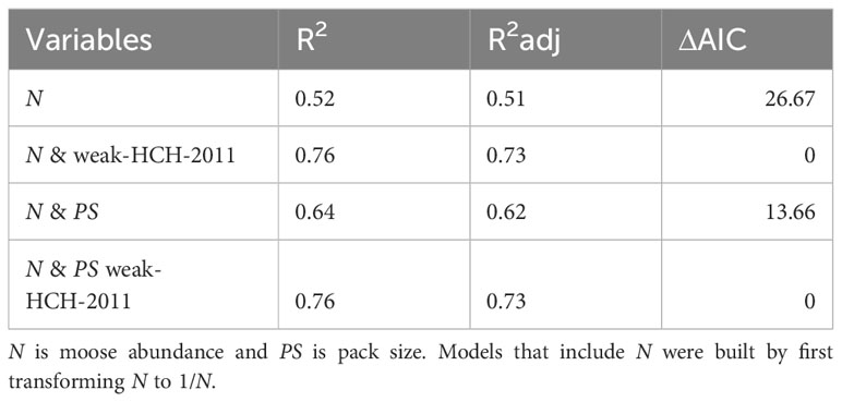
Table 3 Performance of models built to assess the weak historical contingency hypothesis.

Reddened spectra

Lastly, we investigated the relationship between historical contingencies and reddened spectra. Specifically, we assessed whether four essential elements of predator-prey dynamics on Isle Royale (N, P, KR and PR) showed signs of reddened spectra. We followed Ariño and Pimm (1995) and assessed reddened spectra with plots showing how the sample variance of each of the four elements changes with the length of observation. Time series are considered to exhibit reddened spectra if they show a continued increase of interannual variation, with no evidence of reaching an asymptote. We then observed how historically contingent events coincided with temporal patterns in variance.

Several of the time-series showed signs of reddened spectra insomuch as they did not reach an asymptote over the study period (Figure 1, lower panel). Furthermore, each historically contingent event (A-E) was immediately preceded by an abrupt increase in variance in at least one of the four elements. For example, event (A) was preceded by an abrupt increase in the variance of P; event (B) was preceded by an abrupt increase in the variance of PR and N; and event (D) was preceded by an abrupt increase in the variance in KR.

Discussion

In summary, we developed a novel conceptualization of historical contingencies and a simple approach for quantifying the importance of historical contingencies for explaining elements of population ecology. We applied those ideas to a case-study (wolves and moose on Isle Royale) and found that the HCH models were better than, or at least competitive with, all of the alternative theory-based models that we assessed. We also found evidence suggesting that there may be a relationship between historical contingencies and reddened spectra. While broad claims about the HCH cannot be satisfactorily evaluated with a single study system, we provide the means for follow-up analyses because this method can be applied to any population that has been studied in reasonable detail over a long period of time [such as those referenced in (Clutton-Brock and Sheldon, 2010)].

Several essential results situate the importance of historical contingencies for explaining the predator-prey dynamics studied here. First, models associated with the strong HCH explained over half of the interannual variation in predation rate and out-performed theory-based models designed to assess some of the most important mechanisms in predation ecology (Table 1). Second, models associated with the weak HCH, that account for both historical contingencies and key ecological mechanisms, explained substantially more variance than models which only accounted for mechanisms (Table 3). While solid support for the weak HCH is not surprising, the impressive performance of the strong HCH model is remarkable. The impressive performance of the HCH models does not diminish the value of models representing ecological theory. rather, our results highlight the importance of historical contingency, especially in relationship to ecological theory. For emphasis, we are not supposing, nor should it be supposed, that ecological theory and HCH are mutually exclusive explanations.

When comparing the HCH models to alternative models, it is important to consider the purpose of those alternative models and the means by which they were obtained. In particular, a few models in Table 2 had higher R² and lower AIC values than the strong HCH models. However, those models were found by data dredging which is known to produce models that are overfit, resulting in inflated values of R² and deflated values of AIC. More importantly, there is a high degree of statistical dependence between the response and predictor variables contained in the alternative models with the highest R² and lowest AIC.

The strong HCH models also compare interestingly with the cross-validated model, whose explicit purpose is to make a forecast. First, although the HCH models seem as though they demand a great deal of data, it is important to observe that cross-validation is similarly demanding of data. Second, the cross-validated model performed very well on the training data (R² = 0.80), but very poorly on the test data (R² = 0.13). That disparity is likely because the system experienced alternative stable states (see below). In other words, the reason why the forecast was very poor is precisely for the same reason that the HCH model performed so well.

HCH as synthesis

The HCH is also a framework for synthesizing several ecological phenomena of broad significance. For example, we show connections between historical contingencies and reddened spectra (Figure 1). The broader significance of reddened spectra is indicated by their influence on resilience and extinction risk (Schwager et al., 2006; Ponciano et al., 2018) and their association with ecological surprises (Ariño and Pimm, 1995).

The HCH also assimilates legacy effects, tipping points and alternate stable state theory. For example, the historical periods we observed are aptly characterized as alternate states, represented as periods of strong top-down regulation (periods I and III) and periods of weak regulation by predation (periods II and IV; Figures 1, 2). Furthermore, simulations indicate that shifts between stable states are likely to be preceded by periods of increased variance (Carpenter and Brock, 2006). We provide rare empirical evidence supporting the results of those simulations by showing that periods defined, a priori, by historically-contingent events were immediately preceded by an abrupt increase in variance for some, but not all, elements of the system (Figure 1, lower panel). These abrupt increases in variance may be linked to the waning legacies of previous historically-contingent events. More importantly, we observed at least three shifts over the five-decade study period (i.e., after events A, B/C, D). That observation advances understanding of alternate stable state theory by providing a benchmark for understanding how frequently such shifts may occur. At present, few systems have been studied in sufficient detail and over long enough time periods to observe three or more alternate stable states.

Several of the historically-contingent events that we observed were the seemingly unlikely coincidence of multiple events. Specifically, Event A is the coincidence of a novel disease and the highest predator abundance ever observed in this system. Event B is the coincidence of an extreme winter and the highest prey abundance ever observed in this system and then event C (genetic rescue in the wolf population) occurred only a year later. Therefore, much that has occurred in this system is attributable to these seemingly unlikely coincidences which consist of either compounding or countervailing influences (for details, see Supplementary Materials). That observation is consistent with earlier work indicating that coincidences with compounding influences can have important effects (Denny et al., 2009). That observation also offers critical perspective to prior work indicating that synergies tend to result in ecological surprises, but the occurrence of synergies is rarer than is often supposed (Côté et al., 2016). The rarity of synergies arises from its narrow (albeit appropriate) definition, i.e., two or more events combining to result in a super-additive effect (Brook et al., 2008). The coincidences that we observed were impressively impactful without necessarily being concerned with whether they were synergies with super-additive effects. Furthermore, the observation of several seemingly unlikely coincidences over six decades suggests a need to better judge whether the coincidences were genuinely unlikely or only seemingly so. The apparent discrepancy is resolved by noting the disparate nature of the events involved (extreme winter, novel disease, immigration events). Because ecosystems are composed of such a vast array of biotic and abiotic influences, it is not surprising to observe coincidences like those observed here with some regularity. Therefore, one should expect seemingly unlikely coincidences to occur periodically and that they may have an important influence on population dynamics [see also (Paine et al., 1998; Denny et al., 2009)].

HCH, forecasting, & surprises

Our results also suggest that the HCH is a valuable explanation for why “ecological surprises” are so frequent (i.e., because of the disparate nature of coincidences that can have important impacts) and their inordinate influence. In this way, the HCH is similar to the Black Swan Theory of Events which was developed to explain the behavior of financial markets (Taleb, 2010). More precisely, the Black Swan Theory aims to explain the inordinate influence of events that cannot be reliably forecast from historical patterns, as well as the psychological biases that limit humans’ ability to appreciate the unpredictability and import of such events. According to this theory, black swan events are rare, unpredictable events with dramatic, and often catastrophic impacts. Additionally, black swan events are explained only with the benefit of hindsight, but in such a way that misleads financial managers and stakeholders to believe and act as though such events could have been forecast. A key difference between the HCH and Black Swan Theory is that the latter is centered on explaining the limits of human perception. However, the HCH and Black Swan Theory both call for a richer acknowledgement and appreciation of unpredictable events so that people do not underestimate the vulnerability of systems.

A recent study concluded that black swan events are rare in ecology (Anderson et al., 2017). However, that study conceptualized black swan events as heavy-tailed process noise in time series of population abundance without requiring that the cause of any heavy-tailed process noise be known or identifiable. Heavy-tailed process noise was detected in only 4% of the 609 time series analyzed and it was less likely to be detected it in short times series. The median length of the time series was relatively short (i.e., ~26 years). The shortness of time series analyzed and the narrow definition of black swan events used in that study may have resulted in the frequency of black swan events in ecology being underestimated. Moreover, detecting black swan events may require more information than is contained in simple time series data. Although the statistical patterns observed by (Anderson et al., 2017) are important and valuable, they could lead to a misunderstanding of how common important and unexpected events are in ecology.

Future assessments

Broad claims about the HCH cannot be satisfactorily evaluated with a single system. However, our method could be applied to any population that has been studied over a long period of time and in reasonable detail, such that understanding of the system transcends simple time series data. While the prevalence of such data shouldn’t be prejudged, it may prove to be rare. In that case, testing the HCH would be greatly challenged by the paucity of data. The paucity of existing data to test a new hypothesis is independent from the hypotheses’ value. Rather the basis for judging the value of any hypothesis is: is the hypothesis plausibly true, and would discovering the extent of its truth yield worthwhile knowledge? If the answer to those questions is yes, and if the data needed to test the hypothesis do not exist, then the traditional development in science is to begin collecting such data. That such data collection might be difficult or slow seems less pertinent. In this vein, an ancillary value of this hypothesis may be, as detailed in (Vucetich et al., 2020): (i) to provide more reason for ecologists to begin prioritizing the development of long-term ecological research, and (ii) to stimulate more discussion about how to most effectively conduct long-term ecological research – because all approaches to such research may not be equally effective.

At this early stage of considering the HCH, it is natural to ask, what types of systems are mostly likely explained by the HCH? It seems plausible that the HCH is likely to have explanatory power in systems prone to exhibiting ecological surprises or alternative stable states – perhaps because they are exposed to the kinds of (exogenous) forces that are most likely to represent tipping points. Systems that exhibit reddened spectra would also seem to be prime candidates for being explained by the HCH. One would not expect a population’s dynamics to be explained by the HCH if it had only been monitored for a relatively short time (e.g. a decade or 3 generations) because not enough time is likely to have passed for multiple historically contingent events to occur and have long-lasting legacy effects.

We suppose that future assessments of the HCH would have two elements, a model representing the HCH and at least one, directly comparable, alternative model representing the most appropriate ecological theory given the system being assessed. By directly comparable, we mean that the response variable for both models would be the same data (in our case, predation rate for a specified period of time). The model representing HCH should be built – we suppose – as we did here, by identifying events that had important and long-lasting effects which divide time series into segments and do so without cherry-picking events simply because they minimize the models AIC. This description should be accompanied by two caveats. First, the assessment of a hypothesis – including the HCH – is always provisional. The conclusion that HCH is (or is not) important can be revised by future testing, which may involve more data or the discovery of different models to better represent HCH. Second, we expect others may develop alternative means of testing the HCH. These alternatives may even lead to refinements in the hypothesis itself. That expectation is consistent with the development of other ideas in population biology, such as standards of evidence for genetic rescue (Hedrick et al., 2011) and trophic cascades (Peterson et al., 2014).

Lastly, our case shows how legacy effects or the occurrence of some events may not easily be defined by a single year, as was the case for the end of period III and start of period IV (Figure 1; Table 1). Nevertheless, the statistical framework presented here favors identifying a precise year. In our case study, the R² value of the HCH models varies somewhat (0.53 to 0.59), depending on when we suppose that period III ended and period IV began (2009, 2010, or 2011). However, the salient point is that the various values of R² for those three HCH models are all consistent with the ultimate conclusion of the paper, i.e., the models representing the HCH explain about half of the variation in PR and perform better than, or are at least competitive with, all of the other models that we assessed. Nevertheless, it is imaginable that other cases may require a more complex statistical model to represent the HCH.

Conclusion

Overall, we found strong evidence supporting the HCH for this case study and our results suggest that a large class of ecological phenomena are synthesized by the HCH. In community ecology, Losos (1994) concluded that: “only rarely will ecological forces be so strong as to completely erase the vestiges of history”. Our work suggests that the influence of historical contingency could be equally as strong for population ecology. If the HCH were found to be broadly applicable, it would explain one of the most basic features of ecological science. That is, why ecologists can so effectively explain population dynamics with hindcasts, but are conspicuously poor at forecasting. The plausibility of the HCH and the elements it synthesizes – reddened spectra, tipping points, etc. – provide even more reason to be humble about our inherent limitations to forecasting and to stop overestimating our ability to control ecosystems.

Data availability statement

Publicly available datasets were analyzed in this study. This data can be found here: https://isleroyalewolf.org/data/data/home.html, https://wrcc.dri.edu/spi/divplot1map.html, and https://climatedataguide.ucar.edu/climate-data/hurrell-north-atlantic-oscillation-nao-index-station-based.

Ethics statement

The animal study was approved by the IACUC Committee at Michigan Technological University. The study was conducted in accordance with the local legislation and institutional requirements.

Author contributions

SH: Conceptualization, Data curation, Formal Analysis, Investigation, Methodology, Project administration, Visualization, Writing – review & editing. RP: Data curation, Funding acquisition, Investigation, Methodology, Project administration, Resources, Writing – review & editing. JV: Conceptualization, Data curation, Funding acquisition, Investigation, Methodology, Project administration, Resources, Validation, Writing – original draft.

Funding

The author(s) declare financial support was received for the research, authorship, and/or publication of this article. This conceptualization of the HCH was developed as part of a grant funded by the U.S. National Science Foundation (DEB-1453041 to JV). This work was also supported by Isle Royale National Park (CESU Task Agreement No P22AC00193 to SH), a McIntyre-Stennis Grant (USDA-Nifa#1004363 to JV), Robert Bateman Endowment at the Michigan Tech Fund, James L. Bigley Revocable Trust, and Detroit Zoological Society and private donations. Support for RP came from the Robbins Chair in Environmental Sustainability.

Acknowledgments

We are grateful to the many individuals who contributed to the collection of field data. The views expressed here do not necessarily reflect those of the U.S. National Park Service.

Conflict of interest

The authors declare that the research was conducted in the absence of any commercial or financial relationships that could be construed as a potential conflict of interest.

Publisher’s note

All claims expressed in this article are solely those of the authors and do not necessarily represent those of their affiliated organizations, or those of the publisher, the editors and the reviewers. Any product that may be evaluated in this article, or claim that may be made by its manufacturer, is not guaranteed or endorsed by the publisher.

Supplementary material

The Supplementary Material for this article can be found online at: https://www.frontiersin.org/articles/10.3389/fevo.2024.1325248/full#supplementary-material

References

Abrams P. (1993). Why predation rate should not be proportional to predator density. Ecology 74, (3) 726–733.
Abrams P., Ginzburg L. R. (2000). The nature of predation: Prey dependent, ratio dependent or neither? Trends Ecol. Evolution. 15, (8) 337–341.
Akçakaya H. R., Halley J. M., Inchausti P. (2003). Population-level mechanisms for reddened spectra in ecological time series. J. Anim. Ecol. 72, 698–702. doi: 10.1046/j.1365-2656.2003.00738.x
Anderson S. C., Branch T. A., Cooper A. B., Dulvy N. K. (2017). Black-swan events in animal populations. Proc. Natl. Acad. Sci. U. S. A. 114, 3252–3257. doi: 10.1073/pnas.1611525114
Arditi R., Ginzburg L. R. (1989). Coupling in predator-prey dynamics: Ratio-Dependence. J. Theor. Biol. 139, (3) 311–326.
Ariño A., Pimm S. L. (1995). On the nature of population extremes. Evol. Ecol. 9, 429–443. doi: 10.1007/BF01237765
Beckage B., Gross L. J., Kauffman S. (2011). The limits to prediction in ecological systems. Ecosphere 2, 1–12. doi: 10.1890/ES11-00211.1
Beisner B. E., Haydon D. T., Cuddington K. (2003). Alternative stable states in ecology. Front. Ecol. Environ. 1, 376–382. doi: 10.1890/1540-9295(2003)001[0376:ASSIE]2.0.CO;2
Bender E. A., Case T. J., Gilpin M. E. (1984). Perturbation experiments in community ecology: theory and practice. Ecology 65, 1–13. doi: 10.2307/1939452
Berryman A. A. (2003). On principles, laws and theory in population ecology. Oikos 103, 695–701. doi: 10.1034/j.1600-0706.2003.12810.x
Brook B. W., Sodhi N. S., Bradshaw C. J. A. (2008). Synergies among extinction drivers under global change. Trends Ecol. Evol. 23, 453–460. doi: 10.1016/j.tree.2008.03.011
Carpenter S. R., Brock W. A. (2006). Rising variance: a leading indicator of ecological transition. Ecol. Lett. 9, 311–318. doi: 10.1111/j.1461-0248.2005.00877.x
Clutton-Brock T., Sheldon B. C. (2010). Individuals and populations: the role of long-term, individual-based studies of animals in ecology and evolutionary biology. Trends Ecol. Evol. 25, 562–573. doi: 10.1016/j.tree.2010.08.002
Colyvan M., Ginzburg L. R. (2003). Laws of nature and laws of ecology. Oikos 101, 649–653. doi: 10.1034/j.1600-0706.2003.12349.x
Côté I. M., Darling E. S., Brown C. J. (2016). Interactions among ecosystem stressors and their importance in conservation. Proc. R. Soc B Biol. Sci. 283, 20152592. doi: 10.1098/rspb.2015.2592
Craig E. (1998). “Realism and antirealism,” in The Routledge Encyclopedia of Philosophy. Ed. Craig E. (Routledge, London & New York: Taylor & Francis).
Cuddington K. (2011). Legacy effects: the persistent impact of ecological interactions. Biol. Theory 6 (3), 203–210.
Denny M. W., Hunt L. J. H., Miller L. P., Harley C. D. G. (2009). On the prediction of extreme ecological events. Ecol. Monogr. 79, 397–421. doi: 10.1890/08-0579.1
Doak D. F., Estes J. A., Halpern B. S., Jacob U., Lindberg D. R., Lovvorn J., et al. (2008). Understanding and predicting ecological dynamics: Are major surprises inevitable? Ecology 89, 952–961. doi: 10.1890/07-0965.1
Droghini A., Boutin S. (2018). The calm during the storm: Snowfall events decrease the movement rates of grey wolves (Canis lupus). PloS One 13, e0205742. doi: 10.1371/journal.pone.0205742
Emmerson M. C., Raffaelli D. (2004). Predator-prey body size, interaction strength and the stability of a real food web. J. Anim. Ecol. 73, 399–409. doi: 10.1111/j.0021-8790.2004.00818.x
Fukami T. (2015). Historical contingency in community assembly: integrating niches, species pools, and priority effects. Annu. Rev. Ecol. Evol. Syst. 46, 1–23. doi: 10.1146/annurev-ecolsys-110411-160340
Harrison P. (2016). What was historical about natural history? Contingency and explanation in the science of living things. Stud. Hist. Philos. Sci. Part C Stud. Hist. Philos. Biol. Biomed. Sci. 58, 8–16. doi: 10.1016/j.shpsc.2015.12.012
Hayes R. D., Baer A. M., Harestad A. S. (2000). Kill rate by wolves on moose in the Yukon. Can. J. Zool. 78, 49–59. doi: 10.1139/z99-187
Hedrick P. W., Adams J. R., Vucetich J. A. (2011). Reevaluating and broadening the definition of genetic rescue. Conserv. Biol. 25, 1069–1070. doi: 10.1111/j.1523-1739.2011.01751.x
Hedrick P. W., Kardos M., Peterson R. O., Vucetich J. A. (2017). Genomic variation of inbreeding and ancestry in the remaining two Isle Royale wolves. J. Hered. 108, 120–126. doi: 10.1093/jhered/esw083
Hedrick P. W., Peterson R. O., Vucetich L. M., Adams J. R., Vucetich J. A. (2014). Genetic rescue in Isle Royale wolves: genetic analysis and the collapse of the population. Conserv. Genet. 15, 1111–1121. doi: 10.1007/s10592-014-0604-1
Holling C. (1959). The components of predation as revealed by a study of small-mammal predation of the European Pine Sawfly. Can. Entomologist. 91 (5), 293–320.
Holt R. D. (2008). Theoretical perspectives on resource pulses. Ecology 89, 671–681. doi: 10.1890/07-0348.1
Hoy S. R., Forbey J. S., Melody D. P., Vucetich L. M., Peterson R. O., Koitzsch K. B., et al. (2022). The nutritional condition of moose co-varies with climate, but not with density, predation risk or diet composition. Oikos 1, e08498. doi: 10.1111/OIK.08498
Hoy S. R., Hedrick P. W., Peterson R. O., Vucetich L. M., Brzeski K. E., Vucetich J. A. (2023). The far-reaching effects of genetic process in a keystone predator species, grey wolves. Sci. Adv. 9, eadc8724. doi: 10.1126/sciadv.adc8724
Hoy S. R., Peterson R. O., Vucetich J. A. (2019). Ecological studies of wolves on Isle Royale 2018-2019 (Houghton: Michigan Technological University). doi: 10.37099/mtu.dc.wolf-annualreports/2018-2019
Hoy S. R., Vucetich L. M., Peterson R. O., Vucetich J. A. (2021). Winter tick burdens for moose are positively associated with warmer summers and higher predation rates. Front. Ecol. Evol. 0. doi: 10.3389/fevo.2021.758374
Hurrell J. (1995) Hurrell North Atlantic Oscillation (NAO) Index 390 (station-based). Available online at: https://climatedataguide.ucar.edu/climate-data/hurrellnorth-atlantic-oscillation-nao-index-station-based (Accessed August 31, 2011).
Inamine H., Miller A., Roxburgh S., Buckling A., Shea K. (2022). Pulse and press disturbances have different effects on transient community dynamics. Am. Nat. 200, 571–583. doi: 10.1086/720618
Inchausti P., Halley J. (2001). Investigating long-term ecological variability using the Global Population Dynamics Database. Science 293, 655–657. doi: 10.1126/science.293.5530.655
Inchausti P., Halley J. M. (2002). The long-term temporal variability and spectral colour of animal populations. Evol. Ecol. Res. 4, 1033–1048.
Křivan V. (2008). Prey-predator models. Pages 2929-2940 in S. E. Jørgensen and B. D. Fath, eds. Population Dynamics. Vol. 4 of Encyclopedia of Ecology, 5 vols. Elsevier, Oxford.
Lindstrom J., Kokko H., Ranta E., Linden H. (1999). Density dependence and the response surface methodology. Oikos 85, 40. doi: 10.2307/3546790
Losos J. B. (1994). “Historical contingency and lizard community ecology,” in Lizard Ecology: Historical and Experimental Perspectives. Eds. Vitt L. J., Pianka E. (Princeton University Press, Princeton), 319–333.
Losos J. B. (2010). Adaptive radiation, ecological opportunity, and evolutionary determinism : American society of naturalists E. O. Wilson award address. Am. Nat. 175, 623–639. doi: 10.1086/652433
MacNulty D. R., Smith D. W., Mech L. D., Vucetich J. A., Packer C. (2012). Nonlinear effects of group size on the success of wolves hunting elk. Behav. Ecol. 23, 75–82. doi: 10.1093/beheco/arr159
McLaren B., Peterson R. (1994). Wolves, moose, and tree rings on Isle Royale. Science 266, 1555–1558. doi: 10.1126/science.266.5190.1555
Messier F. (1994). Ungulate population models with predation: a case study with the North American moose. Ecology 75 (2), 478–488.
Moorhead D. L., Doran P. T., Fountain A. G., Lyons W. B., Mcknight D. M., Priscu J. C., et al. (1999). Ecological legacies: impacts on ecosystems of the McMurdo dry valleys. BioScience 49, (12) 1009–1019.
Paine R. T., Tegner M. J., Johnson E. A. (1998). Compounded perturbations yield ecological surprises. Ecosystems 1, 535–545. doi: 10.1007/s100219900049
Parker K. L., Barboza P. S., Gillingham M. P. (2009). Nutrition integrates environmental responses of ungulates. Funct. Ecol. 23, 57–69. doi: 10.1111/j.1365-2435.2009.01528.x
Peterson R. O. (1996). Ecological Studies of Wolves on Isle Royale (Houghton, MI: Michigan Technological University). doi: 10.37099/mtu.dc.wolf-annualreports/1995-1996
Peterson R. O., Page R. E. (1988). The rise and fall of Isle Royale wolves 1975-1986. J. Mammal. 69, 89–99. doi: 10.2307/1381751
Peterson R. O., Page R. E. (1993). Detection of moose in midwinter from fixed-wing aircraft over dense forest cover. Wildl. Soc Bull. 21, 80–86.
Peterson R. O., Thomas N. J., Thurber J. M., Vucetich J. A., Waite T. A. (1998). Population limitation and the wolves of Isle Royale. J. Mammal. 79, 828–841. doi: 10.2307/1383091
Peterson R. O., Vucetich J. A. (2014). Ecological studies of wolves on Isle Royale: Annual report 2013–14 (Houghton: Michigan Technological University).
Peterson R. O., Vucetich J. A., Bump J. M., Smith D. W. (2014). Trophic cascades in a multicausal world: Isle Royale and Yellowstone. Annu. Rev. Ecol. Evol. Syst. 45, 325–345. doi: 10.1146/annurev-ecolsys-120213-091634
Ponciano J. M., Taper M. L., Dennis B. (2018). Ecological change points: The strength of density dependence and the loss of history. Theor. Popul. Biol. 121, 45–59. doi: 10.1016/j.tpb.2018.04.002
Poole R. W. (1978). The statistical prediction of population fluctuations. Annu. Rev. Ecol. Syst. 9, 427–448. doi: 10.1146/annurev.es.09.110178.002235
Ritson S., Staley K. (2021). How uncertainty can save measurement from circularity and holism. Stud. Hist. Philos. Sci. 85, 155–165. doi: 10.1016/j.shpsa.2020.10.004
Scheffer M., Bascompte J., Brock W. A., Brovkin V., Carpenter S. R., Dakos V., et al. (2009). Early-warning signals for critical transitions. Nature 461, 53–59. doi: 10.1038/nature08227
Schmitz O. J. (2010) Resolving Ecosystem Complexity (New Jersey: Princeton University Press). Available online at: https://press.princeton.edu/books/paperback/9780691128498/resolving-ecosystem-complexity-mpb-47 (Accessed July 17, 2020).
Shrader-Frechette K. S., McCoy E. D. (1993). Method in ecology (Cambridge: Cambridge University Press).
Schoener T. W. (1986). Mechanistic approaches to community ecology: A new reductionism? Am. Zool. 26, 81–106. doi: 10.1093/icb/26.1.81
Schwager M., Johst K., Jeltsch F. (2006). Does red noise increase or decrease extinction risk? Single extreme events versus a series of unfavorable conditions. Am. Nat. 167, 879–888. doi: 10.1086/503609
Selkoe K. A., Blenckner T., Caldwell M. R., Crowder L. B., Erickson A. L., Essington T. E., et al. (2015). Principles for managing marine ecosystems prone to tipping points. Ecosyst. Heal. Sustain. 1, 17–18. doi: 10.1890/EHS14-0024.1
Simberloff D. (2004). Community ecology: is it time to move on? American Naturalis 163 (6), 787–799. doi: 10.1086/420777
Turchin P. (2001). Does population ecology have general laws? Oikos 94, 17–26. doi: 10.1034/j.1600-0706.2001.11310.x
Vucetich J. A., Hebblewhite M., Smith D. W., Peterson R. O. (2001). Predicting prey population dynamics from kill rate, predation rate and predator-prey ratios in three wolf-ungulate systems. J. Anim. Ecol. 80 (6), 1236–1245.
Vucetich J. A. (2021). Restoring the balance: what wolves tell us about our relationship with nature (Baltimore, Maryland: Johns Hopkins University Press).
Vucetich J. A., Peterson R. O. (2004). The influence of prey consumption and demographic stochasticity on population growth rate of Isle Royale wolves Canis lupus. Oikos 107, 309–320.
Vucetich J. A., Hebblewhite M., Smith D. W., Peterson R. O. (2011). Predicting prey population dynamics from kill rate, predation rate and predator-prey ratios in three wolf-ungulate systems. J. Anim. Ecol. 80, 1236–1245. doi: 10.1111/jane.2011.80.issue-6
Vucetich J. A., Nelson M. P., Bruskotter J. T. (2020). What drives declining support for long-term ecological research? Bioscience 70, 168–173. doi: 10.1093/biosci/biz151
Vucetich J. A., Peterson R. O. (2008). Ecological studies of wolves on Isle Royale (Houghton: Michigan Technological University). doi: 10.37099/mtu.dc.wolf-annualreports/2007-2008
Weladji R. B., Klein D. R., Holand Ø., Mysterud A. (2002). Comparative response of Rangifer tarandus and other northern ungulates to climatic variability. Rangifer 22, 33–50. doi: 10.7557/2.22.1.686
Western Regional Climate Center (2016) Cooperative climatological data summaries. Available online at: https://wrcc.dri.edu/spi/divplot1map.html.
Wilmers C. C., Post E., Peterson R. O., Vucetich J. A. (2006). Predator disease out-break modulates top-down, bottom-up and climatic effects on herbivore population dynamics. Ecol. Lett. 9, 383–389. doi: 10.1111/j.1461-0248.2006.00890.x
Keywords: Black Swan events, resiliency, laws of nature, predation rate, legacy effects, alternative stable states, wolves, moose
Citation: Hoy SR, Peterson RO and Vucetich JA (2024) A historical contingency hypothesis for population ecology. Front. Ecol. Evol. 12:1325248. doi: 10.3389/fevo.2024.1325248
Received: 20 October 2023; Accepted: 29 February 2024;
Published: 14 March 2024.
Edited by:
Dennis Murray, Trent University, CanadaCopyright © 2024 Hoy, Peterson and Vucetich. This is an open-access article distributed under the terms of the Creative Commons Attribution License (CC BY). The use, distribution or reproduction in other forums is permitted, provided the original author(s) and the copyright owner(s) are credited and that the original publication in this journal is cited, in accordance with accepted academic practice. No use, distribution or reproduction is permitted which does not comply with these terms.
*Correspondence: Sarah R. Hoy, srhoy@mtu.edu