Trade Agreements and Financial Market Integration in Latin America and the US

Abstract

The primary objective of this study is to examine the extent of financial integration between Latin American and US financial markets, particularly in light of recent efforts to foster integration through trade agreements. Spanning from 1 January 1990 to 31 December 2019, the sample focuses on major market indices and key sectors. Financial integration is quantified using a DCC multivariate GARCH model, incorporating a smooth transition model, structural breaks, and regression-based approaches. Results indicate increased comovement with the US for main market indices in Argentina, Chile, Colombia, Mexico, and Peru, while Brazil shows a decrease. Similar trends are observed in sectoral analyses. This study also reveals heightened correlation post-trade agreements. Structural break analysis highlights significant shifts in dynamic correlations for countries with US free trade agreements. These findings support the argument of increased financial integration, bearing significance for portfolio diversification and international policy formulation.

1. Introduction

Financial market integration has been a topic of great interest among academicians and practitioners as it directly impacts investments across the world. Financial integration among countries is significant in many aspects of financial economics. For policymakers, understanding the impact that other countries have on their financial market, hence the country’s economy, is of utmost importance. For investors, well-diversified portfolios are created under the idea that correlations are understood, but if these correlations are changing over time, then portfolios should be adjusted based on the time-varying fluctuations of these correlations.

It is important to point out that financial market integration can be measured through several approaches. This investigation focused mainly on one specific measure, comovement, of financial markets. The previous literature has examined the level of comovement within developed countries (Berben and Jansen 2005; Longin and Solnik 1995; Eun and Shim 1989; Shin and Sohn 2006; Rua and Nunes 2009). The results support the argument that market integration is time-varying and that the degree of comovement among financial markets in developed countries is increasing. Most of these studies have focused on financial integration between major developed countries. However, financial market integration between emerging economies has not been examined as thoroughly as developed markets in recent time, even though investors are flocking towards international investments seeking a higher degree of diversification. Forbes and Rigobon (2002) study comovement among international stock markets and find that correlation coefficients are conditional on the examined markets’ volatility. In addition, Bekaert and Harvey (1995) show that some Latin American equity markets tend to have a low correlation with the US, while Johnson and Soenen (2003) show that Latin American markets’ comovement with the US is changing in different directions. Also, Fujii (2005) investigate the links between selected Asian and Latin American countries and find significant market connections between the examined Asian and Latin American markets.

There is a substantial amount of recent literature studying the relationship between trade integration and financial integration. Vo (2022) investigates this relationship in Asia using a dataset covering the period from 2001 to 2015. They find a positive and significant bidirectional relationship between international trade integration and international financial integration. Abbasov (2019) found that trade integration has a positive effect on financial integration in both the short and long term for OECD and G20 countries during 2000–2016. Erkut and Sharma (2023) study whether the degree of trade integration in Asia also spills over to financial integration by focusing on Asian trade production networks. Didier et al. (2017) examine the complementarity between trade and financial flows in East Asia and the Pacific. Lim and Breuer (2019) find evidence that after free trade agreements, trade costs have been reduced for nine countries, providing evidence that greater market integration has been achieved in South Korea. Wang et al. (2023) analyze how the deepening of free trade agreements promotes the growth of China’s international trade.

Latin American countries have been working to integrate their main financial markets. These efforts have increased access to capital for both domestic and international firms. For example, the creation of the Mercado Integrado Latinoamericano (MILA), which is an integrated exchange that consists of four of the most relevant markets in the region (Chile, Colombia, Mexico, and Peru). With this new integration, stocks from all these countries can be traded by investors in any of the four markets in their original currency. Further, regional cooperation organizations like Latin American Integration Association (ALADI) or Mercosur (South American Common Market) have helped unite these countries in a wide range of factors. These efforts have also focused on aiding economies and financial markets to interact more closely within this region.

In addition, regional trading deals such as the North American Free Trade Agreement (NAFTA), which involves a direct free trade agreement between Canada, the US, and Mexico, was established in 1994. This trade agreement included tariff reductions for a significant number of goods between these countries that were gradually reduced until 2008. In 2019, a new NAFTA deal is being prepared.1 This was the initial free trade agreement between the US and any Latin American country. The US government has gradually increased trade and cooperation efforts with several countries in this region by creating trade agreements with a significant number of countries in Central and South America.

The US has put in place several bilateral trade agreements with countries in this region. For example, the US government has utilized three main types of trade agreements with countries in the Latin American region, which are: the Trade and Investment Framework Agreement (TIFA), Agreement on Trade and Economic Cooperation (ATEC), and bilateral Free Trade Agreements (FTA). A Trade and Investment Framework Agreement (TIFA) is considered a trade deal that creates a strategic framework to expand trade and resolve any disputes between countries. The Agreement on Trade and Economic Cooperation (ATEC) created between Brazil and the US is a specific agreement between these countries. The ATEC is a unique pact in the sense that it promotes bilateral trade and economic cooperation, but it is not a full free trade agreement. In essence, the agreement is very similar to a Trade and Investment Framework Agreement (TIFA), and it is perceived as a first step towards the creation of a future free trade agreement between both countries. These agreements tend to pave the way for bilateral free trade agreements with the US. A free trade agreement is a trade deal that diminishes barriers of imports and exports. Under a free trade agreement, goods and services can be exchanged across countries’ borders with minimal or no government tariffs, quotas, subsidies, or prohibitions. This type of trade pact is the strongest among the three different types the US has used within this region. Nonetheless, all the above-mentioned trade agreements intend to reduce trade and investment barriers, open markets, and eliminate obstacles between these two countries over time.

Specifically in this region, the US has created three different free trade agreements. NAFTA includes three countries (the US, Mexico, and Canada), while the remaining deals are bilateral free trade agreements. The US has a bilateral free trade agreement with Chile, Colombia, and Peru. Moreover, The United States–Chile Free Trade Agreement (FTA) entered into force on 1 January 2004, but the deal was signed on 6 March 2003. The United States–Colombia Trade Promotion Agreement (FTA) was signed on 22 November 2006, but took about 6 years to put into force on 15 May 2012. Of the bilateral free trade agreements, the Colombian pact took the longest to get implemented after the official signature between the countries. The United States–Peru Free Trade Agreement (FTA) entered into force on 1 February 2009, while it was initially agreed upon on 12 April 2006. On the other hand, the US has also instituted a TIFA and an ATEC with Argentina and Brazil, respectively. On 18 March 2011, the US and Brazil signed an Agreement on Trade and Economic Cooperation (ATEC) to strengthen trade and investment between the two nations. Finally, Argentina and the US signed a bilateral Trade and Investment Framework Agreement (TIFA) on 23 March 2016 to advance trade and market accessibility between both countries.2 As a result, these trade agreements have strengthened the ties between the US and these six countries on a wide range of levels, sectors, and industries.

All these integration efforts have been of great importance considering the close geographical proximity between these countries. For instance, Bae et al. (2019) state that most Latin American countries import heavily from the US. According to Bae et al. (2019), the US is the largest importer for all the Latin American countries examined in this paper, which shows these countries are deeply connected in a wide range of levels. According to Forbes and Chinn (2004), trade flows are one of the most relevant determinants of cross-country relations. Basnet and Sharma (2013) examine the integration in terms of macro variables (i.e., GDP, Investment, Trade, and Consumption) between the major Latin American countries, and this study concludes that these countries are getting a higher degree of synchronization both in the short and long term. Consequently, the expectation is that the trade agreements are able to help these countries accelerate integration among the studied stock markets.

Whether the degree of comovement has increased or decreased, it is of great importance to closely examine these correlations to determine how to properly construct portfolios. This has been overlooked due to their market size and slow development. Consequently, this study brings a contribution to the existing literature by examining the degree of financial integration, through market comovement, within the stock markets in Latin America as well as their degree of comovement with the American market. In addition, this investigation helps determine how these trade agreements affect financial market integration and if they have been a direct catalyst for a higher or lower degree of integration.

Finally, the main objectives of this paper are twofold. First, to research the level of financial market integration between the US and the main Latin American markets over time. Second, to explore if the different types of trade agreements between the US and these countries have impacted the comovement of these financial markets. This study concludes that the degree of comovement between the US and the main Latin American countries (Argentina, Brazil, Chile, Colombia, Mexico, and Peru) vary widely. Different sectors and industries are affected differently through the sample, and the trade agreements seem to impact sectors that deal with physical products (basic materials, consumer goods, industrial, financial, and energy) more than the others. In terms of the main market indices, the results show that the integration with the American market index (S&P 500) has increased over time for all the countries except for Brazil, which had a small reduction in correlation during the end of the sample period.

The rest of the study is organized as follows. Section 2 and Section 3 present the methodology and data, respectively. Section 4 reports empirical results. Section 5 offers concluding remarks of this study.

2. Methodology

To thoroughly research the correlations between the returns of the different stock markets, this paper investigates the dynamic conditional correlations between the American market index and sector indices with their Latin American counterparts. This approach will help us determine the level of comovement between the market index as well as different sector indices. In addition, a smooth transitional model is introduced to establish the changes in correlation over time, while structural breaks on this correlation are implemented to determine if the signing and/or implementation of the trade agreements had a direct impact on these correlations. Finally, a regression-based approach is considered to study the degree of comovement before and after the signing and/or implementation of the trade agreements.

As previously mentioned, this paper focuses on one of the most used measures of financial integration: comovement between market indices. For asset return volatility, it is shown that large changes in returns in one period tend to be followed by large changes in the following periods. This is called volatility clustering, which usually becomes more evident as the frequency of the data rises. The GARCH class models have proven to be successful in capturing volatility clustering. As shown in previous studies, GARCH models appear to properly account for the stochastic properties of stock returns and correlation, in other words, time-variation and persistence of the variables.

Taking these properties into account, this paper will follow the dynamic conditional correlation (DCC) approach proposed by Engle (2002). The dynamic conditional correlation model can determine how correlations among the examined countries have changed through the studied sample. Therefore, this model can measure comovement between the US and the Latin American financial markets. The DCC-GARCH model follows:

$$r_t={\mu }_t+{\epsilon }_t,{\epsilon }_t|I_{t-1}\to \mathrm{N}(0,H_t)$$

(1)

where $r_t$ is a $k\times l$ vector that consists of the index return series for each market, and $H_t$ is the conditional variance–covariance matrix of the return vector $r_t$, while ${\epsilon }_t|I_{t-1}$ accounts for the information set that considers all the information up to time t. Further, the conditional variance–covariance matrix can be expressed as follows:

$$H_t=D_t{R}_t{D}_t$$

(2)

and

$$D_t=diag(\sqrt{h_{1t}},\sqrt{h_{2t}})$$

(3)

where $D_t$ is the $2\times 2$ diagonal matrix of time-varying standard deviations from the univariate GARCH models with $\sqrt{h_{it}}$ on the diagonal, and $R_t$ is considered the time variant conditional correlation matrix. Thus, we first estimate the univariate volatility model for each market, and the best one is selected using the Akaike Information Criterion (AIC). The considered models include the GARCH model proposed by Bollerslev (1986), EGARCH model proposed by Nelson (1991), TGARCH proposed by Zakoian (1994) and GJR-GARCH of Glosten et al. (1993). Consequently, the residuals of each are specific market are utilized to estimate the dynamic conditional correlation matrix $R_t$.

The dynamic conditional correlation matrix $R_t$ is expected to change based on a GARCH process and follows:

$$R_t=Q_t^{*-1}{Q}_t{Q}_t^{*-1}$$

(4)

In this case, Q is the unconditional correlation matrix of the $\epsilon$’s and follows:

$$Q_t=\left(1-a-b\right)\overline{Q}+a{\epsilon }_{t-1}^{-1}{\epsilon }_{t-1}^{\prime }+b{Q}_{t-1}$$

(5)

The parameters $a$ and $b$ represent the effect of preceding shocks and former dynamic correlations. These estimates are obtained from the univariate GARCH estimations, and they satisfy $a+b>1$.

The bivariate conditional correlation coefficient ${\rho }_{ij}$ between two markets therefore follows the equation:

$${\rho }_{ij}=\frac{\left(1-a-b\right)\overline{Q}+a{\epsilon }_{t-1}^{-1}{\epsilon }_{t-1}^{\prime }+b{Q}_{t-1}}{\sqrt{\left(1-a-b\right)\overline{Q_{ii}}+a{\epsilon }_{i,t-1}^2+b{Q}_{ii,t-1}}\sqrt{\left(1-a-b\right)\overline{Q_{jj}}+a{\epsilon }_{j,t-1}^2+b{Q}_{jj,t-1}}}$$

(6)

In addition, it is important to examine the effects of free trade agreements within the conditional correlations of the US and these Latin American countries. Therefore, the second approach is to use structural breaks within the dynamic conditional correlations between these countries’ indices. For this approach, two different structures were used. The first one tested for structural breaks for known dates, which in this case, will be the signing date and implementation or start date. The other structure lets the data determine the structural breaks, and the idea is to establish the breaks and their location in a linear regression framework. Following Bai and Perron (2003), if we assume that the dynamic conditional correlations have $m$ number of breaks ($b_1\dots b_m$), then we determine the date of any structural breaks by focusing on the breakpoints that minimize the following function:

$${\widehat{b}}_1\dots {\widehat{b}}_m=arg{min}_{{\widehat{b}}_1\dots {\widehat{b}}_m}{RSS}_{{\widehat{b}}_1\dots {\widehat{b}}_m}$$

(7)

where RSS is the residual sum of squares that results from the $b$ regressions. These regressions that the following form:

$$y_t=\beta x_t^T+{ϵ}_t;(t=1,2,\dots ,n)$$

(8)

In this case, the $y_t$ is the estimated bivariate dynamic conditional correlation series at time $t$, $x_t$ is a vector of the observations of $y_{t-1}$, $\beta$ is the vector of regression coefficients, and ${ϵ}_t$ is the error term which is assumed to be independent and identically distributed ($0,{\delta }^2$).

The null hypothesis states that there is no structural break, while the alternative hypothesis is that the regression coefficients vary over time. Therefore, if we reject the null, then we conclude that the estimated structural break is statistically significant. The idea is to determine if a structural change occurred around the trade agreements.

Structural breaks assume that changes in comovement are instantaneous and readily visible. This might not always be the case considering that these markets can gradually integrate rather than at a determined point in time, regardless of external shocks that impact integration. As a result, the structural breaks approach has several limitations that can be mitigated using other methods. One of those methods is the smooth transition model. The idea behind the smooth transition model is to measure the changes in comovement in an extended period rather than at a specific moment in time. This long-term approach gives a better understanding of the movement between the examined markets as the models show the change in comovement over time.

In addition, other researchers have examined DCC-GARCH models with a smooth transition model to detect structure changes in the correlations (Chelley-Steeley 2005; Berben and Jansen 2005; Lin and Teräsvirta 1994). However, a disadvantage of the smooth transition model is that it assumes a single transition period between two long-run means. This model specification can limit the number of structural changes in the correlation in our sample considering the sample covers an extensive amount of time. The smooth transition model is applied to bivariate equity market dynamic conditional correlations, which have been obtained using the previously discussed dynamic conditional correlation (DCC-GARCH) model.

The logistic smooth transition regression model for the conditional correlations time series between the US and the Latin American countries, ${\rho }_{ij,t}$ estimated earlier, can be expressed as:

$${\widehat{\rho }}_{i{j}_{2}t}=\alpha +\beta S_t\left(\gamma ,\mathsf{\tau }\right)+{ϵ}_t$$

(9)

where ${ϵ}_t$ is considered a stationary ($I\left(0\right)$) process with zero mean. Consequently, the smooth transition between the two examined indices is commanded by the log function $S_t\left(\gamma ,\mathsf{\tau }\right)$. This log function can then be formalized using the following equation:

$$S_t\left(\gamma ,\mathsf{\tau }\right)=1+\exp {\left(-\gamma \left(t-\mathsf{\tau }N\right)\right)}^{-1};(r>1)$$

(10)

where $N$ is the size of the sample. Further, $\mathsf{\tau }$ establishes the point in which the dynamic conditional correlation changed from pattern one to pattern two. In other words, $\mathsf{\tau }$ determined the midpoint or the point of change between the dynamic conditional correlations. The midpoint essentially partitions the sample into a section before integration and section after the integration. Therefore, there is a before and an after in terms of average correlation. The $a$ represents the mean of the section of the sample before the midpoint or old structure before integration, while $\beta$ determines the change in correlations of the sample after the midpoint or turning point, as shown by the smooth transition model. Consequently, if $\beta >0$, then we can conclude that the newer conditional correlation or the correlation after the midpoint has increased through the sample. On the other hand, if $\beta <0$, it means that the newer conditional correlation or the correlation after the midpoint has decreased compared to the initial section. As a result, the summation between $a$ and $\beta$ signifies the mean of the new regime. This method gives us an idea regarding the integration changes over time as well as after the trade agreement.

Although the smooth transition model is able to give us a better representation of the different regimes of correlation, it is also important to note that this approach specifies one single midpoint that serves as the turning point between the changes in correlation. Considering the large time frame, the turning point could appear at any given point in our sample. To determine if dynamic conditional correlations have changed over time, a regression-based approach is taken into consideration. This approach follows:

$$y_t={\alpha }_1+{\delta }_1{\alpha }_2+{ϵ}_t$$

(11)

where $y_t$ is the dynamic conditional correlations previously computed, $\delta$ is the dummy variable indicating the date after the signing or start date of the trade agreement between the US and the given Latin American country, while ${\alpha }_1$ is the constant and ${\alpha }_2$ is the coefficient that determines the increase or decrease after the trade agreement. A positive ${\alpha }_2$ indicates an increase in correlation after the trade agreement, while a negative ${\alpha }_2$ shows a decrease in correlation after the trade agreement. Finally, ${ϵ}_t$ represents the error term.

3. Data

The data used for this study were collected from DataStream. The most important stock exchange markets in Latin America were selected for this research. The selection was based on market capitalization and data availability and includes the following countries: Argentina, Brazil, Chile, Colombia, Mexico, and Peru. The market indices selected for the mentioned nations are: MERVAL for Argentina, IBOVESPA or B3 for Brazil, IPSA for Chile, COLCAP for Colombia, IPC for Mexico, and SPBLPGPT for Peru. On the other hand, the two main American market indices in the US were obtained (S&P500 and DJIA).3

In addition, for each country, the main industry sectors were considered. Following the industry classification benchmark (ICB) used by the FTSE for sector and industry classification, the main industry sectors studied are basic materials, consumer discretionary, consumer staples, energy, financials, healthcare, industrials, real estate, technology, telecommunications, and utilities.4 However, considering that the healthcare and technology sectors are not present in 4 out of the 7 countries, those were not taken into consideration. Further, the real estate index is not available for Colombia, while the energy index is not available for Mexico. The idea is to incorporate as many sectors as possible to research how each different sector comoves with the same sectors in the US. The more sectors incorporated, the better one can understand the different changes in correlations with the US.

The data were selected for the period between 1 January 1990 and 31 December 2019. Although some countries only have data available slightly after the selected starting date; if that is the case, the earliest available data are used. From these data, the daily and weekly returns for each index and sector over the entire sample were computed. Moreover, the log daily and weekly returns were considered as well as the daily and weekly raw returns. The results are consistent, but the weekly log returns were used in this study.5 To eliminate any possible discrepancies with different currencies and to make the returns more comparable, the returns were calculated in US Dollars. As a result, the weekly log returns in USD were used for the entire analysis.

4. Empirical Analysis

4.1. Preliminary Analysis and Time-Varying Estimation Models

Table 1. Summary Statistics. Table 1 reports summary statistics for Latin American countries and the US. In our Latin American data, we have several Latin American countries including Argentina, Brazil, Chile, Colombia, Mexico, and Peru. We first collect daily financial data and then calculate weekly-based log returns and standard deviations sorted by industries. The sample data period is between 1 January 1990 and 31 December 2019.

	Argentina		Brazil		Chile		Colombia		Mexico		Peru		US
	Mean	SD	Mean	SD	Mean	SD	Mean	SD	Mean	SD	Mean	SD	Mean	SD
Market Index	0.059	0.069	0.152	0.058	0.159	0.030	0.097	0.092	0.172	0.045	0.322	0.041	0.141	0.024
Basic Materials	0.047	0.070	0.068	0.055	0.126	0.038	0.199	0.099	0.222	0.050	0.087	0.038	0.119	0.034
Consumer Discretionary	−0.136	0.079	0.149	0.049	0.135	0.041	−0.258	0.105	0.165	0.041	0.249	0.059	0.166	0.024
Consumer Goods	0.104	0.063	0.188	0.047	0.148	0.036	0.049	0.096	−0.115	0.054	0.111	0.034	0.158	0.021
Energy	0.024	0.073	0.170	0.068	0.115	0.042	−0.003	0.102	N/A	N/A	−0.199	0.069	0.099	0.031
Financials	0.054	0.064	0.129	0.054	0.177	0.034	0.063	0.092	0.187	0.048	0.187	0.024	0.142	0.032
Industrials	0.119	0.070	0.198	0.049	0.107	0.038	−0.087	0.056	0.051	0.049	−0.018	0.097	0.176	0.028
Real Estate	−0.004	0.054	0.007	0.055	0.082	0.041	N/A	N/A	−0.022	0.035	0.072	0.020	0.104	0.032
Telecommunications	−0.036	0.064	−0.006	0.053	0.064	0.043	0.024	0.054	0.209	0.048	−0.022	0.066	0.046	0.028
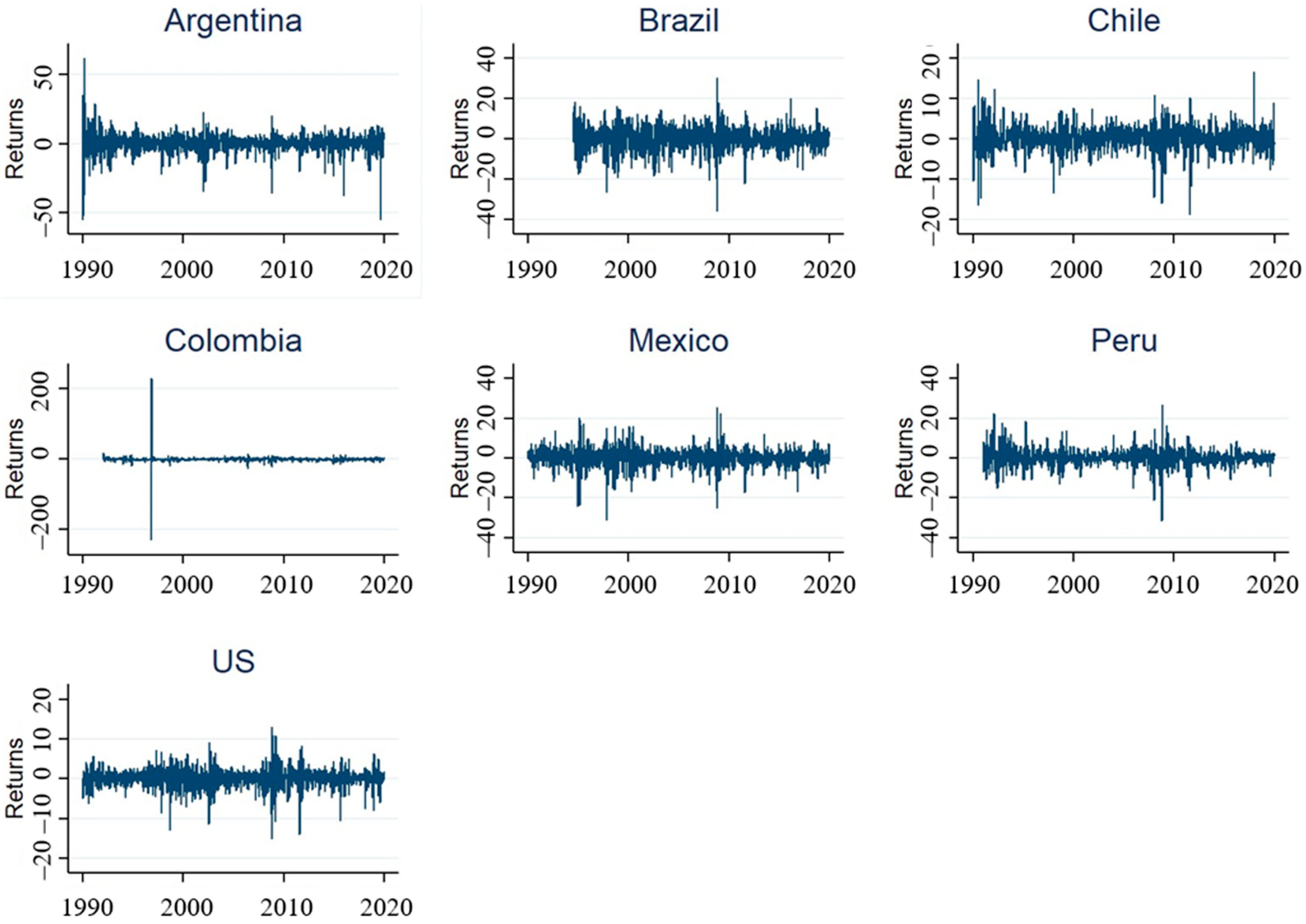
Utilities	−0.086	0.058	0.007	0.055	0.155	0.035	0.864	0.240	0.108	0.041	0.092	0.029	0.084	0.022

presents the summary statistics for every country sorted by industry. The summary statistics show huge variations in returns. Returns range from −25.80% to 86.40%. Also, the volatility of the market in terms of standard deviation of all indices is relatively high during the sample period. Standard deviations range from about 2.20% to 24.01%. In our sample, Colombia is the most vulnerable in terms of returns and standard deviations: it exhibits the highest and lowest returns, and the highest standard deviations among countries. Compared to other countries, the US exhibits the lowest standard deviations and the second highest returns, which show the ideal market conditions.

Figure 1 shows a graphical representation of the returns on the main market indices for each country. A visual representation shows that the market indices for these countries are stationary.6 In addition, we generate normality and autocorrelation tests for further analysis.7

Billio et al. (2015) show that unconditional correlations performed as well as more sophisticated financial integration measures proposed in the existing literature and, even though many authors have shown that correlation is time varying, the unconditional correlation of each country’s main market and sectors indices to determine each country’s pairwise correlation without considering the time-variance adjustments. This way one can establish if the correlations have drastically changed during the different time periods.

Table 2. Unconditional correlations of main market indices and sectors. Table 2 reports unconditional correlations of main market indices and sectors. When we report unconditional correlations of energy and real estate sectors, we exclude Mexico and Colombia, respectively, due to data unavailability. The sample data period is between 1 January 1990 and 31 December 2019.

Main Market Index	Argentina	Brazil	Chile	Colombia	Mexico	Peru	US
Argentina	1.000
Brazil	0.538	1.000
Chile	0.468	0.598	1.000
Colombia	0.109	0.133	0.168	1.000
Mexico	0.508	0.649	0.536	0.142	1.000
Peru	0.403	0.514	0.526	0.162	0.472	1.000
US	0.432	0.574	0.498	0.156	0.617	0.408	1.000
Basic Materials	Argentina	Brazil	Chile	Colombia	Mexico	Peru	US
Argentina	1.000
Brazil	0.365	1.000
Chile	0.322	0.559	1.000
Colombia	0.063	0.108	0.133	1.000
Mexico	0.362	0.629	0.477	0.111	1.000
Peru	0.219	0.416	0.370	0.092	0.444	1.000
US	0.333	0.640	0.503	0.112	0.605	0.394	1.000
Consumer Discretionary	Argentina	Brazil	Chile	Colombia	Mexico	Peru	US
Argentina	1.000
Brazil	0.275	1.000
Chile	0.223	0.395	1.000
Colombia	0.046	0.092	0.059	1.000
Mexico	0.301	0.437	0.372	0.075	1.000
Peru	0.020	0.052	0.022	0.029	0.032	1.000
US	0.225	0.347	0.393	0.076	0.507	0.030	1.000
Consumer Staples	Argentina	Brazil	Chile	Colombia	Mexico	Peru	US
Argentina	1.000
Brazil	0.326	1.000
Chile	0.307	0.370	1.000
Colombia	0.047	0.122	0.143	1.000
Mexico	0.303	0.303	0.269	0.110	1.000
Peru	0.108	0.149	0.147	0.006	0.107	1.000
US	0.233	0.302	0.305	0.123	0.270	0.072	1.000
Energy	Argentina	Brazil	Chile	Colombia	Peru	US
Argentina	1.000
Brazil	0.391	1.000
Chile	0.300	0.480	1.000
Colombia	0.294	0.530	0.431	1.000
Peru	0.159	0.296	0.279	0.302	1.000
US	0.417	0.667	0.507	0.528	0.334	1.000
Financials	Argentina	Brazil	Chile	Colombia	Mexico	Peru	US
Argentina	1.000
Brazil	0.323	1.000
Chile	0.332	0.532	1.000
Colombia	0.239	0.451	0.482	1.000
Mexico	0.284	0.525	0.505	0.422	1.000
Peru	0.191	0.303	0.328	0.304	0.258	1.000
US	0.267	0.465	0.442	0.369	0.490	0.222	1.000
Industrials	Argentina	Brazil	Chile	Colombia	Mexico	Peru	US
Argentina	1.000
Brazil	0.261	1.000
Chile	0.244	0.424	1.000
Colombia	0.158	0.332	0.251	1.000
Mexico	0.239	0.559	0.430	0.330	1.000
Peru	0.040	0.075	0.092	0.060	0.100	1.000
US	0.208	0.511	0.396	0.293	0.597	0.124	1.000
Real Estate	Argentina	Brazil	Chile	Mexico	Peru	US
Argentina	1.000
Brazil	0.294	1.000
Chile	0.150	0.385	1.000
Mexico	0.202	0.422	0.391	1.000
Peru	0.104	0.110	0.081	0.145	1.000
US	0.196	0.423	0.430	0.430	0.119	1.000
Telecommunications	Argentina	Brazil	Chile	Colombia	Mexico	Peru	US
Argentina	1.000
Brazil	0.371	1.000
Chile	0.252	0.385	1.000
Colombia	0.753	0.254	0.222	1.000
Mexico	0.327	0.606	0.398	0.302	1.000
Peru	0.090	0.136	0.080	0.028	0.123	1.000
US	0.262	0.486	0.293	0.238	0.537	0.084	1.000
Utilities	Argentina	Brazil	Chile	Colombia	Mexico	Peru	US
Argentina	1.000
Brazil	0.219	1.000
Chile	0.271	0.491	1.000
Colombia	0.110	0.451	0.472	1.000
Mexico	0.120	0.339	0.386	0.390	1.000
Peru	0.092	0.254	0.143	0.170	0.148	1.000
US	0.037	0.304	0.238	0.231	0.244	0.081	1.000

shows the correlations among the examined indices. At a first glance, we observe that there are no negative correlations, which indicates that these countries up to a given extent move in the same direction. For the main market index, the highest correlations are between Brazil and Mexico with 0.649, the US and Mexico with 0.617. Also, Brazil and the US with 0.574, and Brazil and Argentina with 0.538 exhibit strong positive correlations as well.

In addition, we report correlations between all countries sorted by industry.8 We observe all correlations are positive and each country and industry exhibit different levels of connectedness. For example, the basic materials sector the highest correlation is between the US and Brazil with 0.640; for consumer services, the US and Mexico share the strongest relation with 0.507, while for consumer goods, the strongest pairwise correlation is between Chile and Brazil with 0.370. Brazil dominates the energy (and utilities) correlation with the US (and Chile) with correlations of 0.667 (and 0.491). Mexico dominates the correlation with the US in the industrials sector with 0.597.

Now that we have a sense of the pairwise correlations among the countries and their sectors, the univariate generalized autoregressive conditional heteroskedasticity (GARCH) model is considered since all the returns showed autocorrelation. The next step included the estimation of the univariate GARCH model and selecting the best model based on the Akaike Information Criterion (AIC) and Schwarz’s Bayesian Criterion (BIC) to determine the best GARCH model based on the estimation of each model. As previously stated, the best model was selected among the traditional GARCH, EGARCH, GJR-GARCH and TGARCH. The model with the lowest AIC (BIC) score will be selected since it shows the best fit.

According to the results in

Table 3. Univariate GARCH Models. Table 3 reports traditional GARCH, EGARCH, GJR-GARCH, and TGARCH models and their parameters sorted by industry. The sample data period is between 1 January 1990 and 31 December 2019.

Argentina	Model Selected	ω	θ	Z	δ
Main Index	EGARCH	0.219 ***	−0.068 ***	0.263 ***	0.941 ***
Basic Materials	GARCH	1.351 ***	0.130 ***	N/A	0.843 ***
Consumer Discretionary	EGARCH	0.256 ***	0.019 *	0.355 ***	0.942 ***
Consumer Goods	GJR-GARCH	1.861 ***	0.162 ***	0.087 ***	0.758 ***
Energy	EGARCH	0.273 ***	−0.061 ***	0.326 ***	0.930 ***
Financial	EGARCH	0.140 ***	−0.021 ***	0.232 ***	0.965 ***
Industrials	EGARCH	0.154 ***	−0.150 *	0.352 ***	0.963 ***
Real Estate	GJR-GARCH	1.436 ***	0.106 ***	−0.052 ***	0.869 ***
Telecommunications	EGARCH	0.432 ***	−0.098 ***	0.250 ***	0.885 ***
Utilities	GJR-GARCH	0.565 ***	0.086 ***	0.065 ***	0.880 ***
Brazil	Model Selected	ω	θ	Z	δ
Main Index	EGARCH	0.145 ***	−0.075 ***	0.174 ***	0.958 ***
Basic Materials	EGARCH	0.102 ***	−0.063 ***	0.198 ***	0.970 ***
Consumer Discretionary	EGACRH	0.227 ***	−0.065 ***	0.178 ***	0.929 ***
Consumer Goods	GJR-GARCH	0.856 ***	0.144 ***	−0.010 ***	0.839 ***
Energy	EGARCH	0.205 ***	−0.061 ***	0.180 ***	0.946 ***
Financial	GJR-GARCH	26.370 ***	0.352 ***	−0.327 ***	−0.093 **
Industrials	GJR-GARCH	1.082 ***	0.126 ***	−0.076 ***	0.861 ***
Real Estate	EGACRH	0.084 ***	−0.056 ***	0.139 ***	0.976 ***
Telecommunications	EGARCH	0.147 ***	−0.064 ***	0.183 ***	0.955 ***
Utilities	EGARCH	0.084 ***	−0.056 ***	0.139 ***	0.976 ***
Chile	Model Selected	ω	θ	Z	δ
Main Index	GJR-GARCH	1.632 ***	0.220 ***	0.023 ***	N/A
Basic Materials	GJR-GARCH	0.389 ***	0.111 ***	−0.035 ***	0.880 ***
Consumer Discretionary	GARCH	3.285 ***	0.156 ***	N/A	0.651 **
Consumer Goods	GJR-GARCH	0.199 ***	0.115 ***	−0.047 ***	0.897 ***
Energy	GJR-GARCH	1.130 ***	0.117 ***	−0.059 ***	0.843 ***
Financial	GJR-GARCH	0.302 ***	0.137 ***	−0.091 ***	0.890 ***
Industrials	GJR-GARCH	0.268 ***	0.135 ***	−0.045 ***	0.877 ***
Real Estate	EGARCH	0.196 ***	−0.028 **	0.221 ***	0.937 ***
Telecommunications	GJR-GARCH	0.429 ***	0.098 ***	−0.037 ***	0.902 ***
Utilities	EGARCH	0.112 ***	−0.044 ***	0.212 ***	0.954 ***
Colombia	Model Selected	ω	θ	Z	δ
Main Index	GARCH	49.422 ***	0.072 ***	N/A	−0.008 *
Basic Materials	GARCH	−0.108 ***	−0.001 ***	N/A	1.000 ***
Consumer Discretionary	GARCH	0.014 ***	−0.002 ***	N/A	1.003 **
Consumer Goods	TGARCH	−0.008 ***	−0.005 ***	N/A	1.000 ***
Energy	EGARCH	3.607 ***	0.851 ***	1.251 ***	0.168 ***
Financial	EGARCH	0.477 ***	−0.271 ***	−0.148 ***	0.856 ***
Industrials	EGARCH	0.068 ***	−0.045 ***	0.200 ***	0.982 ***
Telecommunications	GJR-GARCH	11.067 ***	0.175 ***	0.212 ***	0.383 ***
Utilities	GARCH	0.010 ***	−0.001 ***	N/A	0.999 ***
Mexico	Model Selected	ω	θ	Z	δ
Main Index	EGARCH	0.167 ***	−0.113 ***	0.220 ***	0.943 ***
Basic Materials	GJR-GARCH	1.108 ***	0.128 ***	−0.063 ***	0.854 ***
Consumer Discretionary	EGARCH	0.127 ***	−0.071 ***	0.216 ***	0.955 ***
Consumer Goods	EGARCH	0.210 ***	−0.173 ***	0.328 ***	0.942 ***
Financial	EGARCH	0.110 ***	−0.096 ***	0.213 ***	0.966 ***
Industrials	EGARCH	0.208 ***	−0.096 ***	0.198 ***	0.934 ***
Real Estate	GARCH	2.180 ***	0.088 ***	N/A	0.726 ***
Telecommunications	EGARCH	0.169 ***	−0.084 ***	0.198 ***	0.947 ***
Utilities	TGARCH	N/A	N/A	N/A	N/A
Peru	Model Selected	ω	θ	Z	δ
Main Index	GJR-GARCH	0.630 ***	0.147 ***	0.044 ***	0.799 ***
Basic Materials	EGARCH	0.113 ***	−0.048 ***	0.214 ***	0.959 ***
Consumer Discretionary	GARCH	0.213 ***	0.025 ***	N/A	0.970 ***
Consumer Goods	GARCH	0.014 ***	0.083 ***	N/A	0.935 ***
Energy	GARCH	26.500 ***	0.198 ***	N/A	0.257 ***
Financial	EGARCH	0.116 ***	0.003 ***	0.364 ***	0.944 ***
Industrials	EGARCH	5.186 ***	0.317 ***	−0.021 ***	−0.149 ***
Real Estate	EGARCH	0.021 ***	−0.047 ***	0.074 ***	0.997 ***
Telecommunications	GARCH	3.557 ***	0.337 ***	N/A	0.703 ***
Utilities	GJR-GARCH	0.224 ***	0.095 ***	−0.062 ***	0.906 ***
US	Model Selected	ω	θ	Z	δ
Main Index	EGARCH	0.117 ***	−0.163 ***	0.236 ***	0.924 ***
Basic Materials	GJR-GARCH	0.317 ***	0.130 ***	−0.087 ***	0.880 ***
Consumer Discretionary	EGARCH	0.132 ***	−0.156 ***	0.260 ***	0.917 ***
Consumer Goods	EGARCH	0.086 ***	−0.126 ***	0.201 ***	0.935 ***
Energy	EGARCH	0.111 ***	−0.099 ***	0.201 ***	0.950 ***
Financial	GJR-GARCH	0.282 ***	0.179 ***	−0.126 ***	0.847 ***
Industrials	EGARCH	0.108 ***	−0.139 ***	0.183 ***	0.942 ***
Real Estate	GJR-GARCH	0.334 ***	0.192 ***	−0.123 ***	0.825 ***
Telecommunications	GJR-GARCH	0.149 ***	0.098 ***	−0.089 ***	0.920 ***
Utilities	EGARCH	0.076 ***	−0.041 ***	0.254 ***	0.952 ***

Notes: *, **, and *** indicate a significance at the 10%, 5%, and 1% levels, respectively.

, GARCH (1,1) is the best model for 11 of the analyzed sectors’ returns. EGARCH (1,1) and GJR-GARCH (1,1) are present in 34 and 21 of studied sectors, respectively. Like EGARCH (1,1) and GJR-GARCH (1,1), TGARCH (1,1) also shows the presence of asymmetric effects on these sectors. This indicates that there exist significant asymmetric effects on time series. For example, the EGARCH (1,1) model predominates in Argentina, Brazil, Mexico, and the US. Also, GJR-GARCH (1,1) predominates within sectors, indicating that most countries and sectors react differently to good and/or bad news. Before moving to the conditional correlation approach, we generate normality tests for the residuals and the squared residuals of the models.9

As previously stated, the DCC-GARCH model will be a bivariate model, with the US market and US sectors being paired with their respective counterpart from the Latin American countries (Argentina, Brazil, Chile, Colombia, Mexico, and Peru). That is, the US will be paired with each Latin American country’s index to determine their comovement. The estimates of the dynamics on the conditional correlations are shown in

Table 4. DCC GARCH Model—US and Latin American Countries. Table 4 reports the estimates of the DCC-GARCH model. In all six tables, the US will be paired with each Latin American country’s index to determine their comovement.

Argentina and US	a	b	Brazil and US	a	b
Market Index	0.032 **	0.941 ***	Market Index	0.069	0.923 ***
Basic Materials	0.031 **	0.948 ***	Basic Materials	0.067 ***	0.931 ***
Consumer Discretionary	0.053 **	0.829 ***	Consumer Discretionary	0.018 ***	0.981 ***
Consumer Goods	0.023 *	0.946 ***	Consumer Goods	0.043 **	0.847 ***
Energy	0.029 ***	0.949 ***	Energy	0.072 ***	0.918 ***
Financials	0.029	0.925 ***	Financials	0.029 **	0.975 ***
Industrials	0.007	0.971 ***	Industrials	0.063 ***	0.935 ***
Real Estate	0.024 **	0.958 ***	Real Estate	0.047 *	0.880 ***
Telecommunications	0.029 ***	0.937 ***	Telecommunications	0.053 **	0.904 ***
Utilities	0.021 *	0.948 ***	Utilities	0.035 ***	0.955 ***
Peru and US	a	b	Chile and US	a	b
Market Index	0.035	0.914 **	Market Index	0.034 **	0.952 ***
Basic Materials	0.033 *	0.966 ***	Basic Materials	0.054 ***	0.944 ***
Consumer Discretionary	0.027 **	0.965 ***	Consumer Discretionary	0.017 ***	0.977 ***
Consumer Goods	0.009	0.126	Consumer Goods	0.047 ***	0.921 ***
Energy	0.038 *	0.911 ***	Energy	0.044 *	0.946 ***
Financials	0.019 **	0.978 ***	Financials	0.059 ***	0.927 **
Industrials	0.01	0.967 ***	Industrials	0.049 ***	0.945 ***
Real Estate	0	0.991 ***	Real Estate	0.012 *	0.984 ***
Telecommunications	0.001	0.994 ***	Telecommunications	0.037	0.527 **
Utilities	0.003	0.986 ***	Utilities	0.029 ***	0.958 ***
Colombia and US	a	b	Mexico and US	a	b
Market Index	0.015 ***	0.980 ***	Market Index	0.050 ***	0.947 ***
Basic Materials	0.696 ***	0.035	Basic Materials	0.058 ***	0.938 ***
Consumer Discretionary	0.008	0.994 ***	Consumer Discretionary	0.044	0.934 ***
Consumer Goods	0.195	0.520 **	Consumer Goods	0.067 *	0.918 ***
Energy	0.033 **	0.964 ***	Financials	0.062 ***	0.878 **
Financials	0.265 **	0.114	Industrials	0.064 ***	0.935 ***
Industrials	0.053 **	0.917 ***	Real Estate	0.098 **	0.856 ***
Telecommunications	0.142 **	0.189	Telecommunications	0.043 ***	0.941 ***
Utilities	0.011 *	0.975 ***	Utilities	0.005	0.982 ***

Notes: *, **, and *** indicate a significance at the 10%, 5%, and 1% levels, respectively.

. The coefficients among the different sectors and countries are quite similar. We observe that coefficients $a$ are relatively small (with the except of a couple of the coefficients), indicating that conditional volatility does not change very rapidly. Coefficients $b$ are much larger than coefficients $a$, indicating gradual fluctuations over time. We confirm that the estimated coefficients $a$ and $b$ satisfy the stationary conditions for all the variance and covariance processes.

Table 5. Summary statistics of bivariate conditional correlation. Table 5 reports the summary statistics of bivariate conditional correlation. In Table 5, we only report the main market index.

Country List	Mean	Median	Min	Max	SD
Argentina and US	0.382	0.380	−0.001	0.741	0.126
Brazil and US	0.514	0.528	−0.075	0.870	0.189
Chile and US	0.377	0.400	−0.029	0.669	0.146
Colombia and US	0.182	0.189	−0.069	0.424	0.126
Mexico and US	0.532	0.588	−0.124	0.861	0.213
Peru and US	0.267	0.273	−0.057	0.644	0.093

presents the summary statistics of the bivariate conditional correlations between the US and each of the respective Latin American markets. It is important to notice that similar to the unconditional correlations, we find that all the Latin American indices studied have an average positive correlation with the US indices. In terms of the market index, on average, Mexico has the highest conditional correlation with the US with 0.532, and Colombia has the lowest mean conditional correlation relative to the US with 0.182, indicating that Mexican market tends to comove with US markets relatively more compared to the remaining Latin American countries. This is not surprising since Mexico has engaged in a free trade agreement with the US since 1994. Also, the geographical proximity to the US is significant for their strong comovement. On the other hand, Colombia has the lowest conditional correlation, which should imply higher diversification gains to an American investor relative to the rest of Latin America nations. Moreover, the ranking shows that the more developed countries (Argentina, Brazil, and Mexico) within this group have a higher positive dynamic conditional correlation with the US than the relatively less developed countries (Colombia and Peru). Lastly, we observe that more developed countries (Argentina, Brazil, and Mexico) tend to have a higher correlation with the US than relatively less developed countries (Colombia and Peru). These findings show where American investors can get portfolio diversification benefits with Latin American countries and their sectors as well.10

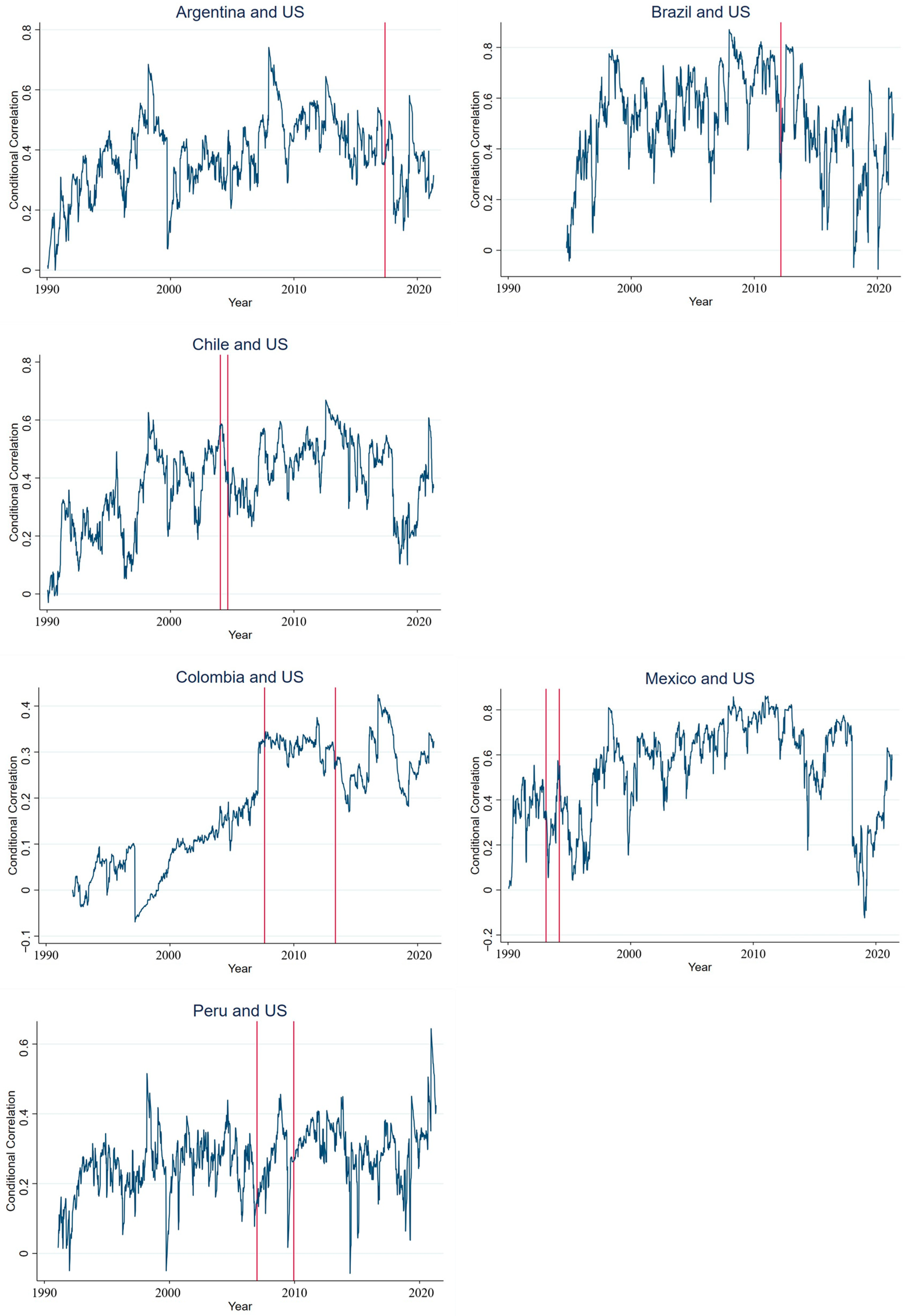
The dynamic conditional correlation for the main market indices between the US and the examined countries can be seen in Figure 2. All graphs show two lines that denote the signing date of the trade agreement with the US, while the second line shows the point in time in which the trade deal started and was implemented. A visual examination of the Argentina–US conditional correlation shows that conditional correlation has increased from the start of the sample (1990) and mostly increased through time. Some of the abrupt changes can be attributed to the several financial problems related to currency issues as well as default problems that Argentina has encountered in the last 15 years. Brazil has a very low correlation and large spikes on the beginning of the sample, which coincide with the implementation of the Real as the nation’s currency (replacing the cruzeiro real). However, we observe an upward trend and a significant increase in correlations, especially during the financial crisis and the years after that. For Chile, we observe that comovement was low at the beginning of the sample but gradually increased while the country started liberalizing its market. Colombia shows a low correlation with the US for the first 10 years but has a significant bump in correlation close to the signing of the bilateral free trade agreement with the US. After that considerable rise, the correlations seem to stabilize during the new range. In 2016, Colombia experienced high inflation and lowered GDP growth. This matches the movements shown in the graph of the dynamic conditional correlation. Mexico shows a different story than the rest of the countries. It seems that comovement between the US and Mexico has been significantly strong over most of the sample. However, the later part of the sample correlation between these countries suffers a significant downward trend for a short period. Although it does not involve any specific crisis or country specific turmoil, it does conform with the initial stages of negotiation of a new trade agreement. During this time, several negotiation talks failed to move the new agreement forward and talks of eliminating free trade between Mexico and the US were surfaced. After long negotiations occurred, a new deal was signed, and the graphs shows the correlation bouncing back to previous values. Lastly, Peru has been a relatively small market in Latin America that has started growing in the last 10 years. The graph of the conditional correlation shows that comovement was relatively low and has a gradual trend towards a higher degree of comovement. The graphs for the remaining sector indices show similar effects to the ones shown on the main market indices.

4.2. Smooth Transition Model

The smooth transition model on the dynamic bivariate conditional correlation between the US and the examined Latin American countries was computed.11

The results of the smooth transition estimation are shown in

Table 6. The estimated smooth transition model. Table 6 presents the smooth transition model to estimate the average correlation between two different regimes.

Argentina and US	α	β	γ	T	Midpoint
Market Index	0.378 ***	0.094 *	633 ***	0.449 ***	Jun-03
Basic Materials	0.293 ***	0.008	242 ***	0.292 ***	Sep-98
Consumer Discretionary	0.193 ***	−0.084 *	13.300	0.566 ***	Dec-06
Consumer Goods	0.240 ***	0.011 *	316.00	0.223 ***	Oct-96
Energy	0.341 ***	−0.024 ***	581 ***	0.467 ***	Jan-04
Financials	0.317 ***	−0.010 *	434 **	0.325 ***	Oct-99
Industrials	0.262 ***	−0.095	31.8 **	0.476 ***	Apr-04
Real Estate	0.222 ***	0.244 ***	4.13 ***	0.584 ***	Jul-07
Telecommunications	0.246 ***	0.417	7.77 **	0.889 *	Aug-16
Utilities	0.183 ***	0.018 ***	66.3 ***	0.228 ***	Oct-96
Brazil and US	α	β	γ	T	Midpoint
Market Index	0.513 ***	−0.064 **	1116 ***	0.554 ***	Jan-04
Basic Materials	0.536 ***	−0.010 **	786 ***	0.656 ***	Aug-09
Consumer Discretionary	0.318 ***	−0.624	111 **	0.682 ***	Jun-10
Consumer Goods	0.277**	0.055	76.70	0.152 ***	May-95
Energy	0.492 ***	−0.006 **	506	0.523 ***	Sep-05
Financials	0.339 ***	−0.015	98	0.272 ***	Mar-95
Industrials	0.402 ***	−0.014 **	582	0.371 ***	Feb-01
Real Estate	0.323 ***	−0.077 *	227	0.484 ***	Apr-99
Telecommunications	0.374 ***	−0.018 *	21.9 ***	0.305 ***	Feb-99
Utilities	0.184 ***	0.114 ***	355 ***	0.052 ***	Jul-91
Chile and US	α	β	γ	T	Midpoint
Market Index	0.358 ***	0.024	51.3 ***	0.262 ***	Nov-97
Basic Materials	0.04	0.348 ***	116 ***	0.142 ***	Mar-94
Consumer Discretionary	0.239 ***	0.099 **	149 ***	0.019 ***	Aug-90
Consumer Goods	0.254 ***	0.523 ***	12.3 ***	0.780 ***	May-13
Energy	0.199 ***	0.060 ***	125 ***	0.025 ***	Oct-90
Financials	0.250 ***	0.055	13.2 ***	0.137 *	Jan-94
Industrials	−0.059	0.319 ***	434 ***	0.173 ***	Apr-95
Real Estate	0.140 ***	0.015 ***	377 ***	0.081 ***	May-92
Telecommunications	0.247 ***	−0.009 ***	99.3 ***	0.142 ***	Apr-94
Utilities	0.198 ***	0.042 ***	6.90 ***	0.065 *	Dec-91
Colombia and US	α	β	γ	T	Midpoint
Market Index	0.080 ***	0.166 **	21.2 ***	0.211 *	Dec-95
Basic Materials	0.049 **	−0.739 ***	8.62 ***	0.805 ***	Feb-14
Consumer Discretionary	0.014 *	0.069 ***	21.9 ***	0.006	Sep-91
Consumer Goods	0.120 ***	−0.034 ***	213 ***	0.265 ***	Dec-97
Energy	0.175 ***	0.029 *	674 ***	0.119 **	Jul-93
Financials	0.108 ***	−0.379**	19 ***	0.797 ***	Nov-13
Industrials	0.292 ***	0.004 *	812 ***	0.241 ***	Mar-97
Telecommunications	0.226 ***	0.071 ***	26.0 ***	0.506 ***	Jan-05
Utilities	0.115 ***	0.216	9.14 ***	0.508 ***	Mar-05
Mexico and US	α	β	γ	T	Midpoint
Market Index	0.512 ***	0.122 *	277 ***	0.375 ***	Mar-01
Basic Materials	0.348 ***	0.144 ***	151 **	0.161 **	Oct-94
Consumer Discretionary	0.376 ***	0.051	63	0.224 ***	Sep-96
Consumer Goods	0.157 ***	0.131 ***	502 ***	0.040 ***	Mar-91
Financials	0.261 ***	0.08	417 ***	0.045 ***	Apr-91
Industrials	−0.152	0.622 ***	95 ***	0.119 ***	Jul-93
Real Estate	0.334 ***	0.057 **	37.2 ***	0.211 ***	Apr-96
Telecommunications	0.349 ***	0.040 **	39.9 ***	0.298 ***	Nov-98
Utilities	0.192 ***	−0.344	15.8 **	0.422 *	Aug-02
Peru and US	α	β	γ	T	Midpoint
Market Index	0.261 ***	0.213 **	65.5 ***	0.303 ***	Feb-99
Basic Materials	0.276 ***	0.099 ***	4.55 **	0.328 **	Jul-98
Consumer Discretionary	0.219 ***	−0.139 **	255 ***	0.114 ***	May-93
Consumer Goods	0.102 ***	0.012 ***	84.2 ***	0.235 ***	Jan-97
Energy	0.259 ***	0.034	254 ***	0.249 ***	Jul-96
Financials	0.142 ***	0.066 ***	12.5 ***	0.471 ***	Feb-04
Industrials	0.144 ***	0.495 ***	13.3 ***	0.552 ***	Jul-06
Real Estate	0.052 ***	0.002	681 ***	0.102 **	Dec-91
Telecommunications	0.074 ***	0.016	516 ***	0.086 ***	May-92
Utilities	0.109 ***	0.318	6.69 ***	0.776	Apr-14

Notes: *, **, and *** indicate a significance at the 10%, 5%, and 1% levels, respectively.

. The smooth transition model estimates the average correlation between two different regimes. The term $\alpha$ is the average correlation of the first (old) regime, while $\beta$ is the change in correlation of the second (new) regime. Consequently, $\alpha +\beta$ is an indicator of the average correlation of the second (new) regime. The term γ establishes the slope of the transition curve. The higher the values of $\gamma$, the more drastic the change between the two correlations (old and new) regimes. Lastly, $\tau$ shows the midpoint or turning point of the transition curve.

For the market index comovement between the US and Argentina, the first regime has an average correlation of 0.378, while the second regime has correlation of 0.472. This would be clear evidence that comovement has increased during the sample period. The midpoint was in mid-2003, and it shows a large γ, which signifies a more abrupt change in correlations. On the other hand, Brazil shows an average correlation of 0.513 on the first part of the sample, but the second regime reduces by 0.064, resulting in a decrease in comovement in the second regime. The market index in Chile shows a 0.358 correlation for the first regime and a 0.024 correlation for the second regime. For Colombia, the midpoint was in the earliest part of the sample in late 1995. The correlation regimes moved from 0.080 to 0.246. Mexico also shows a similar story with an old regime correlation of 0.512 and with a new correlation regime of 0.634. In this case, the midpoint occurred in early 2001. Peru shows an old regime correlation of 0.261 and a new correlation regime of 0.474, which is the biggest increase in correlation among the main market indices. From all the countries’ main indices, all increased their level of comovement with the US in the smooth transition approach except Brazil. We conclude that the degree of comovement mostly increased. In terms of all the different sectors across the Latin American countries, the results show that the majority of the indices exhibit an increase in correlation from the old regime to the new one, indicating that different countries and sectors have shifted differently over the entire sample, but most of the countries show a significant increase.

Employing the smooth transition model, we observe that the comovement between the US and Latin American countries (except Brazil) has increased during the sample period. One downside of this model is that we only consider one midpoint of the entire sample of 30 years. To check robustness of the smooth transition model, we generate tests for a unit root on the residuals of the model.12 We confirm that the smooth transition model is appropriate for the evaluated series.

4.3. Structural Breaks

The structural break analysis was divided into two main approaches. The first included testing known dates that includes considering if structural breaks are present during the signing date as well as during the established start date of the bilateral trade agreements. The second approach tested for unknown structural breaks. In

Table 7. Structure breaks and regression analysis. In Table 7, we report structural breaks with known dates (Panel A) and unknow dates (Panel B). Also, the regression analysis was taken to examine directly if the dynamic conditional correlation between these countries has changed after the signing and implementation of each trade agreement (Panel C).

Panel A. Structure Breaks—Known Dates
Country List	Sign Date	Start Date
Argentina and US	3.737	3.737
Brazil and US	3.841	3.841
Chile and US	5.621 *	2.841
Colombia and US	5.833 **	3.353
Mexico and US	6.602 **	7.204 **
Peru and US	6.577 **	6.920 **
Panel B. Structure Breaks—Unknown Dates
Country List	Number of Breakpoints	Estimated Break Dates
Argentina and US	5	07-1994; 04-1999; 05-2006; 01-2011; 04-2016
Brazil and US	5	04-1998; 07-2002; 05-2006; 02-2011; 03-2016
Chile and US	5	01-1997; 06-2003; 05-2006; 11-2010; 07-2015
Colombia and US	5	12-1997; 03-2002; 08-2006; 02-2011; 04-2015
Mexico and US	5	07-1996; 05-2011; 05-2006; 01-2011; 07-2015
Peru and US	5	07-1997; 07-2002; 04-2006; 05-2011; 08-2015
Panel C. Regression Analysis
Country List	Sign Date	Start Date
Argentina and US	0.051 ***	0.051 ***
Brazil and US	−0.122 ***	−0.122 ***
Chile and US	0.118 ***	0.115 ***
Colombia and US	0.212 ***	0.135 ***
Mexico and US	0.202 ***	0.225 ***
Peru and US	0.060 ***	0.065 ***

Notes: *, **, and *** indicate a significance at the 10%, 5%, and 1% levels, respectively.

Panel A, we report results for the structural breaks around the signing and start dates of the dynamic conditional correlations, showing the presence of structural breaks in some of the main indices.

We observe structural breaks for Chile, Colombia, Mexico, and Peru, while the other two (Argentina and Brazil) do not exhibit a structural break after the signing or start dates of their trade agreements. This coincides with the countries that have a stronger trade agreement with the US. It is important to recall that Colombia, Chile, Mexico, and Peru have a full bilateral free trade agreement, while Argentina and Brazil have trade agreements that are not completely free trade agreements, hence their strength is weaker relative to a full free trade agreement. Some specific sectors such as materials, consumer goods, financial, energy, and industrial exhibit the highest number of structural breaks during the sign and start dates, indicating that such industries in Latin America tend to have a higher level of commercial connection with the US.13

In addition, we report unknown structure breaks in Table 7 Panel B. Contrary to the known structural breaks, the unknown structural break approach used by Bai and Perron (2003) tests for a specified number of breaks in the bivariate dynamic conditional correlation. In this case, the unknown structural breaks were limited to five but would incorporate more than five if these breaks were present. The results of the unknown structural breaks show a very similar story to the one from the known structural breaks (signing and start dates). It is also important to consider that several unknown breaks are very close to the signing and start dates. Although the structural breaks are not on the exact same date, according to the data, there is a break present near that specific date. This can be attributed to the trade agreements considering there are significant or major events that could produce such a shock on the correlation between these countries in that given time. As mentioned previously and as shown by the analysis, the impact on the bivariate dynamic conditional correlation might not be shown immediately but over a more prolonged period of time. Therefore, the smooth transition model was considered to study how the correlations have changed over the sample period.

Lastly, to examine directly if the dynamic conditional correlation between these countries has changed after the signing and implementation of each trade agreement, a regression approach was taken. The idea is to use the dynamic conditional correlation as the dependent variable, and an indicator variable determines the creation and implementation of the trade agreements. In Table 7, Panel C presents the coefficients of the model, and we observe that after the respective bilateral trade agreements between the US and Argentina, Chile, Colombia, Mexico, and Peru have increased comovement in the main market indices between these countries. Also, the US and Brazil’s dynamic conditional correlation shows a negative and significant coefficient that signifies that the comovement between the US and Brazil has fallen after the implementation of their trade agreement.

5. Conclusions

The main objective of this study was to empirically investigate if the comovement between main stock indices of Argentina, Brazil, Colombia, Chile, Mexico, and Peru have shown greater or lower comovement in relation to the US financial markets. We conclude that main market indices of Argentina, Chile, Colombia, Mexico, and Peru have increased their correlation with the main market index in the US after the respective bilateral trade agreements. In addition, the results indicate that the integration with the US market index has increased over time for all the countries except for Brazil, which had a small reduction in correlation during the end of the sample period. The results of the smooth transition model also provide support for the previous claims.

The lower values and lack of structural breaks around Argentina and Brazil can be partly explained by the type of trade agreement. Considering that the agreements that Argentina and Brazil signed with the US are not full free trade agreements, the impact on financial market integration seems lower. On the contrary, the countries that do have a free trade agreement (Chile, Colombia, Mexico, and Peru) with the US have shown a higher number of structural breaks around the signing and implementation dates of these treaties. In addition, the regression-based approach shows the comovement between Latin American and the US financial markets.

The results show evidence that the financial market integration between these countries is varying consistently over time, so close attention must be taken. The implication of the study for policy makers can be stated as an increase in the level of correlations between Latin American and the US financial markets means that financial market disturbances in the US are more likely to be transmitted to these countries, which may have adverse consequences for the stability of the financial systems involved. On the other hand, a higher degree of comovement implies that optimal portfolios have changed as a result of the correlation variation; hence, investors will have to adjust their portfolios accordingly. The results support the idea that financial market integration in the region is increasing overall as well as the argument that the US has become more integrated with this region over time. Our main limitation is access to data for other Latin American countries. It will be beneficial to have further investigations including other Latin American countries for future research.

References

- Abbasov, Ahliman. 2019. Pooled Mean Group Approach to Test the Determinants of Financial Integration: Evidence From OECD and G20 Countries. Research in World Economy 3: 366–70. [Google Scholar] [CrossRef]
- Bae, Joon Woo, Redouane Elkamhi, and Mikhail Simutin. 2019. The best of both worlds: Accessing emerging economies via developed markets. Journal of Finance 74: 2579–617. [Google Scholar] [CrossRef]
- Bai, Jushan, and Pierre Perron. 2003. Computation and analysis of multiple structural change models. Journal of Applied Econometrics 18: 1–22. [Google Scholar] [CrossRef]
- Basnet, Hem C., and Subhash C. Sharma. 2013. Economic Integration in Latin America. Journal of Economic Integration 28: 551–79. [Google Scholar] [CrossRef]
- Bekaert, Geert, and Campbell R. Harvey. 1995. Time-varying world market integration. Journal of Finance 50: 403–44. [Google Scholar]
- Berben, Robert Paul, and W. Jos Jansen. 2005. Comovement in international equity markets: A sectoral view. Journal of International Money and Finance 24: 832–57. [Google Scholar] [CrossRef]
- Billio, Monica, Antonio Paradiso, Michael Donadelli, and Max Riedel. 2015. Measuring financial integration: Lessons from the correlation. University Ca’Foscari of Venice, Department of Economics Working Paper Series 2015: 23. [Google Scholar] [CrossRef]
- Bollerslev, Tim. 1986. Generalized autoregressive conditional heteroskedasticity. Journal of Econometrics 31: 307–27. [Google Scholar] [CrossRef]
- Chelley-Steeley, Patricia L. 2005. Modeling equity market integration using smooth transition analysis: A study of Eastern European stock markets. Journal of International Money and Finance 24: 818–31. [Google Scholar] [CrossRef]
- Didier, Tatiana, Ruth Llovet, and Sergio L. Schmukler. 2017. International financial integration of East Asia and Pacific. Journal of the Japanese and International Economies 44: 52–66. [Google Scholar] [CrossRef]
- Engle, Robert. 2002. Dynamic conditional correlation: A simple class of multivariate generalized autoregressive conditional heteroskedasticity models. Journal of Business & Economic Statistics 20: 339–50. [Google Scholar]
- Erkut, Burak, and Gagan Deep Sharma. 2023. Financial integration in Asia: New Empirical evidence using dynamic panel data estimations. International Economics and Economic Policy 20: 213–31. [Google Scholar] [CrossRef]
- Eun, Cheol S., and Sangdal Shim. 1989. International transmission of stock market movements. Journal of Financial and Quantitative Analysis 24: 241–56. [Google Scholar] [CrossRef]
- Forbes, Kristin J., and Menzie D. Chinn. 2004. A decomposition of global linkages in financial markets over time. Review of Economics and Statistics 86: 705–22. [Google Scholar] [CrossRef]
- Forbes, Kristin J., and Roberto Rigobon. 2002. No contagion, only interdependence: Measuring stock market comovements. Journal of Finance 57: 2223–61. [Google Scholar] [CrossRef]
- Fujii, Eiji. 2005. Intra and inter-regional causal linkages of emerging stock markets: Evidence from Asia and Latin America in and out of crises. Journal of International Financial Markets, Institutions and Money 15: 315–42. [Google Scholar] [CrossRef]
- Glosten, Lawrence R., Ravi Jagannathan, and David E. Runkle. 1993. On the relation between the expected value and the volatility of the nominal excess return on stocks. The Journal of Finance 48: 1779–801. [Google Scholar] [CrossRef]
- Johnson, Robert, and Luc Soenen. 2003. Economic integration and stock market comovement in the Americas. Journal of Multinational Financial Management 13: 85–100. [Google Scholar]
- Lim, Eun Son, and Janice Boucher Breuer. 2019. Free trade agreements and market integration: Evidence from South Korea. Journal of International Money and Finance 90: 241–56. [Google Scholar] [CrossRef]
- Lin, Chien Fu Jeff, and Timo Teräsvirta. 1994. Testing the constancy of regression parameters against continuous structural change. Journal of Econometrics 62: 211–28. [Google Scholar] [CrossRef]
- Longin, Francois, and Bruno Solnik. 1995. Is the correlation in international equity returns constant: 1960–1990? Journal of International Money and Finance 14: 3–26. [Google Scholar] [CrossRef]
- Nelson, Daniel B. 1991. Conditional heteroskedasticity in asset returns: A new approach. Econometrica: Journal of the Econometric Society 59: 347–70. [Google Scholar] [CrossRef]
- Rua, Antonio, and Luis C. Nunes. 2009. International comovement of stock market returns: A wavelet analysis. Journal of Empirical Finance 16: 632–39. [Google Scholar] [CrossRef]
- Shin, Kwanho, and Chan Hyun Sohn. 2006. Trade and financial integration in East Asia: Effects on co-movements. World Economy 29: 1649–69. [Google Scholar] [CrossRef]
- Vo, Xuan Vinh. 2022. Trade integration and international financial integration: Evidence from Asia. The Singapore Economic Review 67: 1275–86. [Google Scholar]
- Wang, Jun, Chengjuan Liao, Jie Xiong, and Chengbo Wang. 2023. Deepening of Free Trade Agreements and International Trade: Evidence from China. Emerging Markets Finance and Trade 59: 1960–75. [Google Scholar] [CrossRef]
- Zakoian, Jean Michel. 1994. Threshold heteroskedastic models. Journal of Economic Dynamics and Control 18: 931–55. [Google Scholar] [CrossRef]
Figure 1.
Returns of Latin American and the US market indices. Figure 1 presents returns of Latin American and the US market indices. This is based on weekly-based log returns sample data. The sample period is between 1 January 1990 and 31 December 2019.
Figure 2.
Conditional correlation of latin american market indices and the US market index returns. Figure 2 presents the dynamic conditional correlation for the main market indices between the US and the examined countries: Argentina, Brazil, Chile, Colombia, Mexico, and Peru. We also show (red) lines that denote the trade agreement signing date with the US. Two separate lines indicate that the signing date and implemented dates are different.