
The Current and Expected Pricing Markup as Derived from the Capital Asset Pricing Model and Tobin’s Q and Applied to the UK’s FTSE 100

Independent Researcher, London KT10 0EL, UK
J. Risk Financial Manag. 2024, 17(3), 127; https://doi.org/10.3390/jrfm17030127
Submission received: 19 February 2024
/
Revised: 14 March 2024
/
Accepted: 17 March 2024
/
Published: 20 March 2024
(This article belongs to the Section Economics and Finance)
Abstract
:Price markups and firms’ Tobin’s Q ratios are widely believed to have been increasing in the past several decades. Various models for the calculation of price markups have been developed, each relying on the historically held definition of the ratio of price to marginal cost; however, all of these have methodological drawbacks, and some of the results they have produced have been poorly reflective of the near past wider macroeconomic experience. This paper defines a new approach for the definition and measurement of markup pricing, and it also avoids some of the issues surrounding the marginal cost approaches by using the measure of economic rent and the capital asset pricing model. The results show limited markup pricing for the UK’s FTSE 100 companies (2018–2023), but that certain real estate, technology/media and financial services/equity investment firms have enjoyed higher price markup levels. An analysis of the business models of these firms is used to qualitatively propose explanations for such markups. This work offers formal proof that that the expected price markup is equal to Tobin’s Q and finds that the empiric market level of markup is near equivalent to the market Tobin’s Q; the differences between the markup and Tobin’s Q at the level of the firm are equally assessed. This work challenges the general consensus that price markups are above one and have been increasing; it may also aid policy makers with respect to taxation policy and regulatory measures, as well as the financial management of firms in decisions concerning capital deployment and portfolio management. The method merits expansion to wider data sets, as well as to those from outside of the UK.
1. Introduction
In conditions absent of perfect competition, a firm may achieve pricing in excess of marginal cost and thus enjoy monopoly rents through a price markup, where price markup is defined as the price divided by marginal cost (µ = P/MC). This can be demonstrated as a production level equilibrium point that produces deadweight loss and thus is societally inefficient. Higher price markups are equally believed to decrease the share to labour, and thus increases inequality, while reducing output and investment (inter alia De Loecker et al. 2020; Syverson 2019).
Starting in the 1950s, the structure–conduct–performance paradigm (SCPP) framework was used to estimate the measures of market power and price markup (Bain 1951). These studies attempted to regress structure, which was typically market concentration as measured by the Herfindahl–Hirschman index, with firm profits. This was achieved through investigating the hypothesis that high levels of concentration lead to market power. However, the approach has been largely abandoned in the face of criticism (see Bresnahan 1989). Structure will always likely be difficult to determine: What constitutes the market in which the firm operates? How might variation in a firm’s geographic footprint be accounted for? The black box of management conduct may represent a multiplicity of possibilities; furthermore, given prices and marginal costs are difficult or impossible to obtain, performance as based on those measures will be equally difficult to determine.
More recently, in the context of reported declines in the labour share (Elsby et al. 2013; Karabarbounis and Neiman 2014) as well as, more broadly, reports of rising inequality (Piketty 2014; Stiglitz 2015), the last few decades have seen the development of new approaches to the measurement of price markups. With the aforementioned problems of measuring marginal cost, these methods seek alternative estimates according to market transactions; however, these do not come without their own methodological challenges. These studies generally reported markup levels that rose over time and were all in excess of one.
In assuming cost minimisation and profit maximisation, production-function methods back out the markup given the production-function inputs, which should be employed to the point where the marginal returns of the inputs are equal to marginal costs. Hall (1988) determined the markup as the ratio of the output elasticity to a variable input and the share of the revenue paid to that input. The method assumes constant output elasticities. Moreover, in examining the changes in inputs to outputs over time, it is only able to offer a picture of the average markup over such long time frames. De Loecker and Eeckhout (2018) as well as De Loecker et al. (2020) further developed this production-function method employing a single production input only which does not require the calculation of profit. However, in assuming constant coefficients in the production function, the approach cannot account for technical change and requires a broad set of data and so makes for further technical difficulties. Crucially, marginal cost is assumed to be equal to average cost; thus, in an environment where fixed costs have outpaced variable costs, markups will be overestimated. We will examine in the ensuing discussion the strong possibility that this has indeed been the case over the studied period where there has been a growth in firm balance sheet intangibles, software, and R&D. This observation seems to be reflected in the results for these studies, which seem too high to be plausible: the reported global markup increasing from 1.15 in 1980 to 1.6 in 2016, and with the results for some countries (Denmark and Switzerland) more than doubling with markup levels approaching three. These estimates were greater than the rate required to explain the decline in the labour share, and they also failed to temporally match such labour share changes (Syverson 2019); the implied profit levels from such markups also did not translate into the reported firm profits during the period studied. Further, Raval (2023) has recently shown considerable differences in computed markups according to the input employed.1
Another approach by Barkai (2020), under the assumption of constant returns to scale, used the identity that the markup is equal to the ratio of revenue to total labour and capital costs. These costs were determined using US National Accounts data for labour compensation and the capital stock, with a user cost of capital to impute the cost of capital. The depreciation and inflation elements of the capital costs were not firm specific but rather limited to three categories; the cost of borrowing was similarly treated as the same across all firms. Furthermore, in using AAA bonds, the risk was set at a level that was highly likely to be lower than that faced by many firms. This study found an increase in economic profits from 2.2% (1984) to 15.7% in 2014.
More generally, such an emergence of high levels of markup is not reflective of the near past’s empiric macroeconomic environment (Basu 2019). If higher markups are not achieved through higher pricing (i.e., with ensuing inflation), then their source must be due to lower costs that are accrued from productivity gains; moreover, higher markups should be associated with lower employment given the output of the firm with market power will be lower than the firm in perfect competition. Instead, we have witnessed generally stable and near full employment, low inflation, and week productivity gains in the most recent past. We should also note that these approaches continue to rely on the ratio of price to marginal cost. This ignores any notion that the firm will have fixed costs, which, to be profitable, would need to be recovered through price. The historic definition of markup as the ratio of price to marginal cost remains problematic.
The most recent studies in the literature also point towards a contemporaneous increase in Tobin’s Q (Eggertsson et al. 2021). In a similar manner, we would expect a firm in perfect competition to have a Tobin’s Q of one. A market value that exceeds the replacement cost (i.e., Q > 1) signals anticipated future profit payments: economic rent. Under the condition of free market entry, we would imagine other firms entering the market and thus pushing the industry Q towards one as price competition takes hold. Lindenberg and Ross (1981) found a relationship between the price markup2 and Tobin’s Q, and Eggertsson et al. (2021) showed that ∂µ/∂Q > 0.
With no direct measure for marginal cost being available, these above-described studies have developed tremendously innovative approaches in extracting market transaction equivalents in order to estimate marginal costs. It must also be recognised that this body of literature points to a consensus that there has been, at least at some level, an increase in price markups with the associated increases in profits and a decline in the share to labour. What is clear is that there is no single model or data set that is likely to lead to a dispositive outcome: each has its own advantages and drawbacks. Further approaches are therefore needed to better develop the macroeconomic picture.
I propose an alternative approach for the calculation of the price markup, an approach that is most closely related to the economic-profit approach of Barkai (2020) and others (Caballero et al. 2017; Gutiérrez 2017). This approach avoids some of the problems that are encountered with the aforementioned methods, and it may also bridge the gap between reported markups and the wider macroeconomic experience. This paper aims to address the following: (1) to offer an alternative definition of price markups; (2) to compute price markups for the UK’s FTSE 100 companies (2018–2023); (3) to provide a theory for forward-looking price markups; (4) to explain variance in modelled markups to expected price markups; (5) to provide a microeconomic explanation where individual firm price markups appear significantly high and the markup diverges from the Tobin’s Q; and, (6) to offer implications for policy makers, and firm management.
2. Theory
2.1. Economic Rent and Price Markup
An accepted definition of economic rent is: ‘Those payments to a factor of production that are in excess of the minimum payment necessary to have that factor supplied’ (Varian 1987). I take the ‘payment’ as the firm’s income (Ii) and the ‘minimum payment necessary’ as the firm’s opportunity cost of equity (Ci).
Proposition 1.
The economic rent of the firm (Ei) is income minus the cost of equity.
Proposition 2.
The economic rent of the firm may be normalised according to revenue giving markup, µi.
where
PYi: revenue for firm i
Therefore, the markup for the market, µm, is:
where
Em: economic rent of the market
2.2. Expected Markup
Proposition 3.
The expected markup of the firm (µe) is equal to the firm’s current Tobin’s Q.
where Tobin’s Q is
where
µe = Q
M: market equity value of the firm
L: book value of liabilities of the firm
T: book equity of the firm
Proof.
µe = Q
M will be the sum of future economic rent (E) plus the cost of equity (C).
From financial terminal value theory, will be equal to Et.
Where
t: terminal coefficient for the firm
where
g: growth of the firm
c: cost of equity (%)
Now, is equal to , and given the terminal coefficient for the cost of equity will have g = 0, we have that t as applied to cT will be equal to . It follows that will be equal to T.
∴ M = Et + T
Let Q0 be the firm’s Tobin’s Q at the time of the inception of the firm; therefore:
Now, at the inception of the firm, M will be equal to T: there will be no immediate economic rent (Q0 = 1).
At time N, Tobin’s Q will be:
with EN not constrained as being equal to zero.
If we now imagine that the firm is sold to new owners at time N, the sale price will be ENt + T0 + L.
(13) is equal to (11), therefore we have that µe = Q. □
3. Model and Data
The capital asset pricing model (CAPM) (Sharpe 1964) yields the expected return for an asset (the firm), Rei.
where
Rf: risk-free rate
βi: Beta of firm i
Rem: expected return of the market
We are modelling for current (historic) rents and markups, so we replace the firm’s expected return with the cost of equity (ci). Equally, the expected return of the market is replaced with the actual return of the market Rm.
Therefore, I use the CAPM to derive the firm’s cost of equity as
where
Therefore, the total cost of equity for the firm is
I compute economic rent and markups according to Propositions 1 and 2, as well as the CAPM-derived cost of equity (17). I model for two alternate values of income: the firm’s income statement, and secondly this income plus change in the equity valuation (2018 to 2023) (which I call the ‘adjusted’ markup (µa)). The market I use is the London Stock Exchange’s FTSE 100. I use firms’ accounts data for the financial years ending 2018 to 2023 as well as the Industry Classification Benchmark. The risk-free rate is the UK Debt Management Office’s long-term rate.4 The market return is as computed for each year studied for the FTSE 100. The market return and risk-free rate are both adjusted according to the reported Consumer Prices Index by the UK’s Office for National Statistics (ONS).5 I define the set of firms with significant markup (µs) over the period as those with markups one standard deviation greater than the mean of the market (18).
µs = {i | µi > µm + σ2 (µm)}
While Proposition 3 is concerned with expected markups, I did compute Tobin’s Q and compare to actual markups using firms’ accounts and market data.
4. Results
The market markup over the period was 0.99; the annualised stock appreciations were 6.5%, therefore increasing the markup estimate (µa) to 1.07; Tobin’s Q is computed as 1.06 (Table 1).
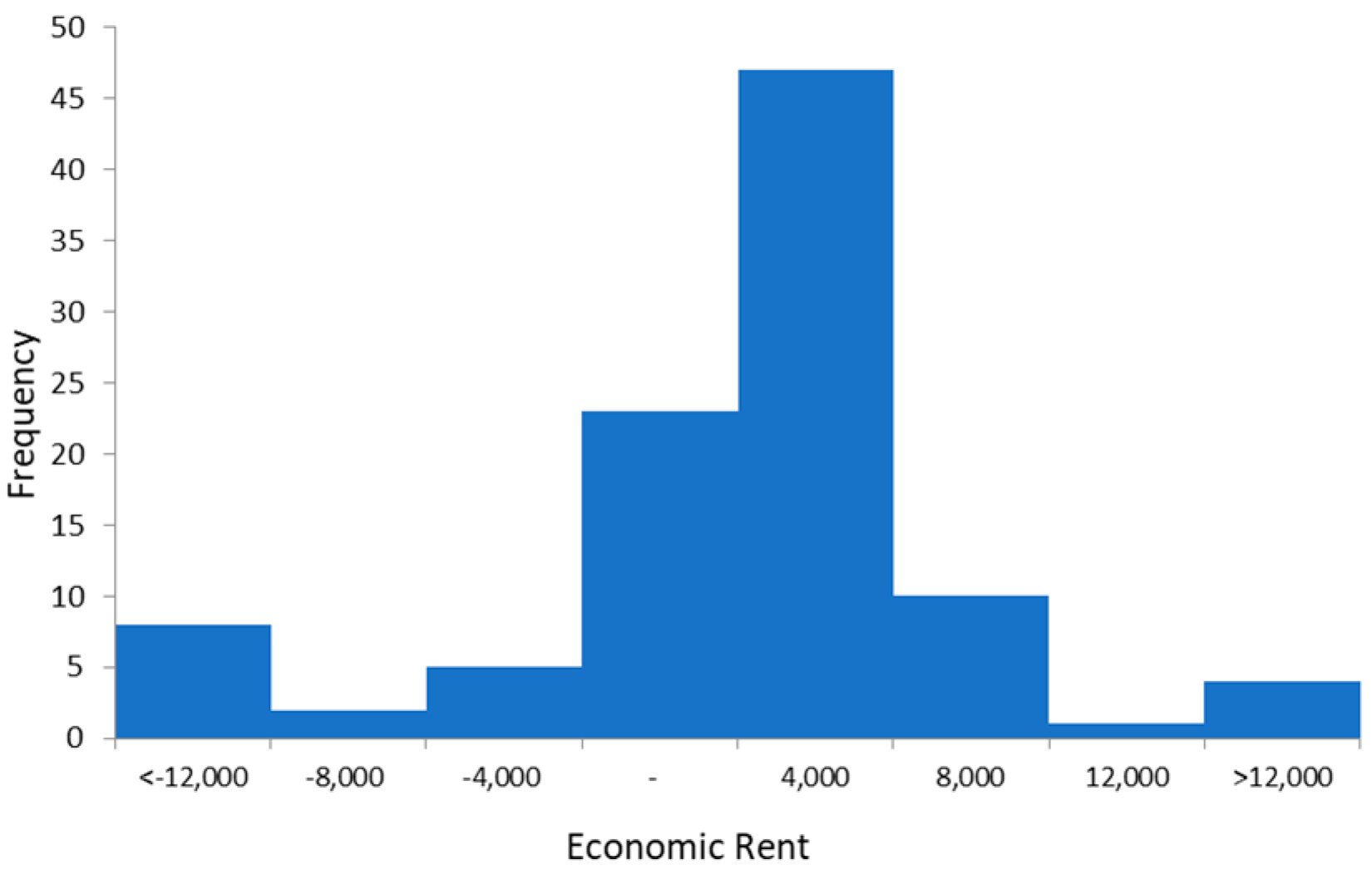
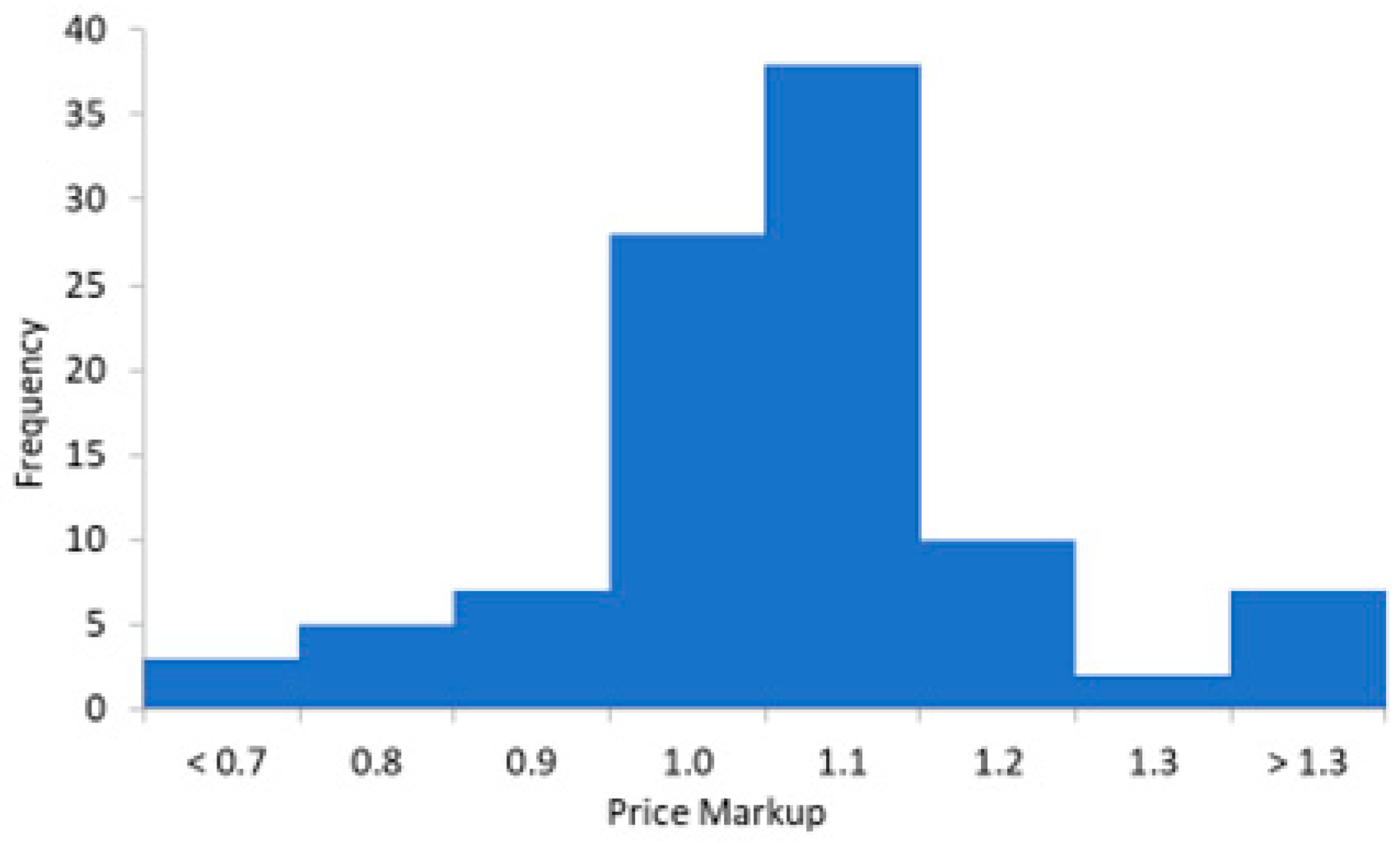
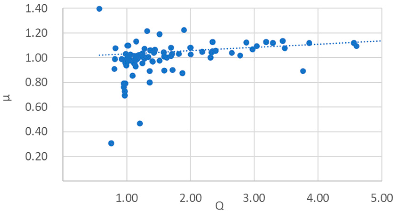
Across the years, market markup is consistent at unity and largely shows consistency at the industry and sector levels. Most firms earn some level of economic rent with a µ > 1 (Figure 1 and Figure 2). While the market Tobin’s Q is estimated as equivalent to the adjusted markup, firm values for Q are found to be generally higher than their corresponding µ (of which the medians are 1.36 and 1.02, respectively) whereby the distribution for Q is characterised by a number of liability-heavy balance sheet financial firms with Qs that are closer to unity and with a larger right tail (Figure 2, Figure 3, Figure 4, Figure 5 and Figure 6). This difference is also shown by the measure Q/µ (Table 1).
Seven firms meet the definition for significant markup with the industry/sector membership being limited to the real estate, technology/media and financial services/equity investment industries (Table 2).
5. Discussion
My approach avoids the need to estimate marginal costs, as required by other more recently developed methodologies. I use audited expenses to determine income, as well as labour, financing, depreciation, and other production input costs. In doing this, I assume no rent is paid to labour, and that any rent paid to other inputs should be recorded and attributed as rents earned by those suppliers. Using firm-specific Betas, I am able to construct the specific costs of equity for firms and apply them to the book value of equity in order to impute the total costs of equity and hence rents and so the price markup of firms. The integrity of firm financial balance sheets, income statements and in particular the total equity and income are therefore critical to the validity of outcomes for my method; these are discussed below.
5.1. Other Findings from the Literature
My estimations of the markup are lower than those of recent reports which ranged from 1.1 to 1.67 (Table 3). However, they may more closely match the results of those methodologies that determine profit share as a residual after calculating the capital and labour shares (Barkai 2020; Caballero et al. 2017; Gutiérrez 2017). The makeup of the FTSE 100 index, which is largely devoid of technology firms and is predominated by materials (mining), financials, consumer, energy, and industrials, should be considered when comparing with the results of other studies that are predominantly from the US. The UK’s ONS results (1.22–1.27) were based on the method of De Loecker and Warzynski (2009) and are notably lower than the US results when using the same approach (De Loecker and Warzynski 2009; De Loecker and Eeckhout 2018; De Loecker et al. 2020). Autor et al. (2020) demonstrated that the labour share in the UK was remarkably stable between 1970 and 2010, which is a phenomenon that stands in stark contrast to other OECD countries and suggests more moderate markup levels in the UK.
This study also found that of those firms earning an economic rent, five firms contributed an excess of 50% of the total rent earnt by the FTSE 100. This, coupled with the longer right-hand tail for markups (Figure 2) is a finding consistent with other studies (De Loecker et al. 2020; Traina 2018). These higher markup firms are characterised by the service and technology-orientated sectors, a phenomenon which has also been seen in the UK-specific ONS data. On the other side of performance, 43% of the firms in my analysis had a markup of less than one; Hall (2018) found that to be the case for 30% of firms.
5.2. Model Sensitivity
The return of the market (Rm) is not an independent variable in the model. The dynamics of the markup with respect to changes in the risk-free rate, Beta, total equity, and income are shown in Table 4. While an investor may assume differing risk-free rates, this has no, or limited, influence on model calibration given ∂µ/∂Rf > 0 if β > 1 and vice versa (19). In the case where either the Beta, revenue or total equity are underestimated, the price markup will be overestimated (∂µ/∂β, ∂µ/∂PY and ∂µ/∂T are all less than zero (20)–(22)). The opposite holds for income (23).
It further holds that changes in income have a more substantive impact on the level of price markup than changes to either total equity or revenue.
Proposition 4.
Proof of Proposition 4.
Equation (25) holds if PY3 > T2. Rm (simplifying for β = 1), which is highly likely given the magnitude of the cubed term (and is the case for all FTSE 100 firms for the period studied).
Equation (26) holds if (I/T)2 < Rm, which we would generally imagine to be the case. In this data set, the ratio of income to total equity (for the market) is close to one to ten (the square therefore being 1/100), with the return of the market also being at a similar level (9.76%).
Equation (27) holds if I2 > T which we would generally imagine to be the case and see as much in this data set. □
I model and demonstrate the effect of changes in these predicating variables as shown in Table 5.
5.3. Data Veracity
Given market Beta is defined by unity, as demonstrated in (24), income is the predicating variable with the greatest magnitude of effect within the model. Could income somehow not be accurate as stated in company reporting? In the case where the firm uses mechanisms such as transfer pricing to take advantage of corporate tax arbitrage in different jurisdictions a lower income will be reported and thus the price markup will be underestimated (23). On balance, it seems more likely that any transfer pricing involving UK legal entities would be to reduce income, given the existence of other lower tax jurisdictions. Liu et al. (2017) reported on this practice specific to the UK, i.e., that incomes may be under reported. Lower transfer prices would equally reduce revenue, which would at the same time decrease the markup. However, as we see in (24) and in Table 5, this has a non-material impact on the markup, i.e., the net effect of low transfer pricing will be to decrease the reported markup. In a similar fashion, intercompany liabilities (i.e., loans) of a multinational could be constructed to extract interest payments and thus reduce income.
The market valuation of assets and liabilities may differ to book values and so misrepresent true total equity. With most firms owning and not leasing their capital stock, accurate measurement may be frustrated. A prevailing view is that the capital stock and thus equity may be underestimated. Corrado et al. (2009) and Rivera-Padilla (2023) pointed to the growing economic importance of intangible assets including patents, copyrights, and brand value which have been historically excluded from balance sheet and public data sources; the same may be true for software and R&D (Barkai 2020; Berry et al. 2019). In these findings (Table 1), those industries with the highest Tobin’s Qs are those associated with the employment of these inputs, namely, the technology and healthcare industries. An underestimation of the capital stock will result in an underestimation of total equity and thus an overestimation of the markup (22).
The Bank of England rate as used for the risk-free rate in this study was fairly stable for the studied period, only starting to rise in 2023 (the UK financial year ends in March, with Q1 2023 being the last data point in this study). Nevertheless, it is possible that firms can carry book value liabilities that are at odds with a current market rate. Depreciation should also be considered: imprecision in reporting will impact both the stated income and the capital stock as reported in the balance sheet. UK companies are governed, of course, by Generally Accepted Accounting Practice (UK GAAP), and it would seem unlikely that these, the largest UK audited and publicly held firms were/are somehow systematically gaming depreciation charges in order to recognise financial profits either earlier or later. Miles (1987) reported rare cases of erroneous valuation. Finally, Beta may be subject to estimate error: the Betas I use are trailing and for a fixed five-year period and this will clearly have an impact at the level of the firm (24), but that is not the case for the market, given the market Beta will be equal to one. This leaves the possibility that a suppression in reported income would mean the markup is under-reported, while the quite likely possibility of underestimation in total equity will result in an over-reporting of the markup.
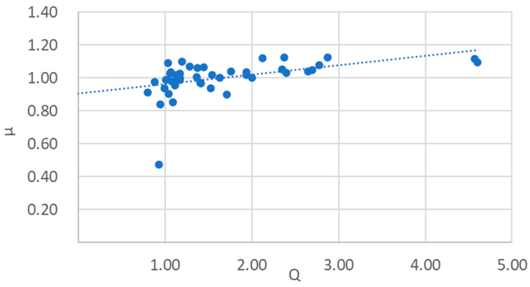
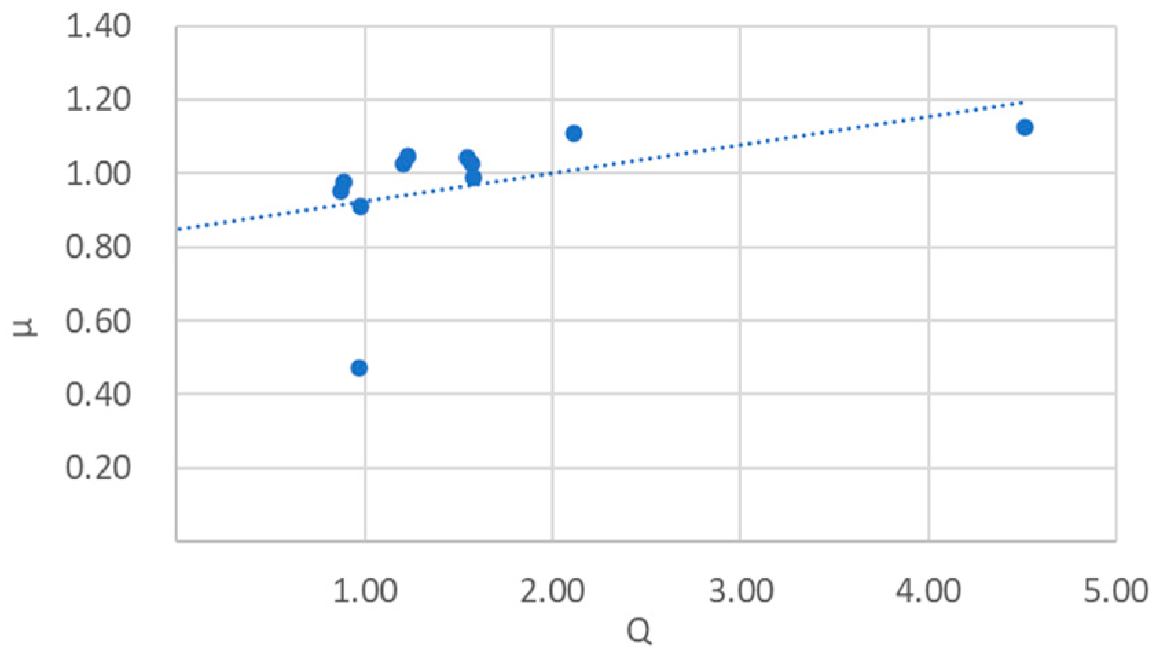
5.4. Regression Analysis
This study is, to my understanding, the first to propose and offer a proof that µ = Q. However, this empirical analysis suggests generally higher levels of Tobin’s Q than for the corresponding firm’s price markup: a regression analysis (Figure 4) gives a best fit10 of µ = 0.0261Q + 1.0041. A factored adjustment to the total equity of 2.76 achieves a least-squares fit for 2 and gives a market markup and Tobin’s Q of 0.86. Could the FTSE 100 price markup have been below one for the studied period and could the equity have been underestimated to this degree? With sunk costs and intangibles accruing no charges, we are reminded that it is perfectly possible for firms to turn profits whilst having a markup below one as this data set specifically shows at the firm level. A factor of 2.76 seems high, nevertheless, this does further point to the possibility of an underestimations of firms’ book value equities and provides this work with a lower bound result for the price markup of 0.86.
There are several other explanations for any empirical disconnect between the markup and Tobin’s Q that should be considered. Lower current price markups may be due to the firm investing in the erection of entry barriers to generate future higher markups; however, when considering the established nature of the FTSE 100 firms, as well as the industries in which they operate, this seems unlikely. Investment funds may be passive in nature or aimed with portfolio diversity in mind; furthermore, where they are through vehicles such as index trackers (i.e., of the FTSE 100) such unitary market-level investments would achieve a closer one-to-one equivalence between the price markup and Tobin’s Q (Table 1). It is of course possible that the economic outlook for many firms is simply better than was the case in near history, i.e., the expected markups are greater than the markups from the most recent past. Alternatively, in recognising that higher historic firm volatility with higher corresponding Betas will depress current markups, it might be that there exists a general optimism encompassing a less volatile future which would increase the markup. Finally, firms where the Q/µ is greater than unity might simply be overvalued.
µ = Q Implications
Tobin’s Q and the price-to-book ratio are long and well-established financial metrics and serve a purpose in investment decision making. My claim that the firm’s Tobin’s Q is equivalent to the price markup provides a mechanism through which to explain the firm’s Q in terms of expected marketplace pricing leverage and the ability to generate economic profits. This should therefore encourage future work in at least the fields of asset management, pricing, financial performance analysis and economics of the firm to explore this connection for insights and explanatory purposes.
From the perspective of the firm’s financial management, a Tobin’s Q of less than one may be seen as a product portfolio problem such that pricing elasticity does not allow for sufficient pricing levels to support an income that is at least equal to the costs of equity. The firm might better understand any abilities that they may have to increase pricing (although, surely, this must always be a present question for management), or the tasks of building brand equity and that of product-portfolio development and transition. For the firm with a Q in excess of one, the classical interpretation is that capital investment will be drawn in, thus restoring the Q to one. For this firm, the output level chosen may be in supporting an optimised price and for a premium product, i.e., there may be no interest in increasing volumes. The threat to this type of firm comes from external sources, i.e., where new entrants will desire a share of the rent. To maintain their position, management and owners are faced with decisions such as how to disburse profits, including the need to invest and innovate further to maintain their markup position. For the business-unit-based firm (irrespective of the overall level of Q), teasing out the Tobin’s Q for units may also be highly revealing.
5.5. Firms with Significant Markup
SGRO (markup 3.5) reported levels of income and economic rent that were greater than revenue: certain property gains were realised according to the UK’s IAS 40 accounting standard. Land is historically associated with economic rent, and the ONS data estimate real estate markup from 1.84 to 1.91 for the equivalent period, where as my measure delivered a result of 0.47. This likely demonstrates the need for analysis over extended time periods given the possibility of windfalls or accounting practices.
RMV (markup 2.3) and AUTO (1.9) both operate within the media sector of the technology industry, and they employ business models digitally connecting consumers with businesses, i.e., estate agents and car dealers, respectively. Consumers and businesses may aggregate towards single digital domains that benefit from network effects (Berry et al. 2019) which Autor et al. (2020) refer to as ‘superstar effects’ and which may explain the consistent higher level markups observed. The financial industry covers 10 different sectors with an overall markup that is less than unity. However, each of III (markup 1.8), HL (1.7), SMT (1.4) and PSH (1.4) are firms that may be characterised as investment entities (i.e., trusts/holdings/private equity/venture capital). Such markups may be interpreted as an alpha generated by the fund manager. Those parts of the alpha that can be attributed to rent might be subject to an appropriate taxation statute (Stiglitz 2015). These firms, according to the business models of the industrial sectors in which they sit, are likely to have particularly low if not zero level marginal costs (consider the marginal costs in adding a car to a website, or an additional set of funds to a portfolio), hence we can imagine pure economic rent earned from the marginal transaction.
The five banks all had negative rent and price markups that were less than one: performance was consistent over the period with limited variability. The healthcare industry (markup 1.11) and more specifically the pharmaceuticals and biotechnology sector rely on patent law to support R&D investment and their business models. To the extent that such assets are off-balance-sheet, price markups may be overestimated. Nevertheless, the markups as reported appear modest. Patent lengths could theoretically, be optimised to manage any emergence of longer-term rents. The historic association of utilities and energy with markups (Verbruggen 2022) are not borne out in this analysis (which had markups of 1.05 and 0.98, respectively). That consumer staples (1.04) have higher markups than consumer discretionary (0.99) may also be notable and a function of the elasticities for these respective sector groups.
5.6. Policy Implications
While taxation on labour, capital, or consumption may promote a government’s equity goals, basic economic theory shows that taxes have distortionary effects on volumes and thus reduce efficiency. In cases where economic rents are earned, taxation will not influence the firm’s production output behaviour; thus, rents are an attractive taxation target (Devereux 2019). This study finds that 2.6% of the revenue for all FTSE 100 companies is channelled to rent. However, practical vehicles that enable moves away from taxing corporations’ financial incomes to those of economic profit are wholly lacking in the literature, presumably for the good reason that such moves would present near insurmountable challenges. Whereas financial profits are easy to calculate, economic profits are not (as outlined in the above introductory discussion) and they would also require an entire shift in what are highly developed, ingrained systems and processes of taxation across firms, auditors, and government. There exist other hurdles that must also be managed. One must settle on a method for the computation of the price markup (even then, one can imagine the need for significant and ongoing arbitration). How would one handle those firms with a negative rent? The base (rent) of 2.6% for revenues is far short of the post-tax income base which represented 13.4% of revenues. In addition, this base also covers fewer firms, and so indicates any attempt to implement a taxation to rents would not be with an abandonment of the traditional tax to corporation income. Finally, in the absence of global agreements, first movers might also face particularly significant risks of capital flight.
The debate must also contemplate that not all rent can be deemed as bad. Innovations serve to destroy the old with the promise of productivity gains benefiting all of society (Schumpter 1942); Antonelli and Gehringer (2017) have more recently developed this orthodoxy. Clearly, the prospect of a 100% tax to rent removes all reward and incentive: the question then becomes how much rent might be allowed and how might the trade-off be determined (Boldrin and Levine 2008). Investment-derived innovations typically rely on intellectual property and thus rents can be (and are) modulated optimally according to patent terms (Gilbert and Shapiro 1990; Encaoua et al. 2006; Judd et al. 2012).
One exception where a tax to rent may present greater degrees of feasibility is land, given its inherent inelasticity11 (see Edenhofer et al. (2015) for an elaboration of the original work by Henry George). Schwerhoff et al. (2020) identified the introduction of a land tax as a type of part expropriation: the residual value of the land will fall by a factor related to the taxation rate, which they justify, given the control rights (i.e., how the land is to be used) remain with the owner and that any further investment by the landowner would be retained as a return to capital. These authors also point that the availability of more comprehensive land valuations opens the possibility for land taxes, which have otherwise hitherto not been typically employed by government. Any unfavourable change in the taxation statute will always be (financially) painful to the investor; however, in this sense, we might see the introduction of a land tax as no different in nature to an increase in, let us say, the corporate tax rate. Furthermore, under the assumption that a government seeks to maintain the tax take as neutral, other groups will benefit from the lowering of other taxes; thus, there will be an efficiency gain. We would also do well to remember that land is not mobile: owners cannot seek other lower tax jurisdictions.
Coupled with the post COVID-19 rebound, Russia’s invasion of Ukraine has caused a general inflationary pressure on energy prices and a corresponding rise in the profits for energy firms. This has reintroduced an active policy debate concerning windfall taxes (Fuest and Neumeier 2023; Baunsgaard and Vernon 2022). Again, the rationale for such taxes seems clear: these profits appear to be excess profits (rents). They also correspond directly to increases in household expenditure in terms of paying for increased energy bills (as well as other consumer products requiring energy as a factor of production). As such, the debate extends with an additional political significance. On this apparent basis of such obviousness, many economists support such windfall taxes. In the UK specifically, the Energy Profits Levy (EPL) (HM Revenue and Customs 2024) has been implemented with a taxation rate of 75% through to 2028.12 However, it is striking to note that from this data set and my definition for the price markup, the markups for the two FTSE 100 energy companies remain modest (Table 6). The UK government estimates that the measure will not have significant macroeconomic impact. However, while the empirical evidence for the effects of windfall taxes is limited, recent implementations have produced negative evaluations (Lazzari 1990, 2006; Rao 2018): production output, employment, and investor certainty may each be reduced. The perennial problem of agreeing the method for separating the windfall from the reward of higher risk investment remains (Antoniou et al. 2000), and any nominal rate will only be the same in real terms for unrealised profits if the mix between financial and economic profits remains the same, which seems unlikely: as such, the future real rate is therefore uncertain. Energy windfall taxes are further complicated given the current political agendas include the desire to secure greater degrees of energy self-sufficiency as well as the transition to renewables, both of which require investment and which critics of windfall taxes cite as being disincentivised in high tax and uncertain environments.
The notable results for RMV and AUTO, i.e., two of the three technology/media firms in the index, confirm the need for regulators to closely scrutinise consolidation in these categories. As with advertising on social media, the consumer is, in reality paying through a downstream purchase. Moreover, in the case of cars and houses, the payment is truly buried with the final product cost, which is likely to be high and financed through debt. These costs are not necessarily apparent to the user, and they are not directly related to the volume or timing of use. A doubling of price to the advertiser, which is then passed on to the end consumer, will remain small as a fraction of the acquisition cost of the car or house. Regulatory action must be measured with the knowledge of the undoubtable consumer benefit from the provision of product choice and one-stop shopping these services provide.
6. Conclusions
By employing a definition for price markups based on economic rent and firms’ costs of equity, I find moderate levels of price markup (0.86–1.07) for the UK’s largest firms, which are lower than those found in other recent reports, but the findings of this study are more congruent with the methodology of calculating profit share as the residual from labour and capital shares (Barkai 2020; Caballero et al. 2017; Gutiérrez 2017). Income, followed by total equity are the most sensitive variables in the model. While the result of µ = 0.86 (which is based on an underestimation of total equity) may be considered a lower bound, the multinationals’ financial management of income (i.e., reducing it) could see the markup exceeding my principal result (0.99). Nevertheless, a 50% underestimation of income only increases the markup to 1.07 (Table 5). My generally lower results do fit better with the previously described near past macroeconomic experience. Those firms who do enjoy significant price markups are limited by their industry and sector (real estate, technology/media and financial services and equity investment) (Table 2) as well as by aspects of their business models that may explain their ability to charge such rents.
I offer a formal proof that such expected markups are equal to Tobin’s Q (µe = Q) and show a near equivalence at the level of the market between the two ratios; however, they also see differences in the distributions for the set of FTSE 100 firms with generally higher results for Tobin’s Q. That the markup can be derived in such a relatively uncomplicated way through the computation of Q may give each of the firm’s managers, investors, and regulators an additional ratio with which to work. Researchers might utilize this finding to translate the results in certain fields (e.g., asset management) in terms of pricing and vice versa.
‘Permacrisis’ became the Collins Dictionary’s word of the year in 2022. Crises create instabilities and disruption which can be anticipated to lead to supply shortages and thus to price markups (at least in the short run). Defence firms may prosper in times of war, vaccine manufacturers during pandemics and energy companies in an environment of conflict, sanctions and cartel quotas. The current global situation therefore points to the need to better anticipate such firm windfalls and to ascertain as to whether they should be subject to extraordinary taxation (and if so how). If we agree rents can exist, a windfall is simply a periodic but non-persisting rent. It seems governments (and others) are identifying such windfalls as favourable reports of income, which depart from the firm’s historic norms and, not through any of the literature’s derived methods. The jury remains out with respect to the efficacy of windfall taxes (i.e., more empirical evidence is certainly needed), and it seems likely that particular and specific decisions will always be required according to the individual case, given the degrees of heterogeneity involved. Nevertheless, economic theory, as well as derivations of the markup and changes to the markup, should surely be called upon as any part of such assessments.
Whereas regulators in advanced economies have considerable experience in the oversight of natural monopolies, such as utility providers, the advent of newer service-based firms where network and platform effects may produce market power present areas where new expertise and understanding will be required: the ultimate tools for the regulator remain the breaking up of the firm or the blocking of mergers and acquisitions. Of note, most recently (2022–2023), and contrary to other sovereign regulators, the UK’s Competition and Markets Authority (2022), citing a lessening of competition, higher prices, fewer choices and less innovation, achieved concessions from Microsoft before approving their acquisition of Activision Blizzard.13 The recent efforts to develop measures of the markup should be applied to build better confidence in the estimation of land markups, as well as to examine their persistency. This may yet persuade and support government treasuries to implement some form of land tax.
Caution should be taken given the limited company membership (FTSE 100) and the relatively short period I have studied. This method relies on the accuracy of firm’ income and balance sheet statements, whereby income and total equity are demonstrated as variables of significant dependence, that come with the potential for misreporting. This work cannot account for a firm’s payment of other rents, such as, for example political or to labour. Nevertheless, this method should be generalisable to all firms and available data sets. Indeed, future research might expand this method to wider market data and to that of the US, where most research has historically been conducted, to better compare results. An application of the methodology to a wider time period might also assist the debate with respect to the relationship between markups and the business cycle. This work should also encourage the further characterisation of any differences observed between µ and Q. More generally, the further development of methodologies to accurately measure price markups are crucial for both economists and policy makers in understanding inequalities, market power, the results of mergers and acquisitions, and international trading arrangements.
Funding
This research received no external funding.
Data Availability Statement
Data available upon request.
Conflicts of Interest
The author declares no conflict of interest.
| 1 | This may be explained by manufacturing level non-neutral technological differences. |
| 2 | The Lerner Index ([P-MC]/P). Notably they found no relationship between Tobin’s Q and concentration. |
| 3 | The profit (π) will be this sales price minus the cost (T0 + L): π = ENt + T0 + L − T0 + L = ENt. |
| 4 | United Kingdom Debt Management Office. Available online: https://www.dmo.gov.uk/data/ExportReport?reportCode=D4H (accessed on 6 October 2023). |
| 5 | Office for National Statistics. Available online: https://www.ons.gov.uk/economy/inflationandpriceindices/timeseries/l55o/mm23 (accessed on 9 February 2023). |
| 6 | Sectors with three or more members only are highlighted. |
| 7 | Office for National Statistics (UK), using the methodology of De Loecker and Warzynski (2009). Available online: https://www.ons.gov.uk/economy/economicoutputandproductivity/productivitymeasures/articles/estimatesofmarkupsmarketpowerandbusinessdynamismfromtheannualbusinesssurveygreatbritain/1997to2019 (accessed on 20 December 2023). |
| 8 | Based on the expanded identity for price markup µ = PY/(PY − I + TRf + TβRm − TβRf). |
| 9 | Result from this study. |
| 10 | The outliers SGRO, RMV and AUTO are removed. |
| 11 | Hence Mark Twain’s quip ‘Buy land, they’re not making it anymore’. |
| 12 | An Energy Investment Security Mechanism (ESIM) has been put in place: The EPL will end if the 6-month average price for both oil and gas is at or below threshold prices ($71.40 dollars per barrel for oil and £0.54 per therm for gas). |
| 13 | A video gaming company. |
References
- Antonelli, Cristiano, and Agnieszka Gehringer. 2017. Technological change, rent and income inequalities: A Schumpeterian approach. Technological Forecasting and Social Change 115: 85–98. [Google Scholar] [CrossRef]
- Antoniou, Antonios, David G. Barr, and Richard Priestley. 2000. Abnormal Stock Returns and Public Policy: The Case of the UK Privatised Electricity and Water Utilities. International Journal of Finance & Economics 5: 93–106. [Google Scholar]
- Autor, David, David Dorn, Lawrence F. Katz, Christina Patterson, and John Van Reenen. 2020. The Fall of the Labor Share and the Rise of Superstar Firms. The Quarterly Journal of Economics 135: 645–709. [Google Scholar] [CrossRef]
- Bain, Joe S. 1951. Relation of profit rate to industry concentration: American manufacturing, 1936–1940. Quarterly Journal of Economics 65: 293–324. [Google Scholar] [CrossRef]
- Barkai, Simcha. 2020. Declining Labor and Capital Shares. The Journal of Finance 75: 2421–63. [Google Scholar] [CrossRef]
- Basu, Susanto. 2019. Are Price-Cost Markups Rising in the United States? A Discussion of the Evidence. Journal of Economic Perspectives 33: 3–22. [Google Scholar] [CrossRef]
- Baunsgaard, Thomas, and Nate Vernon. 2022. Taxing Windfall Profits in the Energy Sector. IMF Note 2022/00. Washington, DC: International Monetary Fund. Available online: https://www.imf.org/en/Publications/IMF-Notes/Issues/2022/08/30/Taxing-Windfall-Profits-in-the-Energy-Sector-522617 (accessed on 8 March 2024).
- Berry, Steven, Martin Gaynor, and Fiona Scott Morton. 2019. Do Increasing Markups berryMatter? Lessons from Empirical Industrial Organization. Journal of Economic Perspectives 33: 44–68. [Google Scholar] [CrossRef]
- Boldrin, Michele, and David K. Levine. 2008. Perfectly competitive innovation. Journal of Monetary Economics 55: 435–53. [Google Scholar] [CrossRef]
- Bresnahan, Timothy F. 1989. Empirical Studies of Industries with Market Power. In Handbook of Industrial Organization. Amsterdam: Elsevier, vol. 2, chap. 17. pp. 1011–57. [Google Scholar]
- Caballero, Ricardo J., Emmanuel Farhi, and Pierre-Olivier Gourinchas. 2017. Rents, Technical Change, and Risk Premia Accounting for Secular Trends in Interest Rates, Returns on Capital, Earning Yields, and Factor Shares. American Economic Review 107: 614–20. [Google Scholar] [CrossRef]
- Competition and Markets Authority. 2022. Microsoft/Activision Blizzard Merger Inquiry. Available online: https://www.gov.uk/cma-cases/microsoft-slash-activision-blizzard-merger-inquiry (accessed on 7 March 2024).
- Corrado, Carol, Charles Hulten, and Daniel Sichel. 2009. Intangible Capital and U.S. Economic Growth. The Review of Income and Wealth 55: 661–85. [Google Scholar] [CrossRef]
- De Loecker, Jan, and Frederic Warzynski. 2009. Markups and Firm-Level Export Status. NBER Working Paper Series 15198. Available online: http://www.nber.org/papers/w15198 (accessed on 15 December 2023).
- De Loecker, Jan, and Jan Eeckhout. 2018. Global Market Power. National Bureau of Economic Research, Working Paper 24768. Available online: http://www.nber.org/papers/w24768 (accessed on 10 February 2024).
- De Loecker, Jan, Jan Eeckhout, and Gabriel Unger. 2020. The Rise of Market Power and the Macroeconomic Implications. The Quarterly Journal of Economics 135: 561–644. [Google Scholar] [CrossRef]
- Devereux, Michael. 2019. How Should Business Profit Be Taxed? Some Thoughts on Conceptual Developments During the Lifetime of the IFS. Fiscal Studies 40: 591–619. [Google Scholar] [CrossRef]
- Edenhofer, Ottmar, Linus Mattauch, and Jan Siegmeier. 2015. Hypergeorgism: When Rent Taxation Is Socially optimal. FinanzArchiv/Public Finance Analysis 71: 474–505. [Google Scholar] [CrossRef]
- Eggertsson, Gauti B., Jacob A. Robbins, and Ella Getz Wold. 2021. Kaldor and Piketty’s facts: The rise of monopoly power in the United States. Journal of Monetary Economics 124: S19–S38. [Google Scholar] [CrossRef]
- Elsby, Michael W. L, Bart Hobijn, and Ayşegül Şahin. 2013. The Decline of the U.S. Labor Share. Brookings Papers on Economic Activity 2013: 1–52. [Google Scholar] [CrossRef]
- Encaoua, David, Dominique Guellec, and Catalina Martínez. 2006. Patent systems for encouraging innovation: Lessons from economic analysis. Research Policy 35: 1423–40. [Google Scholar] [CrossRef]
- Fuest, Clemens, and Florian Neumeier. 2023. Corporate Taxation. Annual Review of Economics 15: 425–45. [Google Scholar] [CrossRef]
- Gilbert, Richard, and Carl Shapiro. 1990. Optimal Patent Length and Breadth. The RAND Journal of Economics 21: 106–12. [Google Scholar] [CrossRef]
- Gutiérrez, German. 2017. Investigating Global Labor and Profit Shares. SSRN. Available online: https://ssrn.com/abstract=3040853 (accessed on 11 December 2023). [CrossRef]
- Hall, Robert. 1988. The Relation between Price and Marginal Cost in U.S. Industry. Journal of Political Economy 96: 921–47. [Google Scholar] [CrossRef]
- Hall, Robert. 2018. New Evidence on the Markup of Prices over Marginal Costs and the Role of Mega-Firms in the Us Economy. NBER Working Paper Series, Working Paper 24574. Available online: http://www.nber.org/papers/w24574 (accessed on 11 December 2023).
- HM Revenue and Customs. 2024. Energy Profits Levy: Energy Security Investment Mechanism. Policy Paper. Available online: https://www.gov.uk/government/publications/energy-profits-levy-energy-security-investment-mechanism-legislation/energy-profits-levy-energy-security-investment-mechanism (accessed on 7 March 2024).
- Judd, By Kenneth L., Karl Schmedders, and Şevin Yeltekin. 2012. Optimal Rules for Patent Races. International Economic Review 53: 23–52. [Google Scholar] [CrossRef]
- Karabarbounis, Loukas, and Brent Neiman. 2014. The Global Decline of the Labor Share. The Quarterly Journal of Economics 129: 61–103. [Google Scholar] [CrossRef]
- Lazzari, Salvatore. 1990. The Windfall Profit Tax on Crude Oil: Overview of the Issues. Congressional Research Service, Library of Congress. Available online: https://files.taxfoundation.org/legacy/docs/110805crs_windfall.pdf (accessed on 8 March 2024).
- Lazzari, Salvatore. 2006. The Crude Oil Windfall Profit Tax of the 1980s: Implications for Current Energy Policy. Congressional Research Service. Available online: https://liheapch.acf.hhs.gov/pubs/oilwindfall.pdf (accessed on 8 March 2023).
- Lindenberg, Eric B., and Stephen A. Ross. 1981. Tobin’s q ratio and industrial organization. Journal of Business 54: 1–32. [Google Scholar] [CrossRef]
- Liu, Li, Tim Schmidt-Eisenlohr, and Dongxian Guo. 2017. International Transfer Pricing and Tax Avoidance: Evidence from Linked Trade-Tax Statistics in the UK. Paper presented at Annual Conference on Taxation and Minutes of the Annual Meeting of the National Tax Association 110, Philadelphia, PA, USA, November 9–11; pp. 1–vii. Available online: https://www.jstor.org/stable/26794398 (accessed on 12 December 2023).
- Miles, John. 1987. Depreciation and Valuation Accuracy. Journal of Valuation 5: 125–37. [Google Scholar] [CrossRef]
- Piketty, Thomas. 2014. Capital in the Twenty-First Century. Cambridge, MA: Harvard University Press. [Google Scholar]
- Rao, Nirupama L. 2018. Taxes and US oil production: Evidence from California and the windfall profit tax. American Economic Journal: Economic Policy 10: 268–301. [Google Scholar] [CrossRef]
- Raval, Devesh. 2023. Testing the Production Approach to Markup Estimation. The Review of Economic Studies 90: 2592–611. [Google Scholar] [CrossRef]
- Rivera-Padilla, Alberto. 2023. Market power, output, and productivity. Economics Letters 232: 111318. [Google Scholar] [CrossRef]
- Schumpter, Joseph. 1942. Capitalism, Socialism and Democracy. New York: Harper & Brothers. [Google Scholar]
- Schwerhoff, Gregor, Ottmar Edenhofer, and Marc Fleurbaey. 2020. Taxation of Economic Rents. Journal of Economic Surveys 34: 398–423. [Google Scholar] [CrossRef]
- Sharpe, William F. 1964. Capital Asset Prices: A Theory of Market Equilibrium under Conditions of Risk. The Journal of Finance 19: 425–42. [Google Scholar] [CrossRef]
- Stiglitz, Joseph E. 2015. The Origins of Inequality, and Policies to Contain It. National Tax Journal 68: 425–48. [Google Scholar] [CrossRef]
- Syverson, Chad. 2019. Macroeconomics and Market Power: Context, Implications, and Open Questions. Journal of Economic Perspectives 33: 23–43. [Google Scholar] [CrossRef]
- Traina, James. 2018. Is Aggregate Market Power Increasing? Production Trends Using Financial Statements. SSRN. Available online: https://ssrn.com/abstract=3120849 (accessed on 11 December 2023). [CrossRef]
- Varian, Hal. 1987. Intermediate Microeconomics: A Modern Approach. New York: Norton, p. 396. [Google Scholar]
- Verbruggen, Aviel. 2022. The geopolitics of trillion US$ oil & gas rents. International Journal of Sustainable Energy Planning and Management 36: 3–10. [Google Scholar] [CrossRef]
Figure 1.
Economic rent (6 year total) distribution FTSE 100 firms (millions).

Figure 2.
Price markup distribution FTSE 100 firms.

Figure 3.
Tobin’s Q distribution FTSE 100 firms.

Figure 4.
Tobin’s Q and markup by FTSE firm.

Figure 5.
Tobin’s Q and markup by FTSE sector.

Figure 6.
Tobin’s Q & markup by FTSE industry.


Table 1.
Markup and Tobin’s Q by industry (bold), sector and year.
| 2018 | 2019 | 2020 | 2021 | 2022 | 2023 | Total—All Years | |||||
|---|---|---|---|---|---|---|---|---|---|---|---|
| Industry/Sector6 (No. of Firms) | µ | µ | µa | Q | Q/µ | σ (µ) | |||||
| Technology (7) | 1.19 | 1.15 | 1.14 | 1.13 | 1.12 | 1.07 | 1.13 | 2.52 | 4.51 | 3.99 | 0.04 |
| Media (3) | 1.29 | 1.25 | 1.26 | 1.22 | 1.24 | 1.21 | 1.24 | 0.95 | 1.17 | 0.94 | 0.03 |
| Health Care (6) | 1.08 | 1.10 | 1.08 | 1.16 | 1.03 | 1.22 | 1.11 | 2.02 | 4.11 | 3.71 | 0.06 |
| Pharmaceuticals and biotechnology (3) | 1.08 | 1.11 | 1.08 | 1.17 | 1.03 | 1.25 | 1.12 | 2.22 | 1.93 | 1.73 | 0.07 |
| Utilities (5) | 1.05 | 1.03 | 0.98 | 1.10 | 1.08 | 1.06 | 1.05 | 1.19 | 1.23 | 1.17 | 0.04 |
| Gas, water and multi-utilities (3) | 1.18 | 1.06 | 1.04 | 1.10 | 1.02 | 1.29 | 1.11 | 1.39 | 1.20 | 1.08 | 0.09 |
| Consumer Staples (10) | 1.07 | 1.05 | 1.02 | 1.08 | 1.03 | 1.03 | 1.04 | 1.07 | 1.33 | 1.28 | 0.02 |
| Industrials (10) | 1.08 | 1.00 | 1.02 | 1.00 | 1.04 | 1.03 | 1.03 | 1.24 | 1.54 | 1.49 | 0.03 |
| Support services (4) | 1.1 | 1.03 | 1.06 | 1.06 | 1.04 | 1.03 | 1.05 | 1.42 | 2.22 | 2.11 | 0.02 |
| Basic Materials (12) | 1.01 | 1.02 | 1.01 | 1.02 | 1.05 | 1.04 | 1.02 | 1.09 | 1.21 | 1.19 | 0.02 |
| Mining (6) | 1.00 | 1.02 | 1.00 | 1.02 | 1.06 | 1.04 | 1.03 | 1.09 | 1.17 | 1.14 | 0.02 |
| Consumer Discretionary (18) | 1.03 | 1.04 | 1.01 | 0.89 | 0.96 | 0.99 | 0.99 | 1.07 | 1.54 | 1.56 | 0.05 |
| Household goods and home vonstruction (4) | 1.03 | 1.03 | 1.06 | 1.04 | 0.96 | 0.94 | 1.00 | 0.98 | 1.11 | 1.11 | 0.04 |
| Media (3) | 1.01 | 0.95 | 0.98 | 0.79 | 0.94 | 1.02 | 0.95 | 0.95 | 1.17 | 1.23 | 0.08 |
| Travel and leisure (4) | 1.03 | 1.02 | 1.00 | 0.70 | 0.85 | 0.96 | 0.94 | 1.11 | 1.53 | 1.63 | 0.12 |
| Energy (3) | 0.97 | 1.00 | 0.99 | 0.85 | 0.99 | 1.01 | 0.98 | 1.02 | 0.89 | 0.91 | 0.05 |
| Telecommunications (3) | 0.95 | 0.85 | 0.94 | 0.98 | 0.94 | 1.07 | 0.95 | 0.90 | 0.88 | 0.92 | 0.07 |
| Financials (23) | 0.92 | 0.84 | 0.96 | 1.04 | 0.90 | 0.02 | 0.91 | 0.96 | 0.98 | 1.07 | 0.35 |
| Financial services (9) | 1.01 | 1.05 | 1.05 | 1.34 | 1.16 | 0.78 | 1.09 | 2.26 | 1.03 | 0.95 | 0.17 |
| Life insurance (3) | 1.00 | 1.01 | 1.00 | 1.04 | 0.94 | 1.05 | 0.99 | 0.99 | 1.01 | 1.02 | 0.04 |
| Banks (5) | 0.8 | 0.80 | 0.86 | 0.95 | 0.83 | 0.83 | 0.84 | 0.86 | 0.95 | 1.13 | 0.05 |
| Real Estate (3) | 0.47 | 0.49 | 0.40 | 0.50 | −3.19 | 0.25 | 0.47 | 0.71 | 0.97 | 2.07 | 1.35 |
| FTSE 100 | 0.99 | 0.99 | 0.99 | 1.00 | 1.00 | 1.00 | 0.99 | 1.07 | 1.06 | 1.07 | 0.01 |
Table 2.
Firms with significant markup.
| Company | Industry | Sector | µ |
|---|---|---|---|
| Segro PLC—SGRO | Real Estate | Real Estate Investment Trusts | 3.5 |
| Rightmove PLC—RMV | Technology | Media | 2.3 |
| Auto Trader Group PLC—AUTO | Technology | Media | 1.9 |
| 3I Group PLC—III | Financials | Financial Services | 1.8 |
| Hargreaves Lansdown PLC—HL | Financials | Financial Services | 1.7 |
| Scottish Mortgage Investment Trust PLC—SMT | Financials | Equity Investment Instruments | 1.4 |
| Pershing Square Holdings LTD—PSH | Financials | Financial Services | 1.4 |
Table 3.
Findings from the literature.
| Author | Year | Country | µ |
|---|---|---|---|
| De Loecker and Warzynski (2009) | 1994–2000 | Slovenia | 1.17–1.28 |
| Caballero et al. (2017) | 2008–2015 | US | 1.02–1.12 |
| De Loecker and Eeckhout (2018) | 1980–2016 | Global | 1.15–1.60 |
| De Loecker et al. (2020) | 1980–2016 | US | 1.21–1.61 |
| Barkai (2020) | 1984–2014 | US | 1.02–1.19 |
| Gutiérrez (2017) | 2014 | US | 1.21 |
| Traina (2018) | 2016 | US | 1.15 |
| Eggertsson et al. (2021) | 2018 | US | 1.22 |
| Hall (2018) | 2018 | US | 1.27 |
| ONS7 | 2018 | UK | 1.22 |
| ONS | 2021 | UK | 1.27 |
Table 4.
Derivatives.8
Table 4.
Derivatives.8
| (19) | |
| (20) | |
| (21) | |
| (22) | |
| (23) |
Table 5.
Effects of changes in predicating variables.
| Risk-free rate (Rf) | Rf | Rf | Rf = 1.92%9 | Rf | Rf |
| µ | 0.99 | 0.99 | 0.99 | 0.99 | 1.00 |
| Revenue (index) | PY | PY | 1.0 | PY | PY |
| µ | 0.99 | 0.99 | 0.99 | 0.99 | 0.99 |
| Beta | β = 0.70 | β = 0.85 | β = 1.0 | β = 1.15 | β = 1.3 |
| µ | 1.01 | 1.00 | 0.99 | 0.98 | 0.97 |
| Total equity (index) | 0.25 | 0.5 | 1.0 | 2 | 4 |
| µ | 1.06 | 1.04 | 0.99 | 0.91 | 0.79 |
| Income (index) | 0.25 | 0.5 | 1 | 2 | 4 |
| µ | 0.94 | 0.95 | 0.99 | 1.07 | 1.29 |
Table 6.
Markup energy/oil and gas producers.
| 2018 | 2019 | 2020 | 2021 | 2022 | 2023 | |
|---|---|---|---|---|---|---|
| BP PLC—BP | 0.97 | 0.99 | 0.97 | 0.81 | 0.99 | 0.96 |
| Shell PLC—SHEL | 0.97 | 1.00 | 1.00 | 0.86 | 0.99 | 1.05 |
Disclaimer/Publisher’s Note: The statements, opinions and data contained in all publications are solely those of the individual author(s) and contributor(s) and not of MDPI and/or the editor(s). MDPI and/or the editor(s) disclaim responsibility for any injury to people or property resulting from any ideas, methods, instructions or products referred to in the content. |
© 2024 by the author. Licensee MDPI, Basel, Switzerland. This article is an open access article distributed under the terms and conditions of the Creative Commons Attribution (CC BY) license (https://creativecommons.org/licenses/by/4.0/).
Share and Cite
MDPI and ACS Style
Hackworth, P. The Current and Expected Pricing Markup as Derived from the Capital Asset Pricing Model and Tobin’s Q and Applied to the UK’s FTSE 100. J. Risk Financial Manag. 2024, 17, 127. https://doi.org/10.3390/jrfm17030127
AMA Style
Hackworth P. The Current and Expected Pricing Markup as Derived from the Capital Asset Pricing Model and Tobin’s Q and Applied to the UK’s FTSE 100. Journal of Risk and Financial Management. 2024; 17(3):127. https://doi.org/10.3390/jrfm17030127
Chicago/Turabian StyleHackworth, Paul. 2024. "The Current and Expected Pricing Markup as Derived from the Capital Asset Pricing Model and Tobin’s Q and Applied to the UK’s FTSE 100" Journal of Risk and Financial Management 17, no. 3: 127. https://doi.org/10.3390/jrfm17030127