Enhancing pest control interventions by linking species distribution model prediction and population density assessment of pine wilt disease vectors in South Korea
 Inyoo Kim
 Youngwoo Nam
 Sinyoung Park
 Wonhee Cho
 Kwanghun Choi
 Dongwook W. Ko6*
- 1Department of Forest Resources, Kookmin University, Seoul, Republic of Korea
- 2Forest Entomology and Pathology Division, National Institute of Forest Science, Seoul, Republic of Korea
- 3Forest Ecology Division, National Institute of Forest Science, Seoul, Republic of Korea
- 4Industry Academic Cooperation Foundation, Kookmin University, Seoul, Republic of Korea
- 5Center for Environmental Data Strategy, Korea Environment Institute, Sejong, Republic of Korea
- 6Department of Forest, Environment, and Systems, Kookmin University, Seoul, Republic of Korea
Pine wilt disease caused by pinewood nematode is one of the most destructive forest diseases, and still spreading in South Korea despite the various control efforts. Japanese pine sawyer (JPS) and Sakhalin pine sawyer (SPS) are the main vectors of the disease. Understanding the distribution and density of the vectors is crucial since the control period is determined by the different emergence periods of the two vectors and the control method by its density and the expected damage severity. In this study, we predicted the distribution of JPS and SPS using Maxent and investigated the relationship between the resulting suitability value and the density. The population densities of JPS and SPS were obtained through a national survey using pheromone traps between 2020-2022. We converted the density data into presence/absence points to externally validate each species distribution model, then we used quantile regression to check the correlation between the suitability and population density, and finally we used three widely used thresholds to convert the model results into binary maps, and tested if they could distinguish the density by comparing the Rb value of biserial correlation. The quantile regression revealed a positive relationship between the habitat suitability and population density sampled in the field. Moreover, the binary map with threshold criteria that maximizes the sum of the sensitivity and specificity had the best density discrimination capacity with the highest Rb. A quantitative relationship between suitability and vector density measured in the field from our study provides reliability to species distribution model as practical tools for forest pest management.
1 Introduction
Pine wilt disease (PWD) has devastated the forests of East Asia and Europe (Zhao et al., 2008; CABI, 2021). The disease is caused by pinewood nematode (Bursaphelenchus xylophilus (Seiner et Buhrer) Nickle (Nematoda, Aphelenchoididae)), which quickly kills host pine species, hindering forest growth and causing economic and ecologic impacts (Shin, 2008; Mota et al., 2009; Futai, 2013). Pine sawyers are the main vectors of the pinewood nematodes which cause PWD (Kishi, 1995). Pine sawyers can form a symbiotic relationship with the pinewood nematode; pine sawyers disperse the nematode, and the nematodes inhabit the phloem tissues of the host trees eventually causing death, which can be used for oviposition by pine sawyers (Mamiya and Enda, 1972).
The forest in South Korea has been heavily damaged by the disease since its first introduction at Busan in 1988 (Yi et al., 1989). In the 2000´s PWD spread about half of the country through Jeollanam-do, Gwangwon-do, and Jeju-do province. By the end of 2010, PWD had spread through the entire country (Choi and Park, 2012). Due to its cultural and historical values, the host Japanese red pine (Pinus densiflora Siebold & Zucc, (Pinales, Pinaceae)), the most abundant tree species in South Korea, demands urgent PWD control (National Geography Information Institute, 2020). In South Korea, Japanese pine sawyer (JPS) (Monochamus alternatus Hope, 1843 (Coleoptera, Cerambycidae)) and Sakhalin pine sawyer (SPS) (Monochamus saltuarius Gebler,1830 (Coleoptera, Cerambycidae)) are the main vectors of PWD (Shin, 2008). JPS is known to play a major role in PWD dispersal as they carry more pinewood nematodes (Mamiya, 1972) and have greater dispersal ability than SPS (Kwon et al., 2018). Preemptive control of JPS and SPS distribution is crucial for preventing the spread of PWD. PWD control in South Korea is scheduled and prioritized by the emergence period of the two vectors, since the best practice is to eliminate the infected host trees before the spread (Kwon et al., 2011). As the emergence periods of the two vectors are different, controlling efforts should be made in May for the SPS habitats and in mid-June for the JPS habitats (National Institute of Forest Science, 2016).
Identifying the distribution and density of forest pests is essential to schedule and prioritize the control (Barbosa et al., 2012). The species distribution model (SDM) has been widely used to predict species distribution by correlating the occurrence or absence of the species with environmental variables, primarily in geographic space. (Elith and Leathwick, 2009; Merow et al., 2014; Peterson et al., 2015). Habitat suitability is the primary outcome of SDM, which represents the suitable combination of the environmental variables, the probability of occurrence when presence/absence data is used to build the model, or the relative likelihood of occurrence when a background point is used. (Pearson, 2010; Guillera-Arroita et al., 2015). Estimated habitat suitability is used to map geographic range and area to surveil, or control in case of forest pests (Padalia et al., 2014).
Previous studies focused on the distribution of PWD itself only using the occurrence points of PWD (Matsuhashi et al., 2020; Wang et al., 2022). Yet, PWD occurs and spreads in a complex relationship between pathogen, host, and vector. Despite the importance of the biotic interactions highly dependent on the ecological traits of vectors, not many studies considered the biotic interaction between the pathogen, host, and vector in PWD SDM (Tang et al., 2021; Yoon et al., 2023), or predicted the distribution of each vector separately (Estay et al., 2014). In South Korea, Kwon et al. (2006) reported that the distributions of JPS and SPS were separated with a 13.2°C mean annual temperature threshold. JPS was distributed in the southern part of the country in warmer climate regions and SPS in the relatively cold northern regions. Kim et al. (2016) used the CLIMEX model to predict the distribution of JPS by using life cycle temperature requirements as the main variables.
The relationship between the distribution of the species and the density has been generalized that the population density is highest near the center of species distribution and declines towards the boundary, with the assumption that the spatial variation in density will depend on the combination of environmental variables interacting with the species` niche (Hutchinson, 1959; Brown, 1984). Despite the intuition that habitat suitability should explain the species’ density, several studies have tested the relationship between them and had opposite results, with some reporting the relationship generally none and statistically significant confounded only to some species (Pearce and Ferrier, 2001; Nielsen et al., 2005), while VanDerWal et al. (2009) found strong and consistent relationship in most of the 69 rain forest vertebrates in the Australian wet tropics. Nonetheless the debate, population density data is not often related to the SDM habitat suitability due to its expense and time-consuming effort (Tôrres et al., 2012). Nevertheless, the data is valuable, containing the presence/absence of the species and the degree of abundance in spatial variation, possessing the potential for further analysis.
In this study, we used a machine learning based SDM, Maxent (RRID:SCR_021830), to predict the distribution of two vectors of PWD in South Korea and explored the relationship between suitability and density. The density data of JPS and SPS was obtained through a nationwide survey between 2020-2022. First, we converted the density data into a presence/absence data format to validate the SDMs externally. Second, we used quantile regression to test the correlation between the suitability and the in-situ sampled vector density. Finally, we used three widely used thresholds to convert SDM results into binary maps and tested if they could distinguish the density by comparing the Rb value of biserial correlation. By showing the quantitative relationship between SDM and vector density measured in the field, the study may provide better use of SDM as a practical tool for forest pest management.
2 Materials and method
2.1 Study area
The study area is the forested land in South Korea (longitude 125° 25’ 30” - 30° 7’ 60” E and latitude 38° 50’ 30” - 33° 54’ 30’ N) (Figure 1A). The forest covers approximately 64% (6,294,334 ha) of the country, consisting of 38.8% conifer forest, 33.4% deciduous forest, and 27.8% mixed forest (Korea Forest Service, 2022). Mean annual temperature ranges from 1.8 to 15.2°C (Figure 1B). The country is wide in the North-South direction and topographically complex, with mountain ranges stretched along the East Coast, forming diverse regional climates (Park et al., 2009).
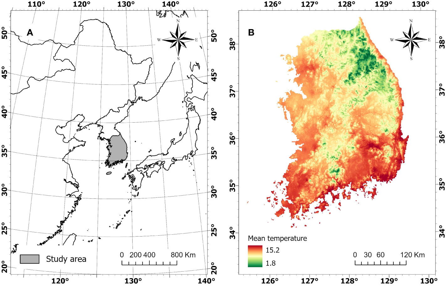
Figure 1 Geographic location of Korean Peninsula (A) and mean annual temperature of South Korea (B).
2.2 Occurrence data of vectors
Maxent uses presence locations as input, along with a set of environmental variables. The occurrence geographical coordinates of two vector species are compiled mainly from three sources; (1) the field survey provided by the National Institute of Forest Science, (2) a previous study on JPS and SPS distribution by Kwon et al. (2006), (3) the online database of Global Biodiversity Information Facility (GBIF) database (Kwon, 2022a; Kwon, 2022b). A total of 86 JPS and 112 SPS present points are collected. The occurrence data are commonly clustered and inherent with sampling bias. Such bias can increase the correlation in certain locations and overfit the model, so that we need a preprocessing of the data (Boria et al., 2014). We used spThin R package (ver. 0.2.0) to thin the occurrence location within 5km (Aiello-Lammens et al., 2015), which is known to be the maximum natural dispersal distance of JPS (Kwon et al., 2018). The final number of occurrence points used in the models is 78 for JPS and 87 for SPS (Figure 2A).
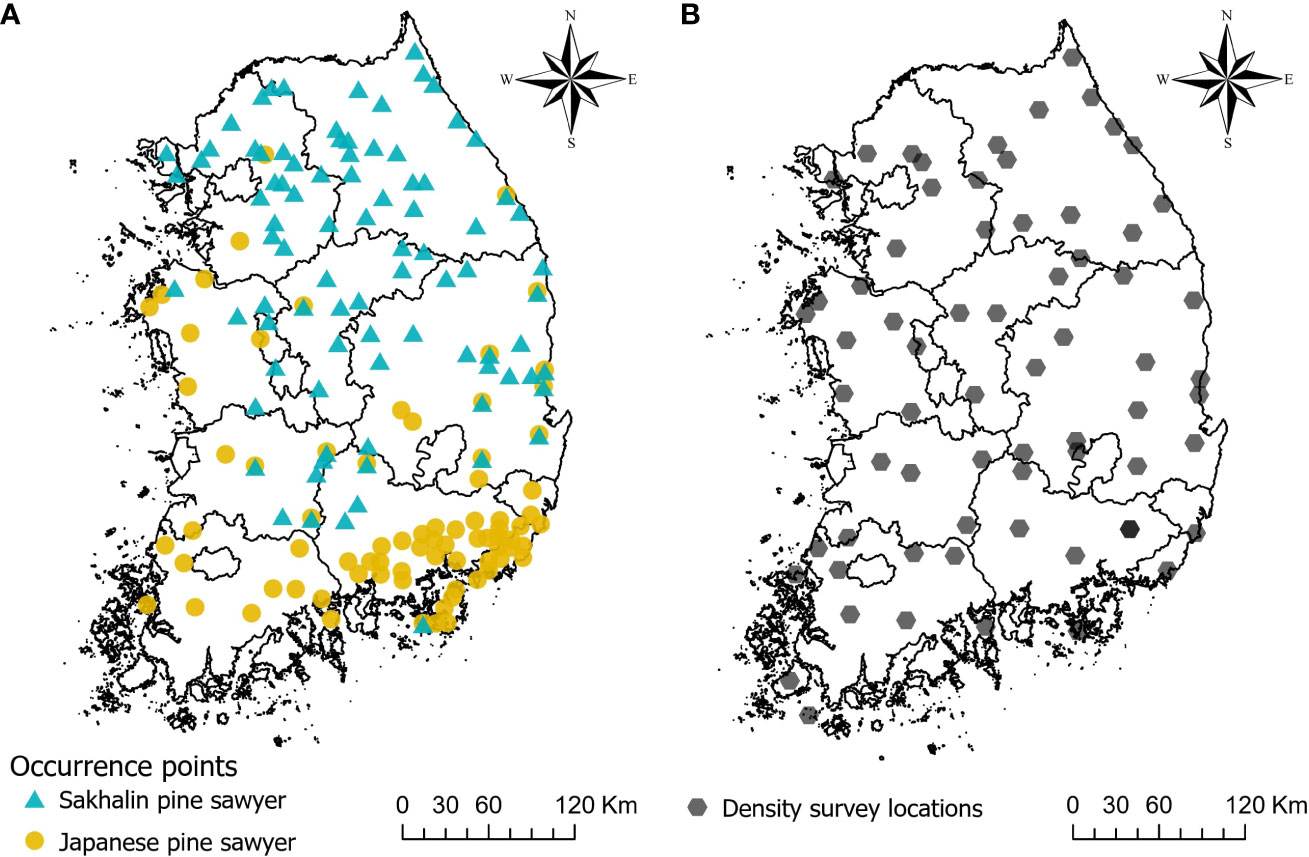
Figure 2 Map showing occurrence points of Sakhalin pine sawyer and Japanese pine sawyer used in the model (A), and density survey locations obtained by pheromone traps (B).
2.3 Environmental variables
We used the bioclimatic maps from worldclim (ver 1.4) with 1km resolution as predictive variables (Hijmans et al., 2005). Among 19 variables, bio8, bio9, bio18, bio19 are excluded due to the discontinuity problem (Booth, 2022). Next, SDMtune r package (ver. 1.1.6) is used to remove variables with high correlation with Pearson correlation coefficient over 0.7 for reducing the effect of multicollinearity among variables and increasing the interpretability of the model (Vignali et al., 2020). The remaining variables are again selected with permutation importance values over 15. The final variables used in models are the mean temperature of warmest quarter (bio10) and precipitation seasonality (bio15) for JPS and annual mean temperature (bio1) and temperature seasonality (bio4) for SPS.
2.4 Species distribution model and evaluation
Maxent (ver. 3.3.4) is used to predict the distribution of each vector (Phillips et al., 2017). The model predicts the potential distribution of the species that maximizes the entropy (Phillips et al., 2006). Maxent performs well with only the occurrence points and in small datasets (Pearson et al., 2007). The model is flexible and can fit various patterns including linear and non-linear relationships between explanatory and predictive variables (Elith et al., 2011). As the method is prone to overfitting when using the default settings, we used the ENMeval r package (ver. 2.0.3) for feature class selection and regularization multiplier settings to overcome the overfitting of the model (Muscarella et al., 2014). A combination of the two with the lowest 10% training omission rate is selected for each model. A model with a low omission rate is considered to have a high discrimination ability, and the model is not overfitted (Peterson et al., 2012).
The background points (or pseudo-absences) are the location data created by the user to contrast from the occurrence location. Background points are created using the “grid method” suggested by Elith et al. (2010). The idea is that background points should also have the geographic bias that occurrence points have in order to minimize their impact on the model. Gaussian kernel density of sampling localities tool from SDMtoolbox (ver. 2.0) is used to create the bias grid (Brown, 2014). And create spatially balanced point tool from ArcGIS pro (ver. 2.5) is used to create 10,000 points outside the 4km buffer from the occurrence points (Barbet-Massin et al., 2012; Esri Inc, 2020).
We divided the occurrence data into 75% of training data and 25% of cross-validation data by geographic division. The division is divided by longitude and latitude, each containing one-quarter of occurrence data. Fitting the model with spatially divided occurrence data reduces spatial autocorrelation (Radosavljevic and Anderson, 2014). Each model is repeated 500 times.
We converted the density data into presence/absence format for the external validation of the model, where survey location with 0 density as absence and presence if any single individual was found. Threshold independent area under the curve (AUC) is used to evaluate the models (Phillips and Dudík, 2008). AUC is the area under the receiver operating characteristic (ROC) curve. A high AUC value indicates high accuracy and good model performance (Franklin, 2010). The evaluate function in Dismo package (Ver.1.3-14, Hijmans et al., 2017) is used to calculate the validation AUC, as it is the same internal function used in ENMeval package to calculate the cross-validation AUC.
2.5 Monochamus spp. population density data
The density of JPS and SPS was surveyed in South Korea using a pheromone trap between 2020 and 2022 (Figure 2B). Each survey was performed in one site in every 40 km * 40 km grid that evenly divided the whole country, except for the islands and inaccessible areas such as military security zones. A total of 64 locations with JPS and SPS density information are obtained. The trap locations within the forest were determined based on where PWD host trees were abundant. Since the survey was done with the aid of the local governments with varied budget conditions, the number of traps varied by location with an average of 19. Each trap was placed at least 10 m away from other traps in the forest. Since monochamol (2-undecyloxy-1-ethanol) is known as an attractant for species belonging to the genus Monochamus (Lee et al., 2018), pheromone lures (monochamol, EtOH, a-pinene) were hung on each trap to attract the vectors and were replaced approximately every 2 weeks after the traps were installed. We also used a mixture of 70% EtOH and antifreeze in traps as preservatives to prevent the decay of caught insects. Sampling periods were from May to July. Samples were moved to the laboratory at the National Institute of Forest Science in Seoul, South Korea. Monochamus beetle species were isolated from other cerambycid beetles and stored in bottles with 70% EtOH until identification. A total of 2,503 JPS were caught in the trap with a wide variation between the sites from 0 to 1,721 individuals, and 2,040 SPS were caught ranging from 0 to 308. The density of each site was calculated dividing the captured individual by the number of traps, and we transformed the value logarithmically due to high variability.
2.6 Relationship between SDM suitability and density
The predicted suitability value of each model is extracted from each density survey points as shown in Figure 2B, to analyze the correlation between suitability and density. First, we used quantile regression to test the correlation between suitability and density as continuous variables. Secondly, we used three widely used thresholds to convert the suitability map into binary and tested if presence/absence from the binary map could distinguish the density value by comparing the Rb value of biserial correlation.
Quantile regression is a method used to estimate functional relations between variables with unequal variation, which is common in ecology (Koenker and Bassett, 1978; Cade and Noon, 2003). An ecosystem is complex with the interaction of heterogeneous variations and demands different analytical approaches to investigate the relationships between variables (Kareiva, 1990; Brown et al., 2002; Austin, 2007). Quantile regression can estimate functional relations between variables for all conditional quantiles of a probability distribution (Cade and Noon, 2003). Ordinary linear regression was not applicable because the data was not normally distributed. Instead, quantile regression was used to examine the relationship.
Insect populations can vary significantly in time and space (Geier, 1966), affected by many factors such as biotic interactions or density dependence (Juliano, 2007). Past studies used the usual regression method that focuses on the changes in the mean of the variables and found no success in discovering the relationship between habitat characteristics and species´ density (Dunham, 1996; Thomson et al., 1996). In comparison, quantile regression can provide more information clouded by missing variables and have successfully identified the relationship between habitat and species response (Cade et al., 1999; Dunham et al., 2002; Cade et al., 2005; Schröder et al., 2005), and between SDM-driven suitability and the density (Elmendorf and Moore, 2008; VanDerWal et al., 2009).
In this study, the quantile regression of the upper quantile from 60th to 90th with an interval of 10 is used. Past studies on the relationship between habitat suitability and density showed the wedge-shaped spread of points between them, meaning the presence of unmeasured factors limiting the potential abundance (Dunham et al., 2002; VanDerWal et al., 2009). The model in this study was built only with bioclimatic variables; we anticipated a similar pattern and used the upper quantile for the regression. The result of quantile regression is evaluated with pseudo r square (or coefficients of determination) and slope for each quantile (Koenker and MaChado, 1999).
Also, we tested the relationship between suitability and density further by analyzing the density value between the presence/absence area in a binary-converted suitability map. Although the conversion of the suitability map into discrete categories can degrade the information of the results (Guillera-Arroita et al., 2015), a binary map is widely used for practical applications and to interpret the outcome (Araújo et al., 2004; Jiménez-Valverde and Lobo, 2007). Moreover, various threshold criteria are used to assess the model performance by creating a confusion matrix (Liu et al., 2011). The choice of threshold criteria depends on the study’s objective, and selecting the optimal criteria is challenging (Loiselle et al., 2003; Liu et al., 2005). To test which threshold criteria can better distinguish the density of vectors, we used three widely used threshold criteria to convert JPS and SPS habitat suitability maps into binary and tested the difference in density values between the presence/absence areas using biserial correlation. The threshold criteria used are 1) Threshold that sensitivity (Se) equals specificity (Sp), Se=Sp in short, 2) Threshold that maximizes the sum of the sensitivity and specificity, max(Se+Sp) in short, 3) Threshold that maximizes the sum of positive predictive value (PPV) and negative predictive value (NPV), max(PPV+NPV) in short. Biserial correlation is used to test the relation between one variable in continuous and the other variable in dichotomous (Sheskin, 2011). The higher coefficient Rb value means the variables have a strong magnitude of the relationship.
3 Results
3.1 Distribution of Monochamus spp.
The predicted distribution of two vectors were opposite of each other with few overlapping areas (Figure 3). For JPS, Precipitation seasonality (bio15) was the most influential variable with a permutation importance value of 68.2, followed by mean temperature of warmest quarter (bio10) of 31.8. Predicted suitability decreased with bio15 and increased with bio10, resulting in the JPS distribution in the southern part of South Korea along the coastline (Figure 4).
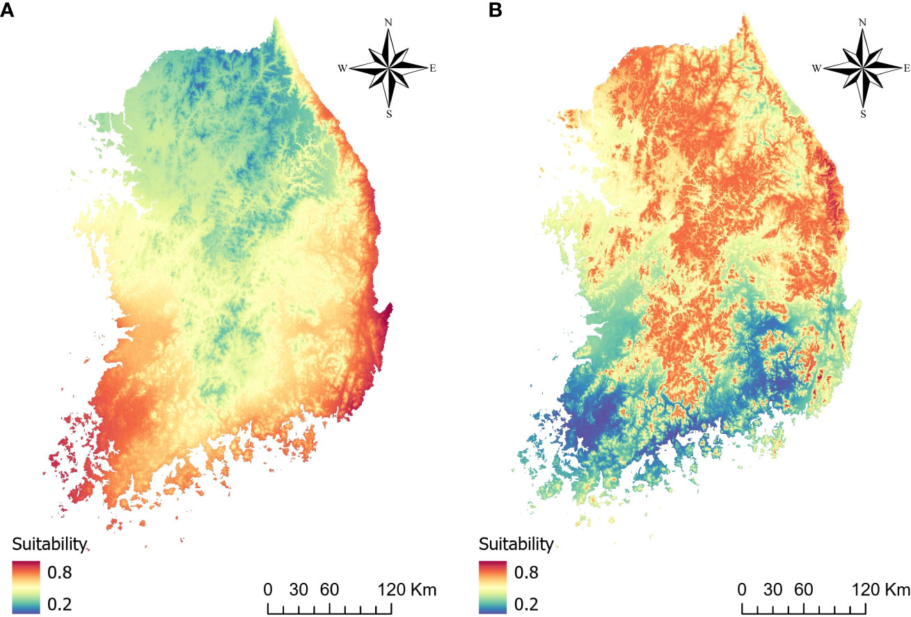
Figure 3 Predicted distribution of (A) Japanese pine sawyer and (B) Sakhalin pine sawyer.
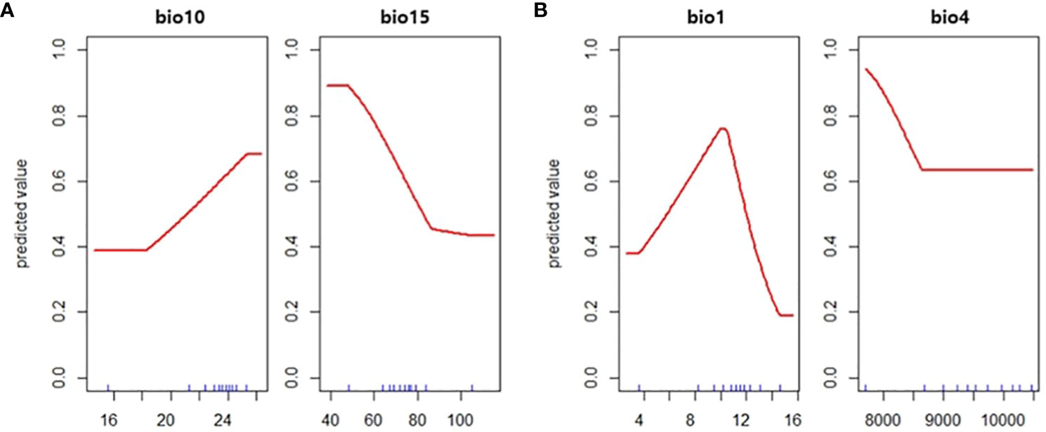
Figure 4 The response curve of the predicted value to (A) mean temperature of warmest quarter (bio10) and precipitation seasonality (bio15) in Japanese pine sawyer model and (B) annual mean temperature (bio1) and temperature seasonality (bio4) in Sakhalin pine sawyer model.
The distribution of SPS is focused on the northern part of the country. Annual mean temperature (bio1) had the highest permutation importance value of 90.4 and temperature seasonality (bio4) of 9.6. The suitability value peaked at annual mean temperature around 11°C. The cross-validation AUC was 0.72 for JPS and 0.68 for SPS, but validation AUC calculated with density converted presence/absence was higher in both species, with 0.76 for JPS and 0.86 for SPS.
3.2 Relationship
A constant positive relationship was found in quantile regression between suitability and density (Figure 5). From 60th to 90th; all quantiles showed significant p-values below 0.05 (Table 1). The upper quantile of density was directly proportional with resulting suitability, forming wedge-shaped spread points. JPS had the highest slope in the 90th quantile, while SPS slope increased consistently with the quantile. SPS showed a higher slope due to high survey density. JPS had the highest pseudo r square value in the 80th quantile with 0.19. While SPS, pseudo r square value increased continuously, 90th quantile with 0.28.
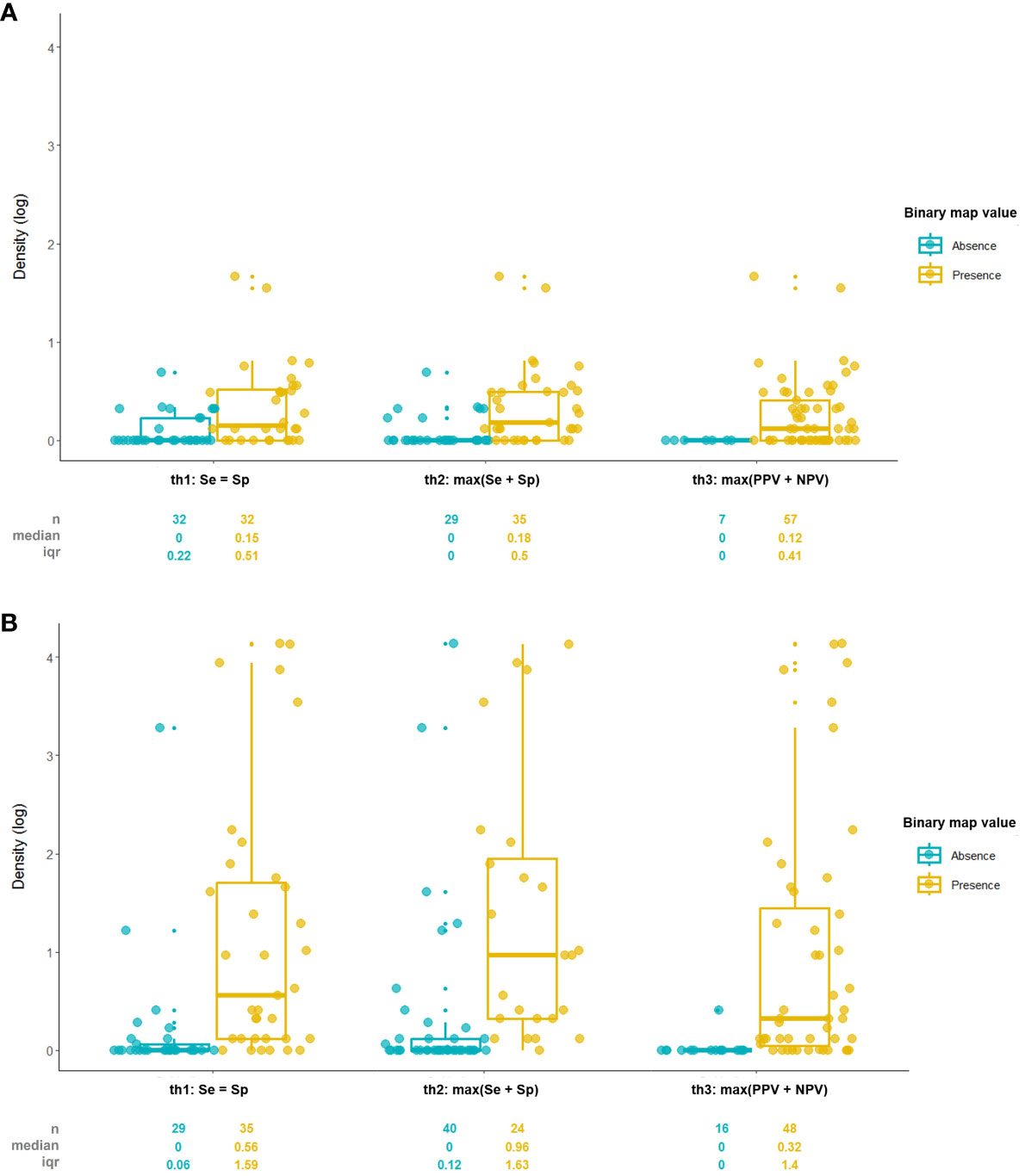
Figure 5 Scatterplots of suitability against density of (A) Japanese pine sawyer and (B) Sakhalin pine sawyer. The regression lines shown above represent the relationship fitted using 60th to 90th percentiles of quantile regression.
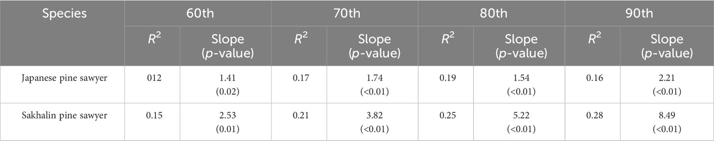
Table 1 Quantile regression of 60th, 70th, 80th, and 90th percentiles for the relationship between suitability and population density.
The result showed that the binary map created with the max(Se+Sp) threshold criteria was the most related to the density data with the highest Rb value, Se=Sp the second, and max(PPV+NPV) the least in both vectors (Table 2). Also the median density values in presence area created by max(Se+Sp) threshold were highest, Se=Sp the second, and max(PPV+NPV) the least (Figure 6). Every p-value of Rb was below 0.00, meaning the density and presence/absence are significantly correlated. While TSS (True Skill Statistic) calculated with the max(Se+Sp) threshold had the highest value for both models, TSS from the max(PPV+NPV) threshold was higher than the Se=Sp method in the SPS model.

Table 2 TSS and Rb coefficient for each threshold criteria.
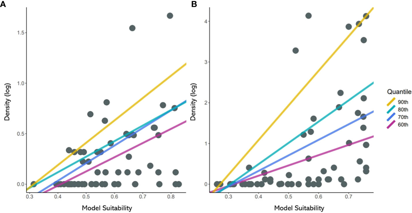
Figure 6 Comparison of density value between presence/absence areas divided by threshold criteria of (A) Japanese pine sawyer and (B) Sakhalin pine sawyer suitability map.
4 Discussion
PWD in South Korea is spreading despite the various control efforts (Korea Forest Service, 2022). Since the control period is determined by the vector, understanding the distribution and density of JPS and SPS is crucial (National Institute of Forest Science, 2016). This study is the first to predict the distribution of two vectors in South Korea using the Maxent model and investigate the relationship between suitability and population density of vectors. Quantile regression showed a consistent positive relationship between suitability and density in the upper quantile with a significant p-value. Presence/absence divided by max(Se+Sp) threshold criteria best discriminated the density value.
4.1 Characteristics of pine sawyer’s habitat suitability
The distribution of SPS was strongly influenced by the mean annual temperature. SPS requires 183-244 degree days above 10°C for larval development and adult emergence (Togashi et al., 1994) and is found in environmental conditions of mean annual temperature between 8.2 and 13.2°C (Kwon et al., 2006). The response curve of annual mean temperature also peaked between the range, successfully reflecting the temperature constraint of the species. The most important variable in JPS distribution was precipitation seasonality. Precipitation seasonality is the measure of the variation in monthly precipitation totals in a year, meaning a lower with smaller variability of precipitation (O’Donnell and Ignizio, 2012). JPS is predicted to distribute on the Southern region and coastlines of South Korea where precipitation seasonality is relatively low (Yoon et al., 2006), and elevation is below 1,050m above sea level where JPS is usually found (Kobayashi, 1988; Kishi, 1995). Also, JPS requires an air temperature of at least 21.3°C for oviposition to occur (Hanks, 1999), and the response curve of mean temperature of warmest quarter coincides with such requirements.
4.2 Relationships between the density of pine sawyers and their habitat suitability
Quantile regression showed a constant positive relationship between predicted suitability and density. The increasing trend of pseudo r square indicates that upper limit of suitability-density distribution explains the relationship better. Suitability value driven from the climatic data does not reflect the density of the species directly, but the data is related to the upper limits of density with prevalent unmeasured factors (Tôrres et al., 2012). This relationship between suitability, density and unmeasured factors is described as triangular constraint envelope (Austin, 2007), as suitability can be interpreted as carrying capacity of the density and there are unmeasured factors limiting the species population (VanDerWal et al., 2009).
The reason for the constantly increasing trend of pseudo r square is assumed that the baseline of the distribution and population of the insect is set by climate (Khaliq et al., 2014; Skendžić et al., 2021). And the temperature is one of the most important factors, as the insect metabolic rates, consumption, development, and survival rates are highly affected (Bale et al., 2002; Dukes et al., 2009). The selected climatic variables and response curves in the models well matched with the physiology and distribution of the Monochamus species (Kwon et al., 2006). However, the insect population is spatially and temporally diverse with population dynamics of high inter-annual variation (Wallner, 1987; Hassell et al., 1991). There could be many unmeasured factors causing a partial mismatch between suitability and density, such as detection limitations of the pheromone trap, biotic interactions, or weather (Birch, 1957; Guisan and Thuiller, 2005; Araújo and Luoto, 2007; Lee et al., 2018).
The limitation of SDMs with only climatic variables was obvious when in comparison with the population density. Past studies showed the importance of considering multiple factors such as biotic interaction or human influences in depicting the species distribution (Araújo and Luoto, 2007; Austin, 2007). Many low densities were found in survey areas with relatively high suitability, causing wedge-shape in points distribution and low pseudo r square in quantile regression. One of the variables that could strongly influence the density but was not considered is human influence. Many PWD controls are implemented in South Korea to stop the spread, including aerial insecticide spray (Kwon et al., 2011). Although there is a possibility that the survey locations were affected by such control, no recent geographic information about the control location was available. Such limitation of suitability was also found in previous studies. VanDerWal et al. (2009) compared the SDM suitability and local density of 69 vertebrates. Most species showed wedge-shaped points distribution, and quantile regression with upper quantile showed better prediction than the ordinary linear regression.
Past studies have tested the threshold selection and its effects on the accuracy assessment of SDM (Liu et al., 2005; Liu et al., 2011; Bean et al., 2012). We used three widely used thresholds to test if they could also distinguish the density by comparing the Rb value of biserial correlation. The Se=Sp threshold is selected as Jiménez Valverde (2012) stated the importance of Se and Sp value yield by Se=Sp threshold as it is closely related with the AUC. Max(Se+Sp) is selected as the threshold that maximizes the sum of the sensitivity and specificity, which will certainly result in the highest TSS value as the index is calculated as Se+Sp–1. TSS is based on sensitivity and specificity and is defined as the average net prediction success rate for presence and absence sites (Liu et al., 2011). It is considered one of the best model performance assessments to distinguish between presence and absence (Biggerstaff, 2000; Allouche et al., 2006). Max(PPV + NPV) is the threshold that minimizes the predictive errors, representing the proportion of incorrect predicted presences and absences. PPV and NPV act as the counterparts of Se and Sp; Se and Sp are the probability that a known site is correctly predicted, and PPV and NPV are the probability that the model correctly predicts an observation (Liu et al., 2009). PPV and NPV are more often used in image classification assessments than SDM, widely known as user accuracy (Hand, 2001).
Although it is not identical to the biserial correlation, the point-biserial correlation coefficient was used in SDM to find a correlation between the dichotomous presence/absence dataset and the predicted probability (Zheng and Agresti, 2000; Elith et al., 2006). Biserial correlation is used when the dichotomous variable is converted binary by certain criteria, as in this study, suitability value converted to presence/absence, but point-biserial correlation`s dichotomous variable is inherently binary (Sheskin, 2011). Unlike the expectation, the rank of the Rb value did not match with TSS accordingly, but the max(Se+Sp) threshold model had the highest TSS and the strongest relationship with the density with the highest Re. Also, the median density value in the presence site of the max(Se+Sp) threshold was highest among the three, even when there were more absence sites than the Se=Sp threshold model, proving to be the threshold with the best discrimination capacity. Our result was similar to the past studies of Jiménez-Valverde and Lobo (2007) and Liu et al. (2005) that stated max(Se+Sp) and Se=Sp as one of the best threshold criteria. Our study suggests that the max(Se+Sp) threshold and binary map created by its criteria are more likely to explain species density better.
4.3 Performance of the model
The validation AUC calculated with the presence/absence derived from the density data had a higher value over cross-validation AUC. Such result may due to a small number of density points for validation or due to the calculation difference between background points used in cross-validation and true absence points used in validation (Jiménez Valverde, 2012). The Dismo package, by default, uses all 10,000 background points used in training and validation to calculate the AUC (Radosavljevic and Anderson, 2014), while JPS only had 32 true absences and SPS 26. Despite the prevalent use of AUC in SDM assessment (Fielding and Bell, 1997), it cannot be calculated properly without the true absence because the ROC curve is plotted with the commission error, or 1 - specificity (Jiménez Valverde, 2012). In the case of using background points to calculate AUC, the model can easily have low commission error as the number of absence is much higher than the presence (Lobo et al., 2008). Thus, the validation AUC value calculated from presence/absence should assess the model better.
Although the maxent models had intermediate AUC, suitability value drawn from the model was capable of explaining the relationship between density. The statistical performance of the model does not always comply with the goodness of prediction. Similar research done by Tôrres et al. (2012) showed simple BIOCLIM explained the relationship between suitability and density best, surpassing machine learning algorithms with higher AUC. Maxent is capable of fitting non-linear functions and prone to overfitting, which could bias the result (Muscarella et al., 2014). Species response to climate is expected to be smooth and simple features (Holt, 2009). But complex model can capture non-climate processes that possess local microenvironment that make ecological interpretation difficult (Pulliam, 2000). Therefore constraining the complexity of model based on the study object is recommended (Elith and Graham, 2009; Merow et al., 2014). PWD have spread country wide and generality of the model is required to prioritize and schedule the vector control. In this study, from occurrence data to parameter settings, the models are simplified to discover hidden patterns between suitability and density.
5 Conclusion
SDM is widely used to describe the habitat suitability or distribution range of various species (Guisan and Thuiller, 2005; Elith and Leathwick, 2009). However, the relationship between habitat suitability and density is still under debate, although the knowledge of the distribution and density of forest pests is essential in its control (Barbosa et al., 2012). Nationwide vector density data achieved by the National Institute of Forest Science and local governments made it possible to test the correlation between SDM habitat suitability and the density of two vectors of pine wilt nematode. The quantile regression revealed the hidden relationship that usual regression could not (Dunham, 1996; Dunham et al., 2002). Presence/absence divided by max(Se+Sp) threshold criteria best discriminated the density value. This study showed a positive correlation between predicted SDM suitability and density data of two main vectors of PWD. This quantitative relationship will give reliability to SDM and may provide better use as a practical tool for PWD in risk analysis and selecting priority areas in control planning.
Data availability statement
The original contributions presented in the study are included in the article/Supplementary Material. Further inquiries can be directed to the corresponding author.
Author contributions
IK: Conceptualization, Methodology, Software, Writing – original draft. YN: Investigation, Writing – review & editing. SP: Data curation, Visualization, Writing – review & editing. WC: Conceptualization, Writing – review & editing. KC: Conceptualization, Supervision, Writing – review & editing. DK: Conceptualization, Writing – review & editing.
Funding
The author(s) declare financial support was received for the research, authorship, and/or publication of this article. This study was carried out with the support of “R&D Program for Forest Science Technology (Project No. 2019150B10-2323-0301)” provided by Korea Forest Service(Korea Forestry Promotion Institute). This work was supported by the Korea Environment Institute (KEI) through the research project "Development of Strategies for Environmental Policy Research Support Using Generative Artificial Intelligence-Based Large Language Models" (RR2023-15).
Conflict of interest
The authors declare that the research was conducted in the absence of any commercial or financial relationships that could be construed as a potential conflict of interest.
Publisher’s note
All claims expressed in this article are solely those of the authors and do not necessarily represent those of their affiliated organizations, or those of the publisher, the editors and the reviewers. Any product that may be evaluated in this article, or claim that may be made by its manufacturer, is not guaranteed or endorsed by the publisher.
Supplementary material
The Supplementary Material for this article can be found online at: https://www.frontiersin.org/articles/10.3389/fevo.2023.1305573/full#supplementary-material
References
Aiello-Lammens M. E., Boria R. A., Radosavljevic A., Vilela B., Anderson R. P. (2015). spThin: An R package for spatial thinning of species occurrence records for use in ecological niche models. Ecography. 38 (5), 541–545. doi: 10.1111/ecog.01132
Allouche O., Tsoar A., Kadmon R. (2006). Assessing the accuracy of species distribution models: prevalence, kappa and the true skill statistic (TSS). J. Appl. ecology. 43 (6), 1223–1232. doi: 10.1111/j.1365-2664.2006.01214.x
Araújo M. B., Cabeza M., Thuiller W., Hannah L., Williams P. H. (2004). Would climate change drive species out of reserves? An assessment of existing reserve-selection methods. Global Change Biol. 10 (9), 1618–1626. doi: 10.1111/j.1365-2486.2004.00828.x
Araújo M. B., Luoto M. (2007). The importance of biotic interactions for modelling species distributions under climate change. Global Ecol. Biogeography. 16 (6), 743–753. doi: 10.1111/j.1466-8238.2007.00359.x
Austin M. (2007). Species distribution models and ecological theory : A critical assessment and some possible new approaches. Ecological Modelling 200 (1-2), 1–19. doi: 10.1016/j.ecolmodel.2006.07.005
Bale J. S., Masters G. J., Hodkinson I. D., Awmack C., Bezemer T. M., Brown V. K., et al. (2002). Herbivory in global climate change research: direct effects of rising temperature on insect herbivores. Global Change Biol. 8 (1), 1–16. doi: 10.1046/j.1365-2486.2002.00451.x
Barbet-Massin M., Jiguet F., Albert C. H., Thuiller W. (2012). Selecting pseudo-ab sences for species distribution models: How, where and how many? Methods Ecol. Evolution. 3 (2), 327–338. doi: 10.1111/j.2041-210X.2011.00172.x
Barbosa F. G., Schneck F., Melo A. S. (2012). Use of ecological niche models to predict the distribution of invasive species: a scientometric analysis. Braz. J. Biol. 72, 821–829. doi: 10.1590/S1519-69842012000500007
Bean W. T., Stafford R., Brashares J. S. (2012). The effects of small sample size and sample bias on threshold selection and accuracy assessment of species distribution models. Ecography. 35 (3), 250–258. doi: 10.1111/j.1600-0587.2011.06545.x
Biggerstaff B. J. (2000). Comparing diagnostic tests: a simple graphic using likelihood ratios. Stat Med. 19 (5), 649–663. doi: 10.1002/(SICI)1097-0258(20000315)19:5<649::AID-SIM371>3.0.CO;2-H
Birch L. C. (1957). The role of weather in determining the distribution and abundance of animals. Cold Spring Harbor Symp. Quantitative Biol. 22 (0), 203–218. doi: 10.1101/sqb.1957.022.01.021
Booth T. H. (2022). Checking bioclimatic variables that combine temperature and precipitation data before their use in species distribution models. Austral Ecology. 47 (7), 1506–1514. doi: 10.1111/aec.13234
Boria R. A., Olson L. E., Goodman S. M., Anderson R. P. (2014). Spatial filtering to reduce sampling bias can improve the performance of ecological niche models. Ecol. Modelling. 275, 73–77. doi: 10.1016/j.ecolmodel.2013.12.012
Brown J. H. (1984). On the relationship beween abundance and distribution of species. Am. Naturalist. 124 (2), 255–279. doi: 10.1086/284267
Brown J. L. (2014). SDM toolbox: a python-based GIS toolkit for landscape genetic, biogeographic and species distribution model analyses. Methods Ecol. Evolution. 5 (7), 694–700. doi: 10.1111/2041-210X.12200
Brown J. H., Gupta V. K., Li B. L., Milne B. T., Restrepo C., West G. B. (2002). The fractal nature of nature: power laws, ecological complexity and biodiversity. Philos. Trans. R. Soc. London. Ser. B: Biol. Sci. 357 (1421), 619–626. doi: 10.1098/rstb.2001.0993
CABI. (2021). “Bursaphelenchus xylophilus,” in Invasive species compendium (Wallingford: CAB International). Available at: www.cabi.org/isc.
Cade B. S., Noon B. R. (2003). A gentle introduction to quantile regression for ecologists. Front. Ecol. Environment. 1 (8), 412–420. doi: 10.1890/1540-9295(2003)001[0412:AGITQR]2.0.CO;2
Cade B. S., Noon B. R., Flather C. H. (2005). Quantile regression reveals hidden bias and uncertainty in habitat models. Ecology. 86 (3), 786–800. doi: 10.1890/04-0785
Cade B. S., Terrell J. W., Schroeder R. L. (1999). Estimating effects of limiting factors with regression quantiles. Ecology. 80 (1), 311–323. doi: 10.1890/0012-9658(1999)080[0311:EEOLFW]2.0.CO;2
Choi W. I., Park Y. S. (2012). Dispersal patterns of exotic forest pests in South Korea. Insect Science. 19 (5), 535–548. doi: 10.1111/j.1744-7917.2011.01480.x
Dukes J. S., Pontius J., Orwig D., Garnas J. R., Rodgers V. L., Brazee N., et al. (2009). Responses of insect pests, pathogens, and invasive plant species to climate change in the forests of northeastern North America: what can we predict? Can. J. For. Res. 39 (2), 231–248. doi: 10.1139/X08-171
Dunham J. B. (1996). The population ecology of stream-living Lahontan cutthroat trout (Oncorhynchus clarki henshawi) (Reno: University of Nevada).
Dunham J. B., Cade B. S., Terrell J. W. (2002). Influences of spatial and temporal variation on fish-habitat relationships defined by regression quantiles. Trans. Am. Fisheries Soc. 131 (1), 86–98. doi: 10.1577/1548-8659(2002)131<0086:IOSATV>2.0.CO;2
Elith J., Graham C. H. (2009). Do they? How do they? WHY do they differ? on finding reasons for differing performances of species distribution models. Ecography. 32 (1), 66–77. doi: 10.1111/j.1600-0587.2008.05505.x
Elith J., Graham H., C. P., Dudík M., Ferrier S., Guisan A., et al. (2006). Novel methods improve prediction of species’ distributions from occurrence data. Ecography. 29 (2), 129–151. doi: 10.1111/j.2006.0906-7590.04596.x
Elith J., Kearney M., Phillips S. (2010). The art of modelling range-shifting species. Methods Ecol. evolution. 1 (4), 330–342. doi: 10.1111/j.2041-210X.2010.00036.x
Elith J., Leathwick J. R. (2009). Species distribution models: ecological explanation and prediction across space and time. Annu. Rev. ecology evolution systematics. 40, 677–697. doi: 10.1146/annurev.ecolsys.110308.120159
Elith J., Phillips S. J., Hastie T., Dudík M., Chee Y. E., Yates C. J. (2011). A statistical explanation of MaxEnt for ecologists. Diversity distributions. 17 (1), 43–57. doi: 10.1111/j.1472-4642.2010.00725.x
Elmendorf S. C., Moore K. A. (2008). Use of community-composition data to predict the fecundity and abundance of species. Conserv. Biol. 22 (6), 1523–1532. doi: 10.1111/j.1523-1739.2008.01051.x
Esri Inc. (2020). ArcGIS pro (Version 2.5) (California: Esri Inc.). Available at: https://www.esri.com/en-us/arcgis/products/arcgis-pro/overview.
Estay S. A., Labra F. A., Sepulveda R. D., Bacigalupe L. D. (2014). Evaluating habitat suitability for the establishment of Monochamus spp. through climate-based niche modeling. PloS One 9 (7), e102592. doi: 10.1371/journal.pone.0102592
Fielding A. H., Bell J. F. (1997). A review of methods for the assessment of prediction errors in conservation presence/absence models. Environ. Conserv. 24 (1), 38–49. doi: 10.1017/S0376892997000088
Franklin J. (2010). Mapping species distributions: spatial inference and prediction (Cambridge: Cambridge University Press).
Futai K. (2013). Pine wood nematode, bursaphelenchus xylophilus. Annu. Rev. Phytopathology. 51, 61–83. doi: 10.1146/annurev-phyto-081211-172910
Geier P. W. (1966). Management of insect pests. Annu. Rev. Entomology. 11 (1), 471–490. doi: 10.1146/annurev.en.11.010166.002351
Guillera-Arroita G., Lahoz-Monfort J. J., Elith J., Gordon A., Kujala H., Lentini P. E., et al. (2015). Is my species distribution model fit for purpose? Matching data and models to applications. Global Ecol. biogeography. 24 (3), 276–292. doi: 10.1111/geb.12268
Guisan A., Thuiller W. (2005). Predicting species distribution: Offering more than simple habitat models. Ecol. Letters. 8 (9), 993–1009. doi: 10.1111/j.1461-0248.2005.00792.x
Hand D. J. (2001). Measuring diagnostic accuracy of statistical prediction rules. Statistica Neerlandica. 55 (1), 3–16. doi: 10.1111/1467-9574.00153
Hanks L. M. (1999). Influence of the larval host plant on reproductive strategies of cerambycid beetles. Annu. Rev. Entomology. 44, 483–505. doi: 10.1146/annurev.ento.44.1.483
Hassell M. P., Comins H. N., Mayt R. M. (1991). Spatial structure and chaos in insect population dynamics. Nature. 353 (6341), 255–258. doi: 10.1038/353255a0
Hijmans R. J., Cameron S. E., Parra J. L., Jones P. G., Jarvis A. (2005). Very high resolution interpolated climate surfaces for global land areas. Int. J. Climatology. 25 (15), 1965–1978. doi: 10.1002/joc.1276
Hijmans R. J., Phillips S., Leathwick J., Elith J., Hijmans M. R. J. (2017). Package ‘dismo’. Circles. 9 (1), 1–68.
Holt R. D. (2009). Bringing the Hutchinsonian niche into the 21st century: Ecological and evolutionary perspectives. Proc. Natl. Acad. Sci. United States America 106 (SUPPL. 2), 19659–19665. doi: 10.1073/pnas.0905137106
Hutchinson G. E. (1959). Homage to Santa Rosalia or why are there so many kinds of animals? Am. Nat. 93 (870), 145–159. doi: 10.1086/282070
Jiménez Valverde A. (2012). Insights into the area under the receiver operating characteristic curve (AUC) as a discrimination measure in species distribution modelling. Global Ecol. Biogeography. 21 (4), 498–507. doi: 10.1111/j.1466-8238.2011.00683.x
Jiménez-Valverde A., Lobo J. M. (2007). Threshold criteria for conversion of probability of species presence to either–or presence–absence. Acta oecologica. 31 (3), 361–369. doi: 10.1016/j.actao.2007.02.001
Juliano S. A. (2007). Population dynamics. J. Am. Mosq. Control Assoc. 23 (2 Suppl), 265. doi: 10.2987/8756-971X(2007)23[265:PD]2.0.CO;2
Kareiva P. (1990). Population dynamics in spatially complex environments: theory and data. Philos. Trans. R. Soc. London. Ser. B: Biol. Sci. 330 (1257), 175–190. doi: 10.1098/rstb.1990.0191
Khaliq A. M., Javed M., Sohail M., & Sagheer M. (2014). Environmental effects on insects and their population dynamics. J. Entomology Zoology Stud. 2 (2), 1–7.
Kim J., Jung H., Park Y. H. (2016). Predicting potential distribution of Monochamus alternatus Hope responding to climate change in Korea. Korean J. Appl. entomology. 55 (4), 501–511. doi: 10.5656/KSAE.2016.11.0.053
Kobayashi F. (1988). The Japanese pine sawyer. Dynamics For. Insect Popul. 194, 431–454. doi: 10.1007/978-1-4899-0789-9_21
Koenker R., Bassett G. Jr. (1978). Regression quantiles. Econometrica: J. Econometric Society. 46 (1), 33–50. doi: 10.2307/1913643
Koenker R., MaChado J. A. F. (1999). Goodness of fit and related inference processes for quantile regression. J. Am. Stat. Assoc. 94 (448), 1296–1310. doi: 10.1080/01621459.1999.10473882
Kwon Y. (2022a). niek_2022 (Seocheon: National Institute of Ecology). Available at: https://www.gbif.org/occurrence/3444239880.
Kwon Y. (2022b). niek_2022 (Seocheon: National Institute of Ecology). Available at: https://www.gbif.org/occurrence/3444332858.
Kwon H. J., Jung J. K., Jung C., Han H., Koh S. H. (2018). Dispersal capacity of Monochamus saltuarius on flight mills. Entomologia Experimentalis Applicata. 166 (5), 420–427. doi: 10.1111/eea.12686
Kwon T. S., Lim J. H., Sim S. J., Kwon Y. D., Son S. K., Lee K. Y., et al. (2006). Distribution patterns of Monochamus alternatus and M. saltuarius (Coleoptera: Cerambycidae) in Korea. J. Korean Soc. For. Science. 95 (5), 543–550.
Kwon T. S., Shin J. H., Lim J. H., Kim Y. K., Lee E. J. (2011). Management of pine wilt disease in Korea through preventative silvicultural control. For. Ecol. Management. 261 (3), 562–569. doi: 10.1016/j.foreco.2010.11.008
Lee H. R., Lee S. C., Lee D. H., Jung M., Kwon J. H., Huh M. J., et al. (2018). Identification of aggregation-sex pheromone of the Korean Monochamus alternatus (coleoptera: Cerambycidae) population, the main vector of pine wood nematode. J. Economic Entomology. 111 (4), 1768–1774. doi: 10.1093/jee/toy137
Liu C., Berry P. M., Dawson T. P., Pearson R. G. (2005). Selecting thresholds of occurrence in the prediction of species distributions. Ecography. 28 (3), 385–393. doi: 10.1111/j.0906-7590.2005.03957.x
Liu C., White M., Newell G. (2009). Measuring the accuracy of species distribution models: a review. In Anderssen R. S., Braddock R. D., Newham L. T. H. (eds) 18th World IMACS Congress and MODSIM09 International Congress on Modelling and Simulation. Modelling and Simulation Society of Australia and New Zealand and International Association for Mathematics and Computers in Simulation, July 2009, pp. 4241–4247.
Liu C., White M., Newell G. (2011). Measuring and comparing the accuracy of species distribution models with presence–absence data. Ecography. 34 (2), 232–243. doi: 10.1111/j.1600-0587.2010.06354.x
Lobo J. M., Jiménez-Valverde A., Real R. (2008). AUC: a misleading measure of the performance of predictive distribution models. Global Ecol. Biogeography. 17 (2), 145–151. doi: 10.1111/j.1466-8238.2007.00358.x
Loiselle B. A., Howell C. A., Graham C. H., Goerck J. M., Brooks T., Smith K. G., et al. (2003). Avoiding pitfalls of using species distribution models in conservation planning. Conserv. Biol. 17 (6), 1591–1600. doi: 10.1111/j.1523-1739.2003.00233.x
Mamiya Y. (1972). Pine wood nematode, Bursaphelenchus lignicolus Mamiya and Kiyohara, as a causal agent of pine wilting disease. Rev. Plant Prot. Res. 5, 46–60.
Mamiya Y., Enda N. (1972). Transmission of Bursaphelenchus lignicolus (nematoda: Aphelenchoididae) by Monochamus alternatus (coleoptera: Cerambycidae). Nematologica 18 (2), 159–162. doi: 10.1163/187529272X00395
Matsuhashi S., Hirata A., Akiba M., Nakamura K., Oguro M., Takano K. T., et al. (2020). Developing a point process model for ecological risk assessment of pine wilt disease at multiple scales. For. Ecol. Management. 463, 118010. doi: 10.1016/j.foreco.2020.118010
Merow C., Smith M. J., Edwards T. C., Guisan A., Mcmahon S. M., Normand S., et al. (2014). What do we gain from simplicity versus complexity in species distribution models? Ecography. 37 (12), 1267–1281. doi: 10.1111/ecog.00845
Mota M. M., Futai K., Vieira P. (2009). “Pine wilt disease and the pinewood nematode, Bursaphelenchus xylophilus,” in Integrated management of fruit crops nematodes. Vol. 4 (Dordrecht: Springer), 253–274.
Muscarella R., Galante P. J., Soley-Guardia M., Boria R. A., Kass J. M., Uriarte M., et al. (2014). ENMeval: An R package for conducting spatially independent evaluations and estimating optimal model complexity for Maxent ecological niche models. Methods Ecol. Evolution. 5 (11), 1198–1205. doi: 10.1111/2041-210x.12261
National Geography Information Institute (2020). The national atlas of korea II (Sejong: Ministry of Land Infrastructure and Transport).
National Institute of Forest Science (2016). Analysis of damage patterns of pine wilt disease by tree species and improvement of control technology (Seoul: National Institute of Forest Science).
Nielsen S. E., Johnson C. J., Heard D. C., Boyce M. S. (2005). Can models of presence-absence be used to scale abundance? Two case studies considering extremes in life history. Ecography. 28 (2), 197–208. doi: 10.1111/j.0906-7590.2005.04002.x
O’Donnell M. S., Ignizio D. A. (2012). Bioclimatic predictors for supporting ecological applications in the conterminous United States. U.S Geological Survey Data Series. 691 (10), 4–9.
Padalia H., Srivastava V., Kushwaha S. P. S. (2014). Modeling potential invasion range of alien invasive species, Hyptis suaveolens (L.) Poit. in India: Comparison of MaxEnt and GARP. Ecol. informatics. 22, 36–43. doi: 10.1016/j.ecoinf.2014.04.002
Park C., Choi Y., Moon J. Y., Yun W. T. (2009). Classification of climate zones in South Korea considering both air temperature and rainfall. J. Korean Geographical Society. 44 (1), 1–16.
Pearce J., Ferrier S. (2001). The practical value of modelling relative abundance of species for regional conservation planning: a case study. Biol. Conserv. 98 (1), 33–43. doi: 10.1016/S0006-3207(00)00139-7
Pearson R. G. (2010). Network of conservation educators & Practitioners species’ Distribution modeling for conservation educators and practitioners. In Conserv. 3, 54–89.
Pearson R. G., Raxworthy C. J., Nakamura M., Townsend Peterson A. (2007). Predicting species distributions from small numbers of occurrence records: A test case using cryptic geckos in Madagascar. J. Biogeography 34 (1), 102–117. doi: 10.1111/j.1365-2699.2006.01594.x
Peterson A. T., Pape M., Soberon J. (2015). Mechanistic and correlative models of ecological niches. Eur. J. Ecology. 1 (2), 28–38. doi: 10.1515/eje-2015-0014
Peterson A., Soberón J., Pearson R., Anderson R., Martínez-Meyer E., Nakamura M., et al. (2012). Ecological niches and geographic distributions (MPB-49) (Princeton: Princeton University Press, New Jersey). doi: 10.1515/9781400840670
Phillips S. J., Anderson R. P., Dudík M., Schapire R. E., Blair M. E. (2017). Opening the black box: An open-source release of Maxent. Ecography. 40 (7), 887–893. doi: 10.1111/ecog.03049
Phillips S. J., Anderson R. P., Schapire R. E. (2006). Maximum entropy modeling of species geographic distributions. Ecol. modelling. 190 (3-4), 231–259. doi: 10.1016/j.ecolmodel.2005.03.026
Phillips S. J., Dudík M. (2008). Modeling of species distributions with Maxent: New extensions and a comprehensive evaluation. Ecography. 31 (2), 161–175. doi: 10.1111/j.0906-7590.2008.5203.x
Pulliam H. R. (2000). On the relationship between niche and distribution. Ecol. Lett. 3 (4), 349–361. doi: 10.1046/j.1461-0248.2000.00143.x
Radosavljevic A., Anderson R. P. (2014). Making better Maxent models of species distributions: Complexity, overfitting and evaluation. J. Biogeography. 41 (4), 629–643. doi: 10.1111/jbi.12227
Schröder H. K., Andersen H. E., Kiehl K. (2005). Rejecting the mean: Estimating the response of fen plant species to environmental factors by non-linear quantile regression. J. Vegetation Science. 16 (4), 373–382. doi: 10.1111/j.1654-1103.2005.tb02376.x
Sheskin D. J. (2011). Handbook of parametric and nonparametric statistical procedures. Fifth Edition (Boca Raton, Florida: CRC Press).
Shin S. C. (2008). “Pine wilt disease in Korea,” in Pine wilt disease. Eds. Zhao B. G., Futai K., Sutherland J. R., Takeuchi Y. (Tokyo: Springer), 26–32.
Skendžić S., Zovko M., Živković I. P., Lešić V., Lemić D. (2021). The impact of climate change on agricultural insect pests. Insects 12 (5), 440. doi: 10.3390/insects12050440
Tang X., Yuan Y., Li X., Zhang J. (2021). Maximum entropy modeling to predict the impact of climate change on pine wilt disease in China. Front. Plant Sci. 12. doi: 10.3389/fpls.2021.652500
Thomson J. D., Weiblen G., Thomson B. A., Alfaro S., Legendre P. (1996). Untangling multiple factors in spatial distributions: lilies, gophers, and rocks. Ecology. 77 (6), 1698–1715. doi: 10.2307/2265776
Togashi K., Jikumaru S., Taketsune A., Takahashi F. (1994). Termination of Larval Diapause in Monochamus saltuarius (Coleoptera : Cerambycidae) under Natural Conditions. J. Japanese Forestry Soc. 76, 30–34. doi: 10.11519/jjfs1953.76.1_30
Tôrres N. M., De Marco P., Santos T., Silveira L., de Almeida Jácomo A. T., Diniz-Filho J. A. F. (2012). Can species distribution modelling provide estimates of population densities? A case study with jaguars in the Neotropics. Diversity Distributions. 18 (6), 615–627. doi: 10.1111/j.1472-4642.2012.00892.x
VanDerWal J., Shoo L. P., Johnson C. N., Williams S. E. (2009). Abundance and the environmental niche: environmental suitability estimated from niche models predicts the upper limit of local abundance. Am. Naturalist. 174 (2), 282–291. doi: 10.1086/600087
Vignali S., Barras A. G., Arlettaz R., Braunisch V. (2020). SDMtune: An R package to tune and evaluate species distribution models. Ecol. Evolution. 10 (20), 11488–11506. doi: 10.1002/ece3.6786
Wallner W. E. (1987). Factors affecting insect population dynamics: differences between outbreak and non-outbreak species. Annu. Rev. Entomology. 32 (87), 317–340. doi: 10.1146/annurev.en.32.010187.001533
Wang W., Peng W., Liu X., He G., Cai Y. (2022). Spatiotemporal dynamics and factors driving the distributions of pine wilt disease-damaged forests in China. Forests. 13 (2), 261. doi: 10.3390/f13020261
Yi C. K., Byun B. H., Park J. D., Yang S. I., Chang K. H. (1989). First finding of the pine wood nematode, Bursaphelenchus xylophilus (Steiner et Buhrer) Nickle and its insect vector in Korea. Res. Rep. Forestry Res. Institute 38, 141–149.
Yoon H. J., Kim H. J., Yoon I. H. (2006). On the Study of the Seasonality Precipitatio over South Korea. J. Kor. Earth Sci. Soc. 27 (2), 149–158.
Yoon S., Jung J. M., Hwang J., Park Y., Lee W. H. (2023). Ensemble evaluation of the spatial distribution of pine wilt disease mediated by insect vectors in South Korea. For. Ecol. Management. 529, 120677. doi: 10.1016/j.foreco.2022.120677
Zhao B. G., Futai K., Sutherland J. R., Takeuchi Y. (2008). Pine wilt disease Vol. 17 (Tokyo: Springer), 459.
Keywords: quantile regression, pest management, pine wilt nematode, biserial correlation, Maxent, Monochamus spp.
Citation: Kim I, Nam Y, Park S, Cho W, Choi K and Ko DW (2024) Enhancing pest control interventions by linking species distribution model prediction and population density assessment of pine wilt disease vectors in South Korea. Front. Ecol. Evol. 11:1305573. doi: 10.3389/fevo.2023.1305573
Received: 02 October 2023; Accepted: 27 December 2023;
Published: 22 March 2024.
Edited by:
Margarida Espada, University of Évora, PortugalReviewed by:
Paulo A. V. Borges, University of the Azores, PortugalDaniel Scherrer, Swiss Federal Institute for Forest, Snow and Landscape Research (WSL), Switzerland
Copyright © 2024 Kim, Nam, Park, Cho, Choi and Ko. This is an open-access article distributed under the terms of the Creative Commons Attribution License (CC BY). The use, distribution or reproduction in other forums is permitted, provided the original author(s) and the copyright owner(s) are credited and that the original publication in this journal is cited, in accordance with accepted academic practice. No use, distribution or reproduction is permitted which does not comply with these terms.
*Correspondence: Dongwook W. Ko, dwko@kookmin.ac.kr