Theoretical Foundation for Pricing Climate-Related Loss and Damage in Infrastructure Financing

Abstract

This paper presents a novel theoretical framework for incorporating climate risks and adaptation investments into infrastructure debt pricing. Utilizing the Capital Asset Pricing Model (CAPM), the framework extends the conventional modeling of infrastructure project revenues and costs to include climate risk considerations. It proposes three climate-informed revenue and cost formulations: adjustmentment of mean and standard deviation, incorporation of extreme climate events via Pareto and Poisson distributions, and a climate-informed cost model that includes adaptation investment. The paper demonstrates the application of this model in pricing a loan for a Light Rail Transit project in Costa Rica, introducing the concepts of “flood risk premium” and “adaptation curves”. This study not only offers a novel lens through which to view infrastructure investment under climate uncertainty but also sets the stage for transformative policy and practice in financial risk assessment, encouraging a shift towards more sustainable and resilient infrastructure development.

1. Introduction

While the annual financing needed to adapt infrastructure to the impact of climate change is estimated sometimes in the trillions of dollars, such investment in adaptation has been slow to materialize. Investment in adaptation is still perceived as an additional cost to infrastructure projects that does not translate into tangible benefits. Such an assumption might not always be correct. The logic is simple: an infrastructure exposed to climate risks should have a higher cost of capital reflecting these risks, and adaptation, should lower the cost of capital as it lowers the risk. The return on adaptation investment could be quantified if the resulting avoided loss and damage was to be included in the pricing of cost of capital for a project.

It is therefore possible to conclude that one of the barriers to adaptation investment is analytical. It may be due to the lack of a theoretical framework allowing a simple pricing of climate risk, and adaptation measures, in financing operations. While significant literature has addressed infrastructure exposure to climate risks, few focused on modelling their impact on infrastructure’s cost of capital. Despite growing data availability on climate risk exposure, the integration of this information into financing operations remains a challenge, as noted by the 2023 United Nations Environmental Program. This paper aims at suggesting a theoretical foundation incorporating climate risks in infrastructure debt pricing.

I start by setting the baseline theoretical framework for the estimation of interest rates on debt to infrastructure projects based on the Capital Asset-Pricing Model (CAPM) and following (Wibowo 2006). Wibowo (2006) models infrastructure projects’ revenues following a normal distribution and their costs following a linear function of fixed and variables costs. I augment this model by updating the formulation of revenues and costs to incorporate climate risk.

I propose three types of climate-informed formulations of revenues. The first is based on the adjustment of the mean and standard deviation of revenues to account for variations linked to climate risk. Since the normal distribution does not capture extreme climate events, I suggest integrating extreme climate events through Pareto and Poisson distributions.

I also suggest a novel climate-informed formation of costs. I model increases in costs as a Poisson distribution and include adaptation investment. I introduce the concept of “adaptation curve”, to be distinguished from damage curves, and demonstrate that the use of a logistic function is appropriate to model adaptation. I then apply the theoretical foundation to price a ten-year loan to a Light Rail Transit (LRT) project in San José, Costa Rica, using publicly available financial information. I select flood as a climate risk and fit each of the distributions, Normal, Pareto, and Poisson, for revenues and costs using publicly available climate data.

I first estimate the baseline value of the interest rate on the loan without integrating flood risk information. I then estimate new interest rates for each model and determine a “flood risk premium” by comparing the new interest rate to the baseline.

The theoretical foundation discussed in this paper, grounded in the Capital Asset Pricing Model (CAPM), provides a practical method for pricing climate risk in infrastructure project financing. However, the model’s outcomes significantly differ depending on whether climate risks are incorporated through revenue adjustments, cost adjustments, or both, and whether adaptation measures are considered. The value of the flood risk premiums I find vary between 2 and 11 basis points.

Key considerations in the application of this theoretical model involve decisions on whether to integrate climate risks into revenue or cost calculations or both, influenced by factors such as revenue models and existing risk management mechanisms. For example, in projects with guaranteed revenue mechanisms such as Power Purchase Agreements, climate hazards might not affect revenues directly, while projects relying on market-based revenues may need a more in-depth analysis of climate impacts on revenue. Similarly, for cost-related considerations, existing insurance and risk transfer mechanisms can influence whether climate risks need to be reflected in pricing.

The choice of model also depends on the nature of climate hazards and data availability. Projects exposed to chronic hazards might require a model focusing on mean and variance changes, while those facing acute hazards might use a Pareto or Poisson-based approache. The paper also highlights data-related challenges, especially for greenfield projects, and suggests using data from similar existing projects as a baseline.

The paper distinguishes itself by developing and applying a novel theoretical framework that extends the Capital Asset Pricing Model (CAPM) to explicitly incorporate climate risks and adaptation investments into infrastructure debt pricing. Unlike existing literature that has primarily focused on the general impact of climate risks on infrastructure or the financial implications of such risks, this study introduces unique elements—namely, the ‘flood risk premium’ and ‘adaptation curves’. These concepts provide a more nuanced understanding of how climate risks can be quantified and integrated into the financial models used by institutions, offering a practical approach to incentivizing climate-resilient infrastructure projects. Without such a pricing approach, financial institutions have no incentive to reward climate-resilient projects with a lower cost of capital.

2. Motivations and Research Questions

The climate finance literature has made significant progress over the last years in collecting evidence on the effect of climate risk on prices across asset classes (Giglio et al. 2021). Frameworks were developed linking physical climate risks, firm revenues and cost structures (Bolton et al. 2020; Campiglio et al. 2023). However, a critical examination reveals a notable gap: a detailed focus on the micro-level implications of climate risk for individual infrastructure project financing remains underexplored.

Although important research has studied infrastructure exposure to climate risks (Stewart and Deng 2015; Kim et al. 2017; Gupta et al. 2018), only a fraction focused on the impact of climate risk on infrastructure cost of capital (Assab 2023a, 2023b). Much of the climate finance literature has focused on the macro-financial implications of climate risk for other classes (Karydas and Xepapadeas 2022). This oversight underscores a critical gap in our collective understanding and application of climate risk assessments in infrastructure financing.

Gaps remain in terms of micro-understanding at the level of individual infrastructure project financing. Such micro-level understanding is important to enable the financial sector to unlock the billions in adaptation investment needed to mitigate climate change (Dodman 2009; Fankhauser 2010; Hughes et al. 2010; Narain et al. 2016). In et al. (2021) and Luo et al. (2023), for instance, initiated such work on the micro-level implications of climate risk for electricity generation infrastructure.

Both (In et al. 2021) and (Luo et al. 2023) clarify the mechanisms through which physical climate risks can reduce revenues for energy generation projects. In et al. (2021) show that these risks can have an impact on financial performance through increases in costs due to damages from extreme events.

The literature often overlooks the nuanced ways in which adaptation and resilience measures can mitigate these financial impacts. The few existing studies that touch upon adaptation (Assab 2023a; Hong et al. 2023; Kelly and Molina 2023) tend to approach it tangentially, without integrating it into a robust theoretical framework for financial decision-making.

In relation to asset-pricing theory, the theoretical foundation linking micro-level frameworks to the macro-level climate finance literature still needs to be strengthened. Such a theoretical foundation should allow a more systematic integration of the uncertainties over the future trajectory of climate risk as well as the effectiveness of climate adaptation measures in infrastructure financing decisions. It should leverage pricing techniques used in practice by the financial industry. The 2023 United Nations Environmental Program (UNEP) landscape of climate risk tools notes that although there is an increase in data availability on climate risk exposure of assets, finance practitioners still struggle to incorporate insights from these tools in their financing operations (Carlin et al. 2023).

This paper seeks to bridge these gaps by proposing a novel theoretical framework that not only accounts for the direct impact of climate risk on infrastructure project financing but also systematically incorporates adaptation investments into debt pricing. By extending the Capital Asset Pricing Model (CAPM) to include climate risk adjustments and introducing innovative concepts like the “flood risk premium” and “adaptation curves”, this study offers a comprehensive solution to the methodological limitations identified in the existing literature.

Adaptation is seldom discussed in the climate finance literature. Only a few empirical and theoretical studies provide evidence that adaptation measures reduce climate-financial risks (Assab 2023a; Hong et al. 2023; Kelly and Molina 2023). Therefore, a robust theoretical foundation should also integrate adaptation and resilience considerations. Our approach provides a practical tool for financial institutions to evaluate and incentivize climate-resilient infrastructure projects, thereby addressing the critical need for a more nuanced understanding of climate risk in infrastructure financing.

This paper intends to bridge these analytical and methodological gaps by answering the following two questions:

• What theoretical foundation is suitable to incorporate climate risks in the pricing of debt for infrastructure projects?
• Can this theoretical foundation incorporate different models of revenue and cost, as well as allow discussions on adaptation measures?

This paper focuses on the pricing of infrastructure debt. Debt represents the majority of private sector financing for infrastructure. According to the 2023 Infrastructure Monitor,1 debt represents 81 percent of total infrastructure financing. The theoretical foundation presented in this paper is transferable to the study of climate risk impact on infrastructure equity returns, especially given the fact that climate risk considerations are factored in through project revenues and costs.

3. Theoretical Foundation

3.1. CAPM-Based Pricing of Infrastructure Debt

The Capital Asset Pricing Model (CAPM) is a much-debated asset pricing model in terms of relevance, accuracy, and sophistication (Jagannathan and McGrattan 1995; Fama and French 1996; Levy 2010). Yet, it is still the main model used to make infrastructure investment and financing decisions, as well as in estimating the cost of debt and equity (Wibowo 2006; Sarmento and Oliveira 2018; Savoia et al. 2019). It is therefore a good starting point for a theoretical framework that intends to mainstream climate risk pricing in infrastructure financing decisions.

I build on the work developed by (Dias and Ioannou 1995; Wibowo 2006) who developed a CAPM-based valuation method for infrastructure project debt and equity.

I adopt the methodology formulated by (Wibowo 2006) to integrate physical climate risk in infrastructure asset valuation. I consider a basic infrastructure financing setting where a Special Purpose Vehicle (SPV) is created and the financial performance of the project depends mainly on its revenues and costs. In this section, I start by explaining how (Wibowo 2006) models infrastructure debt value and pricing (expressed through the interest rate). I then augment the model to account for climate risks.

Wibowo (2006) considers that infrastructure debt and equity are risky assets and that therefore the return on these assets follows Equation (1) derived from the CAPM:

$$E(\tilde{r})=\frac{E(\widetilde{X_1)}}{X}-1$$

(1)

where r is the return on asset, E is the expected value of returns, X₁ is the end-of-period value of the asset (debt or equity), and X is the asset’s present value. In this context, when referring to assets, we mean financial assets, meaning debt or equity, and not physical assets such as the infrastructure itself. $\widetilde{X_1}$ and X are formulated as follows:

$$X=\frac{E(\widetilde{{\displaystyle X_1}})-\lambda \mathrm{cov}(\widetilde{{\displaystyle X_1}};{\widetilde{{\displaystyle r}}}_m)}{(1+rf)}$$

(2)

where

$$\lambda =\frac{E({\widetilde{{\displaystyle r}}}_m)-{{\displaystyle r}}_f}{{{\displaystyle \sigma }}_m^2}$$

(3)

In the above Equations (2) and (3), r_m is the expected market return, r_f the risk-free rate, and σ_m the market volatility.

In the (Wibowo 2006) infrastructure debt valuation framework, debt is a risky asset. Projects are financed through an SPV structure and the party providing the debt (bank loans, capital markets bonds, etc.) do not have any recourse to the parent firm of the infrastructure company. The debt repayment is solely dependent on the project revenues and default occurs when the revenues are below the required debt service.

Let us assume that $\widetilde{{\displaystyle R}}$ is the operating revenue for the project and d₁ the promised debt service to the debt providers. $\widetilde{{\displaystyle R}}$ is assumed to obey a normal distribution with E($\widetilde{{\displaystyle R}}$) and σ_R to be its mean and standard deviation. The project cost comprises a fixed cost and variable cost proportional to revenues following Equation (4) based on (Dias and Ioannou 1995).

$$\widetilde{{\displaystyle C}}={{\displaystyle c}}_v\widetilde{{\displaystyle R}}+{{\displaystyle c}}_f$$

(4)

In order to have a full picture on the cost, we need to model the costs associated with a bankruptcy event that can be due to legal and administrative costs, sales of fixed assets and inventories, and other costs. We adopt the formulation of cost bankruptcy by (Kim 1978; Wibowo 2006) following Equation (5) where $\widetilde{{\displaystyle V}}$ is the project’s net operating revenue, revenue minus cost, described in Equation (6):

$$\widetilde{{\displaystyle B}}={{\displaystyle b}}_v\widetilde{{\displaystyle V}}+{{\displaystyle b}}_f$$

(5)

where

$$\widetilde{{\displaystyle V}}={\displaystyle (1-c_v)}\widetilde{{\displaystyle R}}-{{\displaystyle c}}_f$$

(6)

To value the debt, we need to understand its risk and express it vis-à-vis potential bankruptcy events. Following the notation by (Wibowo 2006), let us assume $\widetilde{{\displaystyle D_1}}$ as the payment to debt investors. In an event of bankruptcy, the value of the project’s payment to the debt investor is the operating income minus any bankruptcy costs following Equation (7).

$$\widetilde{{\displaystyle D_1}}=\widetilde{{\displaystyle V}}-\widetilde{{\displaystyle B}}$$

(7)

This allows one to determine two extreme cases: (i) the best case scenario, in which the debt investors receive a full payment of the promised debt service, and (ii) the worst case scenario, where the debt investors receive no payments.

Following (Wibowo 2006), we call a the revenue level that corresponds to a full payment of debt service to investors corresponding to $\widetilde{{\displaystyle V}}$ = d₁ and described in (8). We call b the revenue level at which investors do not receive any payments corresponding to $\widetilde{{\displaystyle V}}=\widetilde{{\displaystyle B}}$ and described in (9).

$$a=\frac{{{\displaystyle d}}_1+{{\displaystyle c}}_f}{1-{{\displaystyle c}}_v}$$

(8)

and

$$b=\frac{{{\displaystyle b}}_f+{{\displaystyle c}}_f(1-{{\displaystyle b}}_v)}{(1-{{\displaystyle c}}_v)(1-{{\displaystyle b}}_v)}$$

(9)

Based on the above, it then becomes possible to draw a general formulation of the payment to debt investors, D₁, following Equations (10)–(12):

$$\widetilde{{\displaystyle D_1}}={{\displaystyle d}}_1\mathrm{if}\widetilde{{\displaystyle R}}\ge a$$

(10)

$$\widetilde{{\displaystyle D_1}}=(1-b_v)[(1-c_v)\widetilde{{\displaystyle R}}-c_f]-b_f\mathrm{if}b\le \widetilde{{\displaystyle R}}<a$$

(11)

$$\widetilde{{\displaystyle D_1}}=0\mathrm{if}\widetilde{{\displaystyle R}}<b$$

(12)

At this stage, we have all the elements to determine the present value of the debt following the CAPM model and Equation (1). In accord with (Wibowo 2006), the detailed computation of the expected debt service and the covariance between the debt service and the market returns is as follows.

Expected payment to debt investors, E($\widetilde{{\displaystyle D_1}}$), is:

$$\begin{array}{c}E(\widetilde{{\displaystyle D_1}})=d_1[1-F_R(a)]\\ +(1-b_v)(1-c_v)\text{{}E(\widetilde{{\displaystyle R}})[F_R(a)-F_R(b)]\\ +{\sigma }_R^2[f_R(b)-f_R(a)]\}-[(1-b_v)c_f+b_f][F_R(a)-F_R(b)]\end{array}$$

(13)

where F_R is the operator of the cumulative normal distribution function and f_R the operator of probability normal distribution function.

The present value of debt D can be written as:

$$D=\frac{1}{1+{{\displaystyle r}}_f}[E\left(D_1\right)-\lambda \mathrm{cov}(D_1,r_m)]$$

(14)

Therefore, following Equation (1), the cost of debt, expressed as the interest rate of the debt (loan or bond) i, is given by:

$$i=\frac{{{\displaystyle d}}_1}{D}-1$$

(15)

3.2. Modelling Loss and Damage Due to Climate Hazards

Physical climate risks resulting from hazards such as floods, hurricanes, or extreme temperature can affect the financial performance of infrastructure projects via losses of revenues due to service interruption and increases in costs due to physical damage (Assab 2023a, 2023b).

In this section, I start by using three models for incorporating climate risk in the formulation of $\widetilde{{\displaystyle R}}$, the operating revenue. The baseline model assumes that $\widetilde{{\displaystyle R}}$ follows a normal distribution. First, I propose an incorporation of climate risk by altering the mean and variance of the normal distribution. I then suggest an alternative method consisting of augmenting the expression of $\widetilde{{\displaystyle R}}$ with a factor depending on climate events. I then model the climate events’ frequency and severity as Pareto and Poisson distributions, respectively, chosen for their well-documented ability to model extreme values and rare events, effectively capturing the irregular and significant impact of climate hazards on infrastructure projects.

I then present a model to incorporate climate risk in the project cost $\widetilde{{\displaystyle C}}$. For modelling the impact of climate risk on costs, I focus on the role of adaptation. I assume that climate risks increase costs incrementally by a factor proportionate to the damage resulting from climate events. I suggest an innovative formulation of the dependency between damage and adaptation investment, highlighting the pragmatic choice of this formulation to reflect the realistic impact of adaptation measures on mitigating climate risk, grounded in empirical evidence and theoretical insights from climate resilience studies.

In the rest of the section, I develop each of the components of the model in detail. I then apply this model to price a loan for a Light Rail Transit project in Costa Rica. I discuss each of the assumptions of the model in the case study.

3.2.1. Normal Distribution with Updated Mean and Variance

I model the operating revenue $\widetilde{{\displaystyle R}}$ as a normal distribution, and reflect climate consideration on revenues through altering the mean value and variance of $\widetilde{{\displaystyle R}}$. Increases in the frequency and severity of climate events can both decrease the average value of revenues and increase their volatility resulting in different values for E($\widetilde{{\displaystyle R}}$) and ${\sigma }_R^2$.

$$\widetilde{{\displaystyle R}}~N(E(\widetilde{{\displaystyle R}}),{\sigma }_R^2)$$

(16)

3.2.2. Climate Damage as a Pareto Distribution

Operating revenue $\widetilde{{\displaystyle R}}$ can also be adjusted for the impact of physical climate hazards following Equation (17), where ${\widetilde{{\displaystyle R}}}_{\mathrm{base}}$ is the base operating revenue without the impact of a climate hazard. D represents the proportion of revenue lost due to climate risk. The total revenue considering the impact of climate risk is modeled as:

$$\widetilde{{\displaystyle R}}={\widetilde{{\displaystyle R}}}_{\mathrm{base}}\times (1-D)$$

(17)

The damage factor due to climate risk, D, follows a Pareto distribution. The Pareto distribution is chosen because it models the ‘heavy-tailed’ nature of climate risk damages, representing the small probability but high impact of extreme climate events, aligning with observed patterns of climate-induced damages. Thus,

D ~ Pareto(x_m, α)

(18)

where x_m is the scale parameter (minimum value) and α is the shape parameter. The Probability Density Function of the Pareto distribution is given by:

$$f(x;x_m,\alpha )=\frac{\alpha x_m^{\alpha }}{x^{\alpha +1}} \mathrm{for} x\ge x_m,\alpha >0$$

(19)

The Cumulative Distribution Function of the Pareto distribution is:

$$F(x;x_m,\alpha )=1-\frac{x_m^{\alpha }}{x} \mathrm{for} x\ge x_m$$

(20)

The mean of the Pareto distribution is:

$$\mathrm{Mean}=\frac{\alpha x_m}{\alpha -1} \mathrm{for} \alpha >1$$

(21)

The variance of the Pareto distribution is:

$$\mathrm{Variance}=\frac{x_m^2\alpha }{{(\alpha -1)}^2(\alpha -2)} \mathrm{for} \alpha >2$$

(22)

3.2.3. Climate Hazard Occurrence as a Poisson Distribution

Operating revenue $\widetilde{{\displaystyle R}}$ can also be adjusted for the impact of physical climate hazards following Equation (23) where the occurrence of climate events is assumed to follow a Poisson Distribution.

$${\tilde{R}}_t=R_{\mathrm{b}\mathrm{a}\mathrm{s}\mathrm{e}}\times \left(1-\sum _{i=1}^{N_t}{\mathrm{S}\mathrm{e}\mathrm{v}\mathrm{e}\mathrm{r}\mathrm{i}\mathrm{t}\mathrm{y}}_i\right)$$

(23)

The Poisson distribution is a discrete probability distribution that expresses the probability of a given number of events occurring in a fixed interval of time or space. It is selected for its effectiveness in modeling the frequency of independent events within a given period, making it particularly suitable for quantifying the occurrence of climate hazards over time. It is characterized by the following probability mass function (PMF):

$$P(X=k)=\frac{\lambda k_e-\lambda }{k!}$$

(24)

where:

• X is the random variable representing the number of events;
• k is the number of occurrences of an event (non-negative integer);
• λ (lambda) is the average number of events per interval;
• e is Euler’s number, approximately equal to 2.71828;
• k! (k factorial) is the product of all positive integers up to k.

In the Poisson distribution, both the mean and the variance are equal to λ.

In Equation (23), ${\widetilde{{\displaystyle R}}}_{base}$ is the base operating revenue without the impact of the climate hazard, N represents the number of climate events in the period modeled by a Poisson distribution, and Severity_i denotes the severity of each climate hazard event.

The number of climate events N_t follows a Poisson distribution with a rate parameter λ:

N_t ~ Poisson(λ)

(25)

3.2.4. Climate Impact on Costs and Adaptation Needs

I consider the damage due to climate risk as a variable cost that occurs at a frequency that follows a Poisson distribution and that causes an average damage E(ClimateDamage). c_vbase is the baseline value of variable costs to which a damage due to climate risk is added following Equation (26).

c_v = c_vbase × (1 + Poisson(λ) × ExposureFactor × E(ClimateDamage))

(26)

The exposure factor, ExposureFactor, is the rate to which the infrastructure is exposed to climate risk and is between 0 and 1. The value 0 corresponds to the case where the infrastructure is fully adapted to the climate risk and where the climate event does not lead to any damage. The value 1 is the case where the infrastructure is not adapted to any exposed to climate risk and where it is fully damaged when a climate event occurs. Exposure to climate risks depends on the nature of the infrastructure as well as the investment in place to reduce climate risks. I refer to the investments as a single “adaptation investment”, calling the variable AdaptInvestment, and add it as a fixed cost to the project, since the presence of a climate risk means that the project sponsors need to invest risk mitigation measures.

c_f = c_f base + AdaptInvestment

(27)

$$\mathit{ExposureFactor}=\frac{1}{1+\delta \times \mathrm{e}\mathrm{x}\mathrm{p}\left(\gamma \mathrm{A}\mathrm{d}\mathrm{a}\mathrm{p}\mathrm{t}\mathrm{I}\mathrm{n}\mathrm{v}\mathrm{e}\mathrm{s}\mathrm{t}\mathrm{m}\mathrm{e}\mathrm{n}\mathrm{t}\right)}$$

(28)

The question is: what is the best mathematical formulation to capture the relationship between exposure to climate risk, ExposureFactor, and adaptation investment, AdaptInvest?

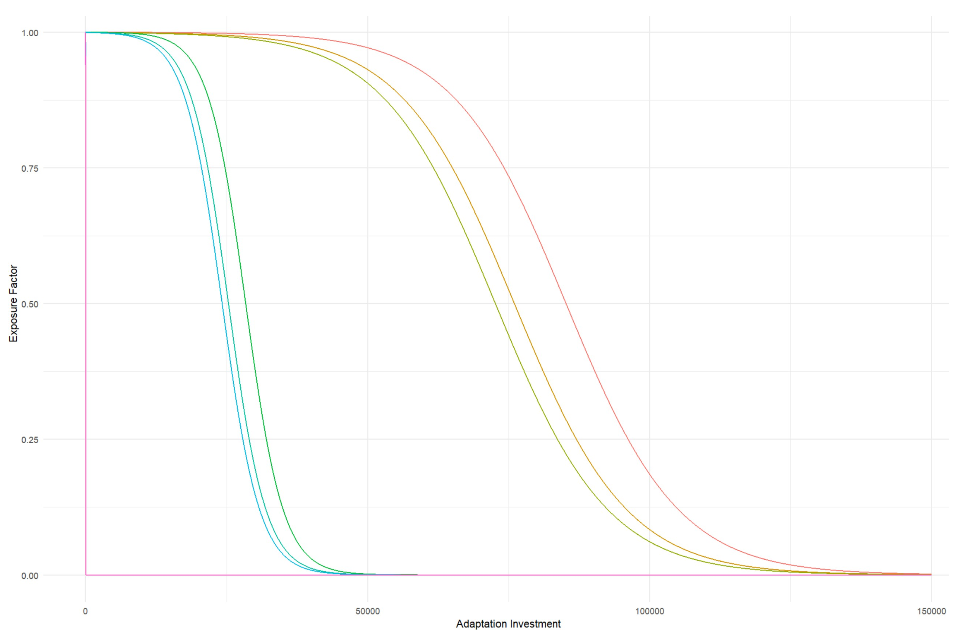
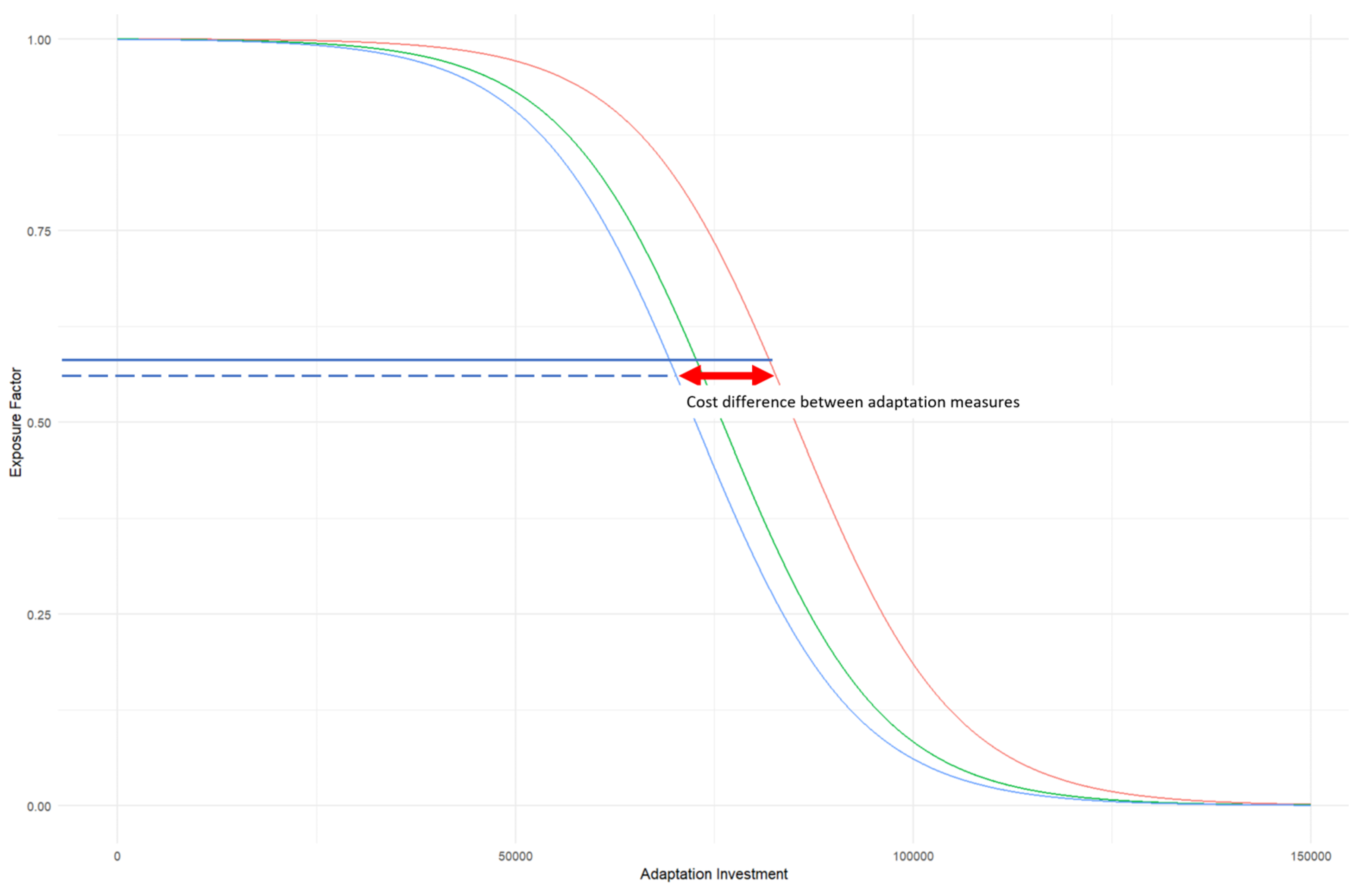
I suggest that this relationship follows a logistic function as described in Equation (28), which accurately reflects the diminishing returns of adaptation investments over time. First, the value of ExposureFactor is between 0 and 1. Then, there is a negative relationship between the exposure factor and investment. The higher the adaptation investment, the lower the exposure factor, and therefore, the lower the damage due to the extreme event. The exact nature of this relationship will however depend on the type of adaptation measures and the type of infrastructure, as well as the associated technical parameters. The logistic function is an ideal framework as it allows the calibration of this relationship using the variables δ and γ. Figure 1 show illustrations of the logistic function linking AdaptInvestment and ExposureFactor for different values of δ and γ. In other words, Figure 1 shows that for a given adaptation investment, it is possible to achieve various degrees of exposure depending on the value of δ and γ, i.e., the nature of adaptation measures.

In the next section, I discuss this theoretical foundation using the case study of a real investment project.

4. Application of the Model to Pricing Flood Risk in a Loan to San Jose Costa Rica Metro Line Project

In order to illustrate the proposed approach, I apply it to the pricing of a loan for the electric Light Rail Transit (LRT) system project in San Jose’s Great Metropolitan Area (GAM) in Costa Rica. It is an 85 km double-track LRT system, powered through renewable electricity that is aimed at reducing Costa Rica’s transport sector green house gas emissions as well as inefficiencies in the public transport system.

The San Jose LTR project was chosen because it was financed by the Green Climate Fund (GCF) in its 29 June 2021 Board meeting2. All the project’s documentation is publicly available online including technical analysis such the project’s Environmental Impact Assessment (EIA), risk assessment, and financial and economic assessment. Thanks to these documents, I was able to extract accurate information to serve as assumptions for the pricing of the loan. The project’s financial information I use was extracted from the document “Fourth Report: Economic and Financial Survey” and the relevant environmental information was extracted from “Second Report: Preliminary Environmental Study” (IDOM CONSULTING 2020).

In this section, I start by estimating the baseline interest rate for a 10-year loan to the GAM LRT. I then apply each of the modelling approaches I described previously to determine the interest rate including climate risk. For each approach, I compare the climate-informed interest rate to the baseline interest rate to estimate the premium associated with the project’s exposure to climate risk.

4.1. Baseline Estimation of the Loan Pricing

According to the project documentation, the risk-free rate r_f in Costa Rica was determined to be 10.55% based on the arithmetic average of the 10-year government bond between 2014 and 2019. The market return r_m was estimated based on the geometric average returns of the S&P 500 Index between 1970 and 2019 at around 8%.

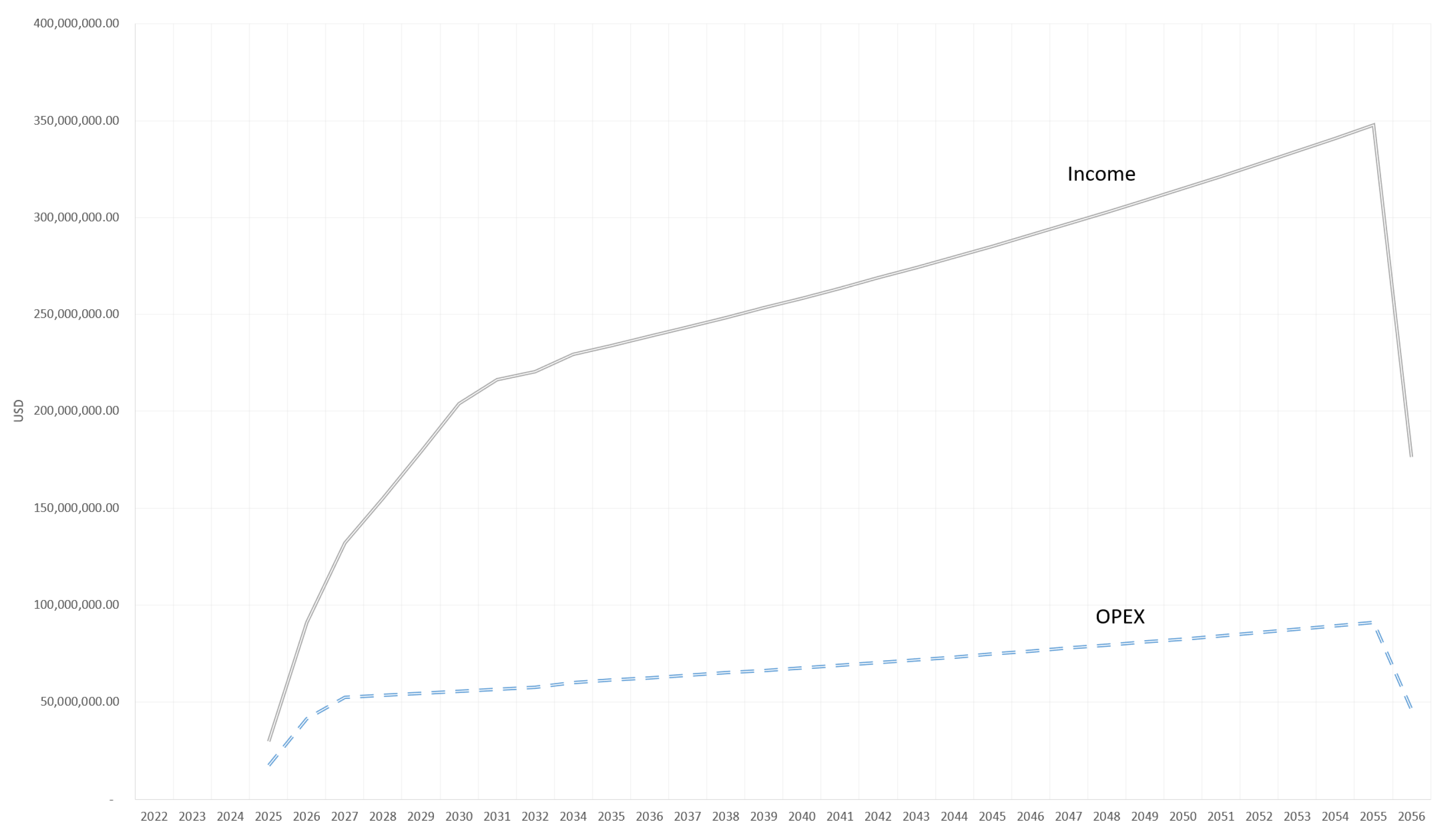
The financial modelling of the GAM LRT project estimates operating revenue between 2025 and 2056 for three scenarios: a baseline scenario, an optimistic scenario, and a worst-case scenario. I adopt the baseline operating revenue scenario shown in Figure 2 for the analysis. The expected revenue E($\widetilde{{\displaystyle R}}$) is USD 7.668 billion with a standard deviation σ_R of USD 75 million.

The cost $\widetilde{{\displaystyle C}}$ in the pricing model refers to operating cost of the project, OPEX, described in Figure 2. Using the project’s cash-flow statements, I perform an OLS regression in order to determine the variable component of costs c_v and fixed component c_f as described in Equation (4). The regression analysis is described in

Table 1. Determination of cost components.

	Dependent Variable
	OPEX
Income	0.210 *** (0.008)
Constant	15,121,669.000 *** (2,175,316.000)
Observations	31
Adjusted R2	0.954

Note: p-values described in parenthesis *** p < 0.01.

.

Based on the results of the regression analysis in Table 1, I estimate the value of c_v at 0.2 and the value of c_f at USD 15 million per year.

In absence of data on bankruptcy costs, I take a conservative stance and assume that the variable cost of bankruptcy b_v to be equal to 1. This means that in case of bankruptcy, all the project’s operating revenue will be used to cover the bankruptcy costs. I assume the fixed cost corresponding to administrative costs of bankruptcy b_v to be USD 2 million.

The project’s total investment cost is USD 1.85 billion (IDOM CONSULTING 2020) of which 75% was financed through debt. I therefore estimate d₁ at USD 1389 million.

Based on this financial project information, I price a 10-year loan for this project at a baseline interest rate i of 9.2%.

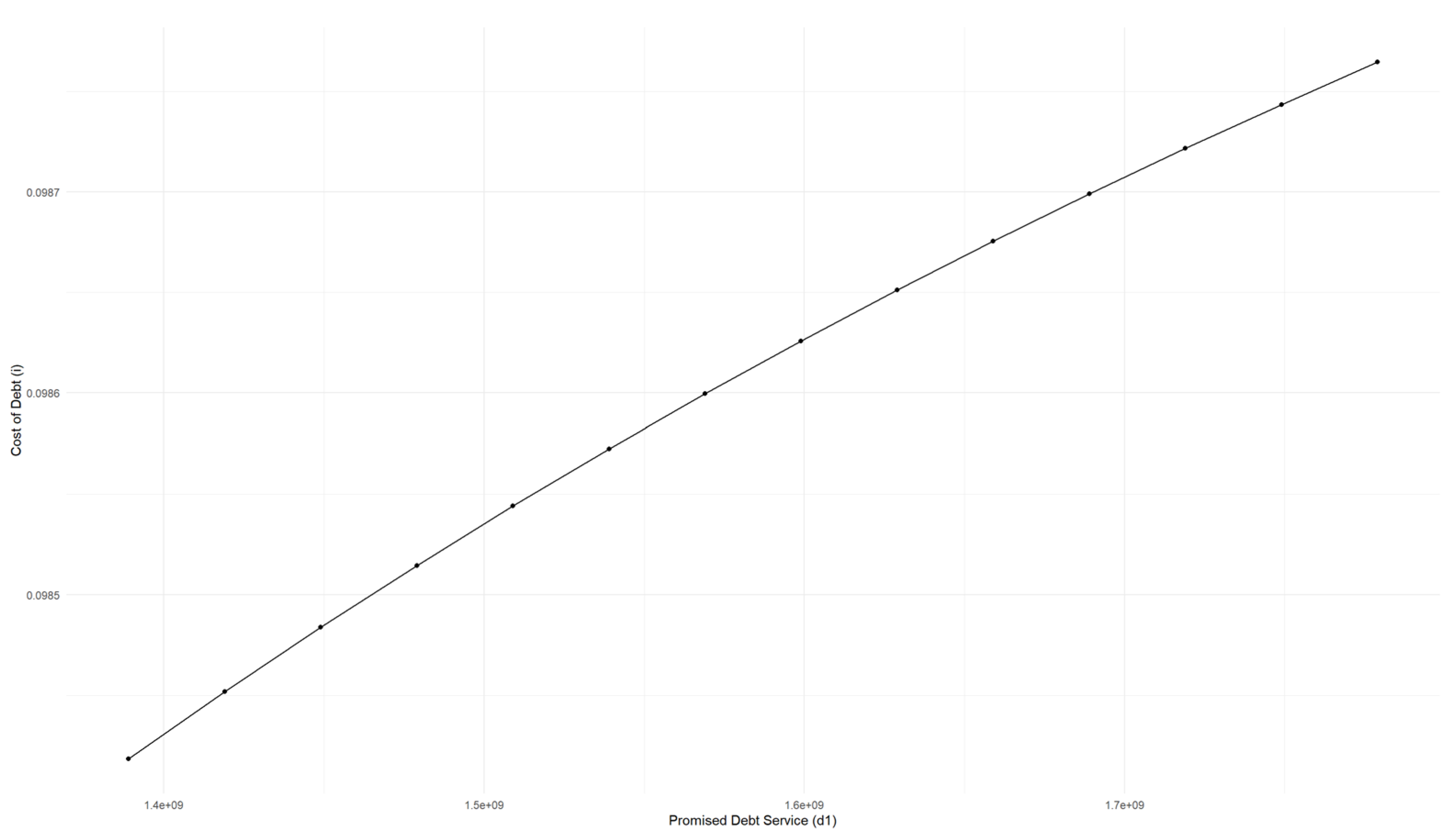
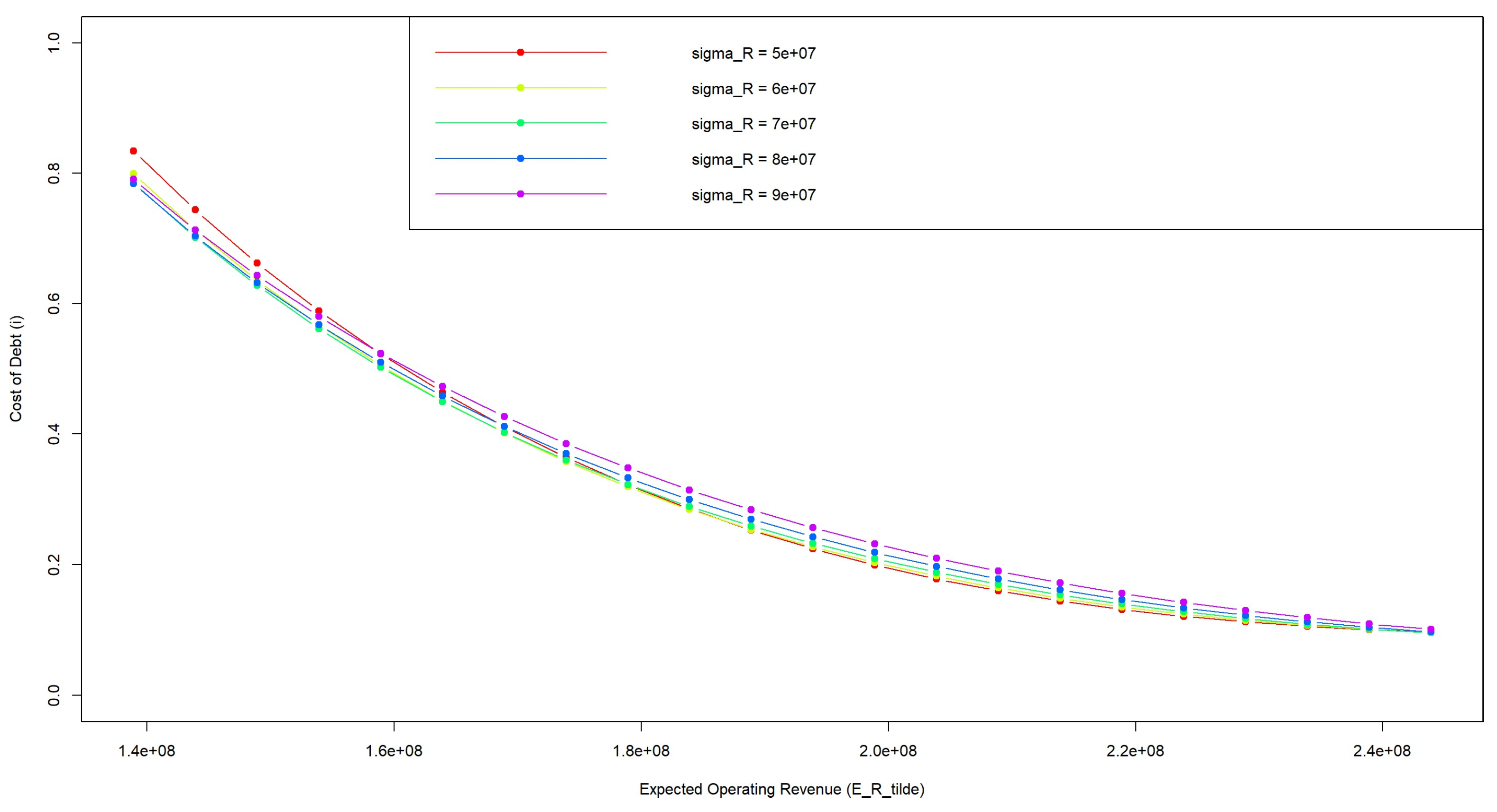
I perform a short sensitivity analysis to check the soundness of the model. First, I check the impact of increases in project leverage on the interest rate. Then, I check the impact of changes in operating revenues on the interest rate. Figure 3 shows that the interest rate increases as the d₁ increases, reflecting how increases in project leverage increases credit risk and therefore the cost of debt. Figure 4 shows that increases in the mean value of revenues E($\widetilde{{\displaystyle R}}$) lead to decreases in interest rate, while increases in the standard deviation of revenues σ_R lead to an overall increase in interest rate.

4.2. Climate-Informed Estimation of Loan Pricing

As recently as October 2023, Costa Rica, especially the region of San Jose, was hit by severe flooding causing major damage to roads and bridges. This led to 3000 people being temporarily housed in shelters.3

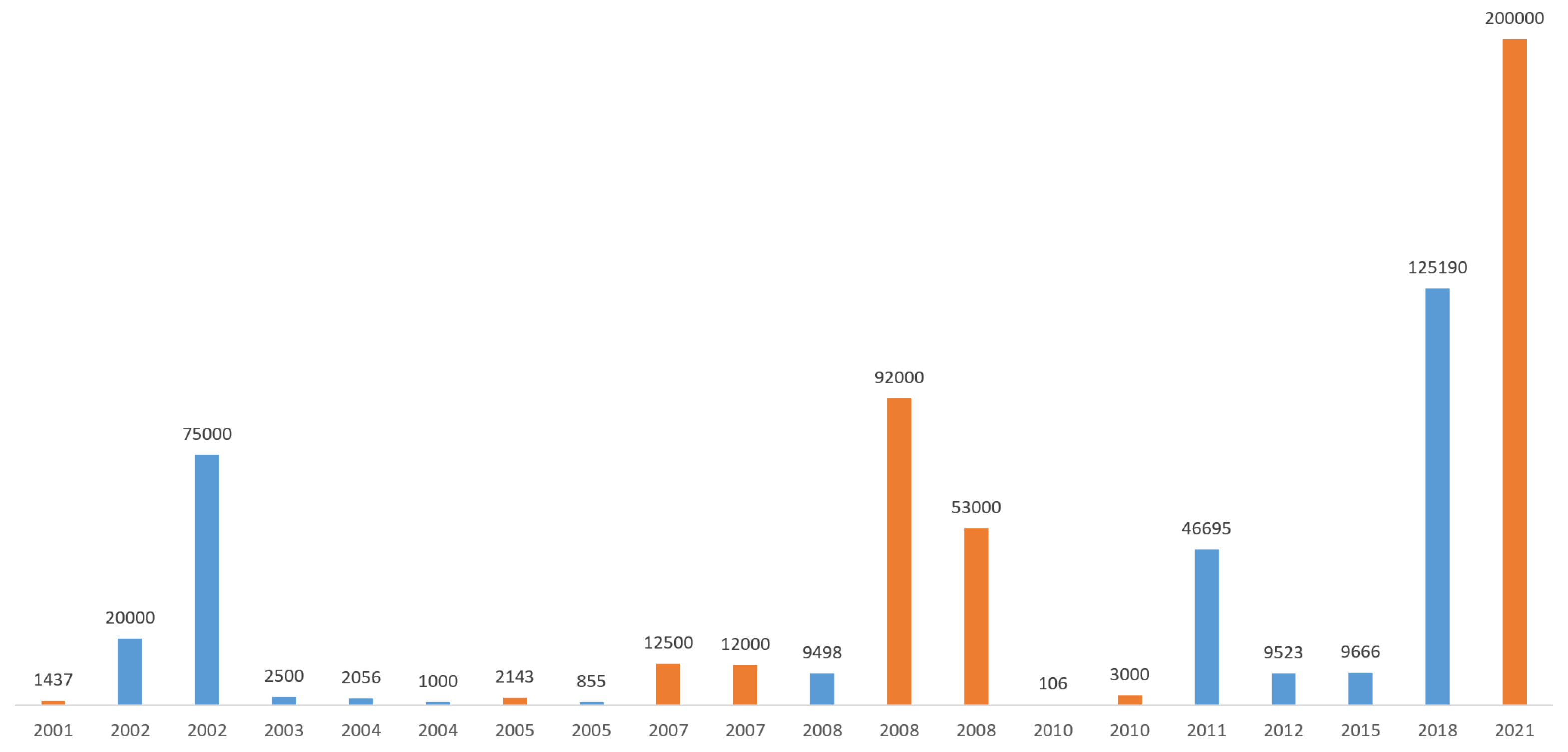
I use the AquaductFloods flood risk analysis tool to understand the GAM LRTs exposure to flood risk.4 Urban damage from flooding in Costa Rica is expected to increase from an annual average of USD 30.7 million in 2010 to USD 88 million in 2030, then to USD 147 million in 2050, and ultimately to USD 370 million in 2080 (Ward et al. 2020). Quesada-Román et al. (2021) analyzed 5987 hydrometeorological events in the GAM between 1970 and 2018 and found that 63.7% were floods. In another study, Quesada-Román (2022) created a flood risk index for 82 Costa Rican municipalities based on hazard, exposure and vulnerability. San Jose, the municipality where the GAM LRT project is happening, is ranked 12 out 82 municipalities in terms of flood risk. San Jose experienced 424 flood events that affected 4016 people (Quesada-Román 2022). The EM-DAT5 global extreme events database references 20 major flood events in Costa Rica between 2000 and 2023, of which 9 occurred in the San Jose area. Figure 5 shows in orange the floods that took place in San Jose.6

The GAM LRT technical documentation acknowledges the potential impact of flood on the infrastructure and includes an investment of USD 4.2 million in transverse and longitudinal drainage (IDOM CONSULTING 2020). However, this level of flood protection might not be sufficient in the future in the case of a pessimistic climate change scenario that would lead to an increase in the frequency and severity of floods in San Jose. The WRI Aqueduct estimates the current flood risk management in urban areas in Costa Rica to be fit for protection against a flood with an 18-year return period. It also estimates that in 2030, the measures will need to be adapted to protect against floods of higher severity with at least a 20-year return period. By 2080, these measures will need to be adapted to floods with a 61-year return period.

In the rest of this section, I estimate the premium associated with flood risk using the model presented in Section 3 on theoretical foundation.

4.2.1. Change in Average Revenues and Standard Deviation

I factor in flood risk considerations by altering the specifications of the normal distribution modelling the project revenues. I take the simplifying yet conservative assumption that change in the operating revenue’s mean and standard deviation is similar to changes in precipitations. The decrease in average precipitation and standard deviation will not translate into the same decrease for revenues, as revenues are not linearly proportional to precipitation. However, assuming such a linear relationship provides us with a worst-case scenario for the impact of precipitation trends on revenues.

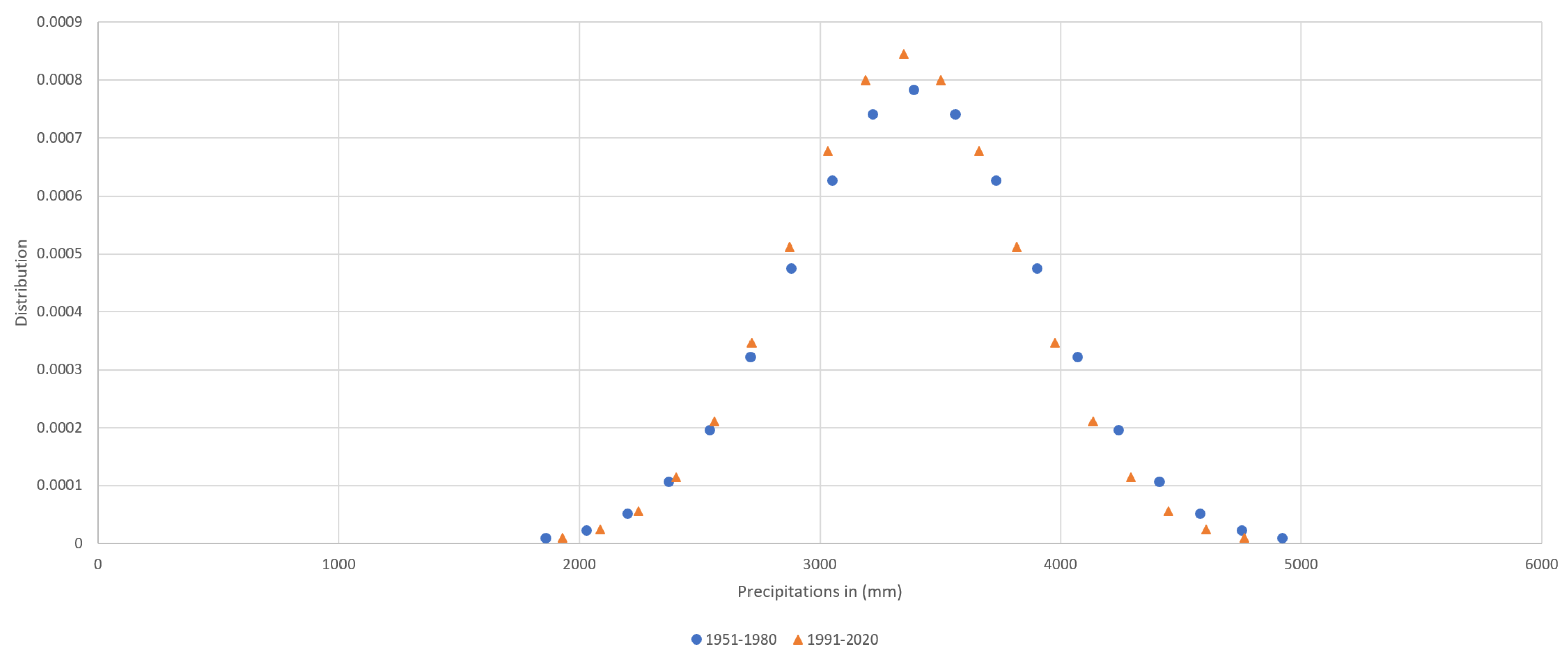
I use the World Bank’s precipitation variability and change in variability data to identify the change in average precipitation and standard deviation of precipitation between the period of 1951–1980 and 1991–2020—Figure 6. I find that the average value of precipitation decreased in the periods of 1951–1980 and 1991–2020 by 1.4%, while the standard deviation of precipitation also decreased by 7.5%.

I assume that project mean revenue E($\widetilde{{\displaystyle R}}$) also decreases by 1.4% from USD 247 million to USD 243.5 million, and project standard deviation of revenues decreases by 7.5% from USD 75 million to USD 69.4 million. The interest rate on the 10-year loan increases from the baseline value of 9.2% to 10% when including flood risk. There is an additional 80 basis points premium associated with flood risks corresponding to an additional USD 1.1 million in interest payments for the project.

4.2.2. Revenue Damage as a Pareto Distribution

In this section, I aim to estimate the interest rate based on expressing revenues following Equation (29) where the damage D to revenue follows a Pareto distribution.

$$\widetilde{{\displaystyle R}}=\stackrel{~}{{\displaystyle R_{\mathrm{base}}}}\times (1-D)$$

(29)

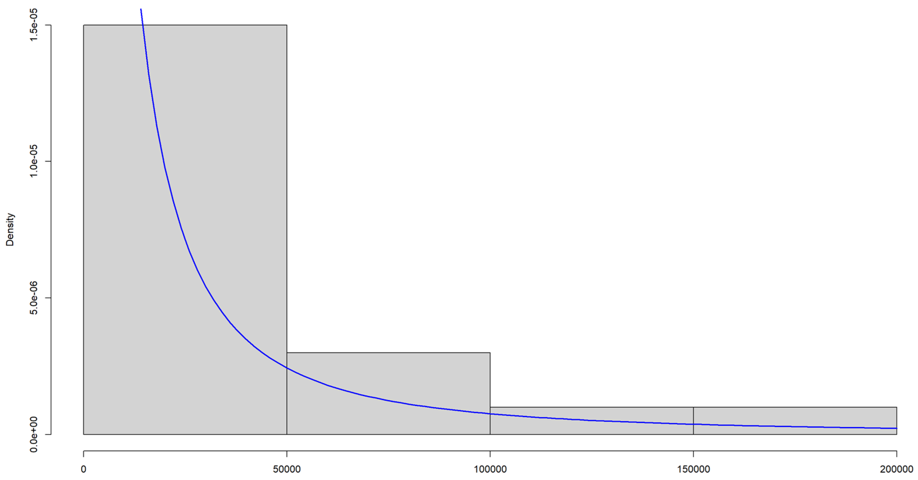
Ideally, I should fit a Pareto distribution to damage with LRT revenues. However, to the best of my knowledge, such data is not available. As an alternative, I fit a Pareto distribution to the flood damage data for Costa Rica referenced in the EM-DAT database and expressed it in terms of population affected. Figure 7 shows both the damage data and the fitted distribution. I estimate the scale parameter of the distribution x_m to be 6542 and the shape parameter α to be 0.84. I then re-calculate the interest rate i using the expression in Equation (17) for revenues and find the new interest rate to be close to 9.22% resulting in a flood risk premium of 2.63 basis points.

My results are based on historical values of damage. This method allows one to study the effect of future climate change either by increasing the scale parameter of the distribution or decreasing the shape parameter α in order to make the tails of the distribution heavier and reflect an increase in the severity. To illustrate this, I set two values for the shape parameter each representing a climate scenario in addition to the baseline value of 0.84.

Table 2. Interest rates corresponding to different shape values.

Shape Value	Interest Rate
Baseline	0.09227529
Mild (1.5)	0.09304102
Moderate (1.3)	0.09954218
Severe (1.1)	0.14977595

shows the different values of interest rates based on the value of α. As the shape parameter decreases, the interest rate increases. I notice a step change in the severe climate change scenario where the interest rate increases by more than 6% in comparison with the baseline scenario. This is an interesting value as it represents 3.7 times the cost of the project’s drainage infrastructure and potentially constitutes a compelling argument for adaptation investment. Studying the effect of climate change based on values of x_m and α estimated based on climate models could be a valuable research area to follow up on this paper.

4.2.3. Revenue Damage as a Poisson Distribution

It is also possible to model the damage to revenues as a Poisson distribution, as expressed in Equation (23). The Poisson distribution allows one to model the frequency of the flood events but not their severity. This distribution is easier to use in the case of the LRT project based on the available data. We know when the flood events happened, but we do not know each flood event’s damage in terms of interruptions to LRT traffic.

I fit a Poisson distribution to the annual occurrences of the flood events in Figure 6 and find a value of λ, the rate parameter in the Poisson distribution of 0.95. I assume the value of the damage in case of flooding, expressed as Severity in Equation (23), of 0.0704%. This value is the expected annual urban damage from riverine flooding in Costa Rica by 2030 based on Aqueduct floods—coastal flooding is not relevant since San Jose is located far from the coast (Ward et al. 2020).

In order to model the impact of flood events on revenues, I need to generate random flood events following the Poisson distribution. This means that every randomly generated set of flood events will result in a different interest rate. I therefore use simple simulation techniques to determine an expected value of the interest rate that I can then compare with the baseline interest rate.

I generate 1000 values of i using randomly generated numbers of flood events following a Poisson distribution of rate λ. I find that the expected value of i is 9.31% with a standard deviation of 0.07%. Using this approach, I estimate that the premium related to flood risk is 11.5 basis points.

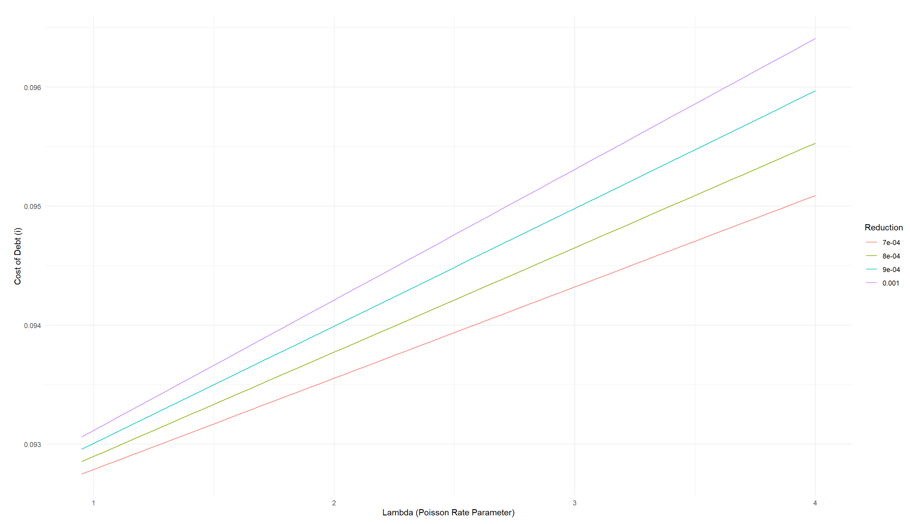
It is possible here to study the impact of future climate change through changing the value of λ. Figure 8 shows i as a function of the rate parameter λ of the Poisson distribution for different values of the damage or Severity. This distribution is the simplest to fit and study since data on future projects of frequency of flood events and damage are more readily available.

4.2.4. Incorporating Flood Risk in Project Costs

The Poisson distribution fitted previously can also be used to integrate flood risk consideration through the cost component of the project $\widetilde{{\displaystyle C}}$ as described in Equation (30).

c_v = c_vbase × (1 + Poisson(λ) × ExposureFactor × E(ClimateDamage))

(30)

I add a new component to the variable cost of the project c_v, equal to the damage multiplied by the Poisson distribution. I assume that the damage to the project, physical damage, is also equal to 0.0704% based on WRI Aquaduct. Using the rate parameter λ previously estimated, I generate 1000 values for the number of flood events and perform a simple simulation that shows that the average value of interest rate i is close to the baseline at 9.22% with a standard deviation of 2 basis points. Using this approach to pricing flood risk, I find that there is a 2.17 basis point premium to flood risk.

4.3. The Role of Adaptation Investment

In this section, I re-estimate the interest rate i focusing on the role of adaptation. The absence of a function linking adaptation investment to reduction in risk is a major gap in the climate finance literature. The results in this section are therefore illustrative. My main contribution is the closed form formulation of the function linking damage and adaptation investment.

I consider that the cost of the flood drainage infrastructure of USD 4.2 million is a fixed cost for adaptation. Then I integrate the incremental adaptation needs potentially resulting from the increase in flood risk due to climate change following Equations (31)–(33).

c_v = c_vbase × (1 + Poisson(λ) × AdaptFactor × E(ClimateDamage))

(31)

c_f = c_f base + AdaptInvestment

(32)

$$\mathit{AdaptFactor}=\frac{1}{1+\delta \times \mathrm{e}\mathrm{x}\mathrm{p}\left(\gamma \mathrm{A}\mathrm{d}\mathrm{a}\mathrm{p}\mathrm{t}\mathrm{I}\mathrm{n}\mathrm{v}\mathrm{e}\mathrm{s}\mathrm{t}\mathrm{m}\mathrm{e}\mathrm{n}\mathrm{t}\right)}$$

(33)

In absence of adaptation functions, I propose the logistic function framework and choose arbitrary values of δ (0.0002) and γ (0.0001). I estimate a new value of the interest rate i equal to 9.98%, or a 78 basis point premium associated to flood risk.

The parameter δ of our adaptation curve has an important economic significance. Figure 9 shows ExposureFactor as a function of AdpatInvestment for different values of δ while γ is fixed. The higher the value of delta, the smaller the cost to achieve a given level of reduction in exposure through reducing the exposure factor (δ). In simpler terms, δ represents how efficiently an adaptation investment reduces flood risk exposure; a higher δ means more bang for your buck in adaptation efforts. Therefore, δ informs about the effectiveness of a given investment in generation of adaptation to flood risk. Similarly, gamma (γ) measures the sensitivity of exposure reduction to changes in investment, with a focus on how small increases in adaptation spending can lead to significant decreases in risk exposure.

4.4. Concluding Discussion

The study finds that flood risk increases loan spreads for infrastructure projects by 2.6 to 78 basis points. This range is instructive when compared to related findings across different financing contexts. For instance, Painter (2020) observed a 23.4 basis point increase in municipal borrowing costs due to flooding, while Goldsmith-Pinkham et al. (2023) reported a 5.3 basis point rise in municipal bond yields from sea-level rise exposure. In the corporate sector, exposure to sea-level rise is linked to a 7 basis point premium on bonds (Allman 2022). Meanwhile, Kling et al. (2021) identified a broader impact of climate risk, increasing sovereign borrowing costs by an average of 0.66 percent over a period. These comparisons highlight the varied but consistently negative impact of flood and climate risks on financing costs across sectors, with our findings sitting within the observed range for infrastructure financing specifically.

The theoretical foundation, based on the CAPM-derived expression of interest rates, offers an avenue of pricing climate risk to lenders and investors in infrastructure projects. We have seen however, as summarized in

Table 3. Comparison of pricing approaches and flood risk premiums.

Pricing Approach	Average Cost of Debt	i Flood Risk Premium in bps
Baseline	0.0920
Pareto distribution	0.0922	2.63
Revenues, Poisson distribution	0.0931	11.52
Cost, Poisson distribution	0.0922	2.17
Cost, Poisson with adaptation	0.098	78

, that choices of how to use the theoretical foundation results in different estimations of the flood risk premium. When climate risk is reflected through revenues, the choice of probability distribution for climate hazards leads to significant changes in climate risk premium. The premium also changes if climate risk is reflected through costs rather than revenues. Further incorporating adaptation considerations also leads to a different outcome in terms of premium. It is therefore important to identify principles for the application of this theoretical foundation.

The first question when applying the theoretical foundation is whether to factor in climate risks through revenues, costs, or both. Infrastructure projects can include financial risk management mechanisms that can reduce the financial impact of climate risks as they guarantee revenues or insure against losses.

A factor to consider when selecting the climate pricing model is the revenue model of the infrastructure. If a guaranteed revenue mechanisms is in place, such as a Power Purchase Agreement (PPA) for electricity generation infrastructure, the revenues might not be affected by climate hazard. For infrastructure projects with availability-based revenue models, such metro projects, where a portion of a project’s revenues is guaranteed, the impact of climate hazard will depend on the service agreement and the minimum service thresholds. The pricing of climate risk through revenues is relevant. For infrastructure projects with market-based revenue models, or no guaranteed revenues, such as airports or toll roads, climate risk pricing through revenues is relevant.

The second type of risk management mechanisms that can influence the choice of climate pricing model is related to costs. If the existing insurance and risk transfer mechanisms already cover damages relative to climate hazard, it might not be necessary to also reflect it in the pricing. In such a case, it is important to evaluate the insurance policy to ensure that the coverage includes appropriate climate event frequency and magnitude.

Data availability and our understanding of the nature of the climate hazards are other factors determining the choice of the approach. For instance, if a climate risk analysis reveals that the project is more exposed to chronic climate hazards, pricing approaches relying on updated means and variance of revenues are more appropriate. If the infrastructure is exposed to acute climate hazard, i.e., extreme events, it is more appropriate to use the Pareto and Poisson-based approaches that better capture extremes.

An assessment of data availability and the quality of climate modelling is a pre-requisite to choosing between a Pareto and Poisson distribution. When accurate damage functions for a given hazard are available, it is possible to successfully use a Pareto distribution, as both the frequency of the climate hazard and the subsequent impacts are necessary to fit the distribution. In the case of the GAM LRT project in this paper, I resorted to using flood damage at country-level to fit the Pareto distribution in absence of a flood depth– damage function. When such information on damage is lacking, it could be more appropriate to adopt a Poisson distribution that only requires the event occurrence to be fitted.

Another critical data-related factor to consider is the availability of historical data on revenues and costs. This data is often not available for greenfield infrastructure projects. In such a case, a baseline needs to be determined based on the financial data of another project of similar characteristics, including climate risk exposure and vulnerability.

The framework outlined in this paper illustrates the inherent complexities of embedding physical climate risk into financial practices as described in

Table 4. Key challenges to implementation of the approach.

Modeling Step	Challenges
Baseline estimation of loan pricing	- Estimating financial variables such as the risk-free rate and market return.
	- Adopting revenue scenarios without considering the full range of potential climate impacts.
Climate-informed estimation of loan pricing	- Assessing the project’s exposure to flood risk using historical data and future projections.
	- Balancing the simplification in modeling approaches with the need for accurate risk assessment.
Adjustments for revenue changes	- Making conservative assumptions about the relationship between precipitation changes and revenue impacts.
	- Reliance on external data sources for precipitation variability, adding another layer of uncertainty.
Modeling revenue damage	- Choosing the appropriate distribution for modeling flood damage, each with its limitations in representing the complexity of climate impacts.
	- The absence of specific damage data necessitates assumptions that may oversimplify the actual risk.
Incorporating flood risk in costs	- Integrating flood risk into project costs requires simulations that may not fully capture the potential range of flood impacts.
	- The challenge of quantifying the variable cost component related to flood damage.
Role of adaptation investment	- The difficulty in quantifying the effectiveness of adaptation measures without established methodologies.
	- Making arbitrary choices for modeling parameters due to the lack of detailed guidance on linking adaptation investments to risk reduction.

. Diverging from the array of approaches seen in the UNEP FI7 exercise described in

Table 5. UNEP FI pilot climate risk assessment—assessment characteristics.

Scenario	Hazards	Methodology
RCP 4.5/SSP2–4.5	Sea level rise, flooding, temperature extremes, etc.	World Sustainability’s adjusted risk scale, high risk identification, and bespoke engagement details.
RCP 8.5/SSP5–8.5	Sea level rise, flooding, temperature extremes, etc.	Altitude’s sector-geography risk analysis using IPCC, TCFD, EU Taxonomy standards.
RCP 4.5/SSP2–4.5	Eight climate hazards within CLIMATIG for year 2050.	CLIMATIG Score averaging individual hazard scores per asset.
RCP 4.5/SSP2–4.5	Flood, cyclone, etc. with specific spatial resolutions.	EY CAP’s indicator-based scoring system, considering multiple climate model outputs.
RCP 4.5/SSP2–4.5	Sea level rise, scored hazards.	Munich Re’s proprietary models with sector-specific vulnerability factors.
RCP 4.5/SSP2–4.5	Hazards covered by Climate Excellence excluding water stress.	Estimation of expected losses with a scoring system reflecting the asset value impact.
RCP 4.5/SSP2–4.5	Hazards aligned with non-parametric probability distributions.	Riskthinking.AI’s stochastic, algorithmic approach using the Dembo Method for risk scoring.

, it advances the analysis by factoring in the costs and benefits of adaptation measures and offers a detailed, site-specific assessment that enhances the precision over standard portfolio analyses. Employing forward-looking scenarios, the framework utilizes distinct climate projections, integrating these into a pricing model. It also involves a discerning process of parameter selection, reflecting a strategic approach to assumptions that might contrast with the broader methodologies used in UNEP FI assessments.

5. Limitations of the Study

The application of the Capital Asset Pricing Model (CAPM) to price climate risks in infrastructure loans, while innovative, encounters several limitations. CAPM’s reliance on beta as a sole measure of risk overlooks the complex and multifaceted nature of climate risks, which can impact infrastructure projects in diverse ways beyond general market fluctuations. The model’s foundational assumptions—such as the existence of a homogeneous market portfolio and a risk-free rate—are problematic in the context of climate change, which introduces specific, tangible risks not captured by abstract market portfolios or the notion of risk-free investments.

Moreover, CAPM presupposes investor rationality and homogeneity in risk perception, failing to account for the varied and dynamic nature of climate risks and investors’ responses to them. This oversight highlights the need for a more nuanced approach that incorporates specific climate risk assessments and adaptation considerations into traditional financial models.

Acknowledging these limitations is crucial in refining the framework outlined in this study, underscoring the importance of complementing CAPM with detailed climate risk analyses to achieve a more accurate and comprehensive pricing model for infrastructure loans.

Another one of the key gaps identified during this study is the absence of data on the sensitivity of infrastructure projects’ revenues and costs to climate hazards. This limitation restricts the depth of analysis possible regarding the financial impact of climate risks on infrastructure financing. Another gap is the absence of functions linking adaptation investment to reduction in exposure to hazards. The development of such functions is crucial for financial institutions to accurately price the exposure and vulnerability to climate risks and to incentivize adaptation investment.

6. Prospects for Further Research

The theoretical foundation outlined in this paper offers several avenues for enhancement and further exploration. For instance, the foundation can be enriched to include the pricing of multiple climate hazards, acknowledging that an infrastructure project is likely exposed to various climate risks. The interaction and accumulation of these risks could significantly affect project financing and risk management strategies. Additionally, there is potential to expand the model to assess climate risk for portfolios of infrastructure projects. This expansion would enable financial decision-makers to evaluate the benefits of sector and geographic diversification more comprehensively, potentially uncovering strategies to mitigate climate risk across different investments.

References

- Allman, Elsa. 2022. Pricing climate change risk in corporate bonds. Journal of Asset Management 23: 596–618. [Google Scholar] [CrossRef]
- Assab, Abderrahim. 2023a. Did We Open The Floodgates? Flood Damage and Infrastructure Loan Defaults. [Google Scholar]
- Assab, Abderrahim. 2023b. Flood Insurance, Building Codes, and Public Adaptation: Implications for Airport Investment and Financial Constraints. Journal of Risk and Financial Management 16: 363. [Google Scholar] [CrossRef]
- Bolton, Patrick, Morgan Després, Luiz Awazu Pereira da Silva, Frédéric Samama, and Romain Svartzman. 2020. The green swan. In BIS Books. Basel: BIS. [Google Scholar]
- Campiglio, Emanuele, Louis Daumas, Pierre Monnin, and Adrian von Jagow. 2023. Climate-related risks in financial assets. Journal of Economic Surveys 37: 950–92. [Google Scholar] [CrossRef]
- Carlin, David, Josefine Falk, Drew Johnson, Wenmin Li, and Lea Lorkowski. 2023. The 2023 Climate Risk Landscape. Policy Common. [Google Scholar]
- Dias, Antonio, Jr., and Photios G. Ioannou. 1995. Debt capacity and optimal capital structure for pri- vately financed infrastructure projects. Journal of Construction Engineering and Management 121: 404–14. [Google Scholar]
- Dodman, David Satterthwaite vid. 2009. The costs of adapting infrastructure to climate change. Assessing the Costs of Adaptation to Climate Change: A Review of the UNFCCC and Other Recent Estimates 73. [Google Scholar]
- Fama, Eugene F., and Kenneth R. French. 1996. The CAPM is wanted, dead or alive. The Journal of Finance 51: 1947–58. [Google Scholar]
- Fankhauser, Samuel. 2010. The costs of adaptation. Wiley Interdisciplinary Reviews: Climate Change 1: 23–30. [Google Scholar] [CrossRef]
- Giglio, Stefano, Bryan Kelly, and Johannes Stroebel. 2021. Climate finance. Annual Review of Financial Economics 13: 15–36. [Google Scholar] [CrossRef]
- Goldsmith-Pinkham, Paul, Matthew T. Gustafson, Ryan C. Lewis, and Michael Schwert. 2023. Sea-level rise exposure and municipal bond yields. The Review of Financial Studies 36: 4588–635. [Google Scholar] [CrossRef]
- Gupta, Amrita, Caleb Robinson, and Bistra Dilkina. 2018. Infrastructure resilience for climate adaptation. Paper presented at the 1st ACM SIGCAS Conference on Computing and Sustainable Societies, San Jose, CA, USA, June 22–28; pp. 1–8. [Google Scholar]
- Hong, Harrison, Neng Wang, and Jinqiang Yang. 2023. Mitigating disaster risks in the age of climate change. Econometrica 91: 1763–802. [Google Scholar] [CrossRef]
- Hughes, Gordon, Paul Chinowsky, and Ken Strzepek. 2010. The costs of adaptation to climate change for water infrastructure in OECD countries. Utilities Policy 18: 142–53. [Google Scholar] [CrossRef]
- IDOM CONSULTING. 2020. Studies for the Technical, Economic-Financial, Environmental, Vul-nerability & Social Feasibility for the Construction, Equipment, Test & Commissioning, Operation and Maintenance under Works Concession with Public Service of the Passenger Rapid Train in the Great Metropolitan Area: Fourth Report: Economic and Financial Survey. Technical Report. Bilbao: IDOM CONSULT ING. [Google Scholar]
- In, Soh Young, Berk Manav, Clothilde Venereau, Luis Enrique Cruz Rodriguez, and John Weyant. 2021. Pricing Climate Risks of Energy Investments: A Comparative Case Study. Available online: https://papers.ssrn.com/sol3/papers.cfm?abstract_id=3779228 (accessed on 20 January 2024).
- Jagannathan, Ravi, and Ellen R. McGrattan. 1995. The CAPM debate. Federal Reserve Bank of Minneapolis Quarterly Review 19: 2–17. [Google Scholar]
- Karydas, Christos, and Anastasios Xepapadeas. 2022. Climate change financial risks: Implications for asset pricing and interest rates. Journal of Financial Stability 63: 101061. [Google Scholar] [CrossRef]
- Kelly, David L., and Renato Molina. 2023. Adaptation Infrastructure and its Effects on Property Values in the Face of Climate Risk. Journal of the Association of Environmental and Resource Economists 10: 1405–38. [Google Scholar] [CrossRef]
- Kim, E. Han. 1978. A mean-variance theory of optimal capital structure and corporate debt capacity. The Journal of Finance 33: 45–63. [Google Scholar]
- Kim, Kyeongseok, Sooji Ha, and Hyoungkwan Kim. 2017. Using real options for urban infrastructure adaptation under climate change. Journal of Cleaner Production 143: 40–50. [Google Scholar] [CrossRef]
- Kling, Gerhard, Ulrich Volz, Victor Murinde, and Sibel Ayas. 2021. The impact of climate vulnerability on firms’ cost of capital and access to finance. World Development 137: 105131. [Google Scholar] [CrossRef]
- Levy, Haim. 2010. The CAPM is alive and well: A review and synthesis. European Financial Management 16: 43–71. [Google Scholar] [CrossRef]
- Luo, Tianyi, Yan Cheng, James Falzon, Julian Kölbel, Lihuan Zhou, Yili Wu, and Amir Habchi. 2023. A framework to assess multi-hazard physical climate risk for power generation projects from publicly-accessible sources. Communications Earth & Environment 4: 117. [Google Scholar]
- Narain, Urvashi, Sergio Margulis, and Timothy Essam. 2016. Estimating costs of adaptation to climate change. In International Climate Finance. London: Routledge, pp. 90–113. [Google Scholar]
- Painter, Marcus. 2020. An inconvenient cost: The effects of climate change on municipal bonds. Journal of Financial Economics 135: 468–82. [Google Scholar] [CrossRef]
- Quesada-Román, Adolfo. 2022. Flood risk index development at the municipal level in Costa Rica: A methodological framework. Environmental Science & Policy 133: 98–106. [Google Scholar]
- Quesada-Román, Adolfo, Ernesto Villalobos-Portilla, and Daniela Campos-Durán. 2021. Hydrometeoro- logical disasters in urban areas of Costa Rica, Central America. Environmental Hazards 20: 264–78. [Google Scholar] [CrossRef]
- Sarmento, Joaquim Miranda, and Miguel Oliveira. 2018. Use and limits in project finance of the capital asset pricing model: Overview of highway projects. European Journal of Transport and Infrastructure Research 18. [Google Scholar] [CrossRef]
- Savoia, Jos’e Roberto Ferreira, José Roberto Securato, Daniel Reed Bergmann, and Fabiana Lopes da Silva. 2019. Comparing results of the implied cost of capital and capital asset pricing models for infrastructure firms in Brazil. Utilities Policy 56: 149–58. [Google Scholar] [CrossRef]
- Stewart, Mark G., and Xiaoli Deng. 2015. Climate impact risks and climate adaptation engineering for built infrastructure. ASCE-ASME Journal of Risk and Uncertainty in Engineering Systems, Part A: Civil Engineering 1: 04014001. [Google Scholar] [CrossRef]
- Ward, Philip J., Hessel C. Winsemius, Samantha Kuzma, Marc F. P. Bierkens, Arno Bouwman, Hans De Moel, Andrés Díaz Loaiza, Dirk Eilander, Johanna Englhardt, Gilles Erkens, and et al. 2020. Aqueduct Floods Methodology. Washington, DC: World Resources Institute, pp. 1–28. [Google Scholar]
- Wibowo, Andreas. 2006. CAPM-based valuation of financial government supports to infeasible and risky private infrastructure projects. Journal of Construction Engineering and Management 132: 239–48. [Google Scholar] [CrossRef]
Figure 1.
Relationship between adaptation investment and exposure factors for different values of δ and γ.
Figure 2.
GAM LRT revenues under baseline scenario.
Figure 3.
Interest rate on debt as a function of leverage.
Figure 4.
Interest rate vs revenue for different revenue standard deviations.
Figure 5.
EM-DAT flood event and affected population in Costa Rica between 2000 and 2021.
Figure 6.
Precipitation variability and change in variability in Costa Rica—World Bank Climate Change Knowledge Portal.
Figure 7.
Flood-affected population and fitted Pareto distribution.
Figure 8.
Cost of debt as a function of λ for different urban damage values.
Figure 9.
Adaptation effectiveness of different values of δ.