A New Proxy for Estimating the Roughness of Volatility

Abstract

In this paper, we propose a new proxy for the unobserved volatility process that will allow us to better understand and hence model a rough or persistent volatility. Starting with a stochastic volatility model with minimal assumptions on the volatility process, we calibrate the model to options’ data and their sensitivities to obtain an implied volatility process. Starting with this new proxy, we then study the roughness/persistence of the volatility using S&P 500 European put option daily data. We then estimate the Hurst index, i.e., roughness/smoothness parameter, of the volatility with various techniques to find that the volatility does exhibit a rough behavior, even in a low-frequency framework.

1. Introduction

The modeling of stochastic volatility in continuous time traditionally falls in the semi-martingale domain, where the dynamics of the stock follow a diffusion driven by a Brownian motion and the dynamics of the volatility are described by a mean-reverting stochastic differential equation driven by another Brownian motion. Since the introduction of stochastic volatility models (Cox et al. 1985; Garman 1976; Hull and White 1987), practitioners have been able to better understand stylized facts that emerge in derivative pricing, such as the volatility clustering or the skewness of volatility smiles (Fouque et al. 2000), e.g., Ait-Sahalia et al. (2001), Avallaneda et al. (1997), Szczygielski and Chipeta (2023), Aggarwal et al. (1999), Coleman et al. (1999), Dumas et al. (1997), Gatheral (2006).

However, there are still certain aspects of the volatility that cannot be captured by these more traditional models. For example, the momentum observed in the conditional variance as well as the high correlation of past lags of the volatility with the present, the so-called volatility persistence, have been documented in the literature by Andersen and Bollerslev (1997) and Breidt et al. (1998). Specifically, Andersen and Bollerslev (1997) and Andersen et al. (2001) analyzed the autocorrelation of the returns of Deutschemark–U.S. dollar, Yen–U.S. dollar foreign exchange rates as well as the returns of the S&P 500 index using high-frequency intraday data to discover a slow persistence in the decay rate, while Breidt et al. (1998) focused on several market indexes’ daily returns to also discover a slow decay in the autocorrelation structure. Even before these studies, the presence of long-range dependence in the volatility has been observed in Ding et al. (1993), where the authors analyzed the autocorrelation structure of the S&P 500 returns.

In order to better describe volatility persistence, Comte and Renault (1998) introduced the long-memory stochastic volatility model (LMSV), according to which the stock follows the same diffusion as in the traditional framework, while the volatility is described by a stochastic differential equation driven by a fractional Brownian motion with $H>1/2$, a process that captures persistence (for the mathematical definition, refer to Section 1.1). Since then, significant progress has been made regarding LMSV models. Comte et al. (2012) proposed a long-memory Heston model for which they introduced related simulation methods and Alos and Yang (2017) introduced a pricing method and an implied volatility formula for a fractional Heston model. The implied volatility term structure has also been studied by Garnier and Sølna (2017) and lattice-based pricing algorithms as well as calibration methods have been proposed in Chronopoulou and Viens (2012).

From a different point of view, the trajectories of the volatility estimated using high-frequency data are not as smooth as those of a fractional Brownian motion with $H>1/2$. In order to explain this rough behavior of the volatility process, Gatheral et al. (2018) introduced a rough volatility model, according to which the log-volatility behaves similarly to a fractional Brownian motion with $H<1/2$. In this context, Gatheral et al. (2018) and Fukasawa et al. (2019) analyzed ultra-high-frequency data of DAX and Bund future contracts, and high-frequency data from S&P and NASDAQ indices. Also, Da Fonseca and Zhang (2019) conducted an analysis on the realized variance of VIX, using 5 min high-frequency VIX data, with the result showing that volatility of volatility is also rough. Furthermore, a similar behavior is documented in Livieri et al. (2018) using high-frequency bid-ask data of options on S&P 500 via the Medvedev–Scaillet corrected implied volatility (Medvedev and Scaillet 2007).

Although more sophisticated volatility models better describe empirical stylized facts, the estimation of their parameters and their calibration to real data is a highly complicated task, due to the hidden nature of the volatility process. In the traditional framework, filtering methods have been introduced for such purposes (Kristensen 2010). However, similar statistical techniques for long-range dependent or rough models are still an active research area. Therefore, when it comes to financial applications, in order to assess the validity of these models, one needs to use calibration techniques in conjunction with the use of volatility proxies, i.e., observable quantities from the market that mimic the volatility behavior.

One common quantity that has been proven useful in high-frequency data is the integrated volatility, which is calculated via the quadratic variations of the log-returns, also called realized volatility (Barndorff-Nielsen and Shephard 2002). However, this proxy is subject to micro-structure effects and turns out to be a noisy approximation (Zhang et al. 2005; Zhou 1996). Other non-parametric, kernel-based techniques (Jacod 2019; Kristensen 2010; Xiu 2010) have also been proposed, but are in general unreliable due to the ad hoc choices of the hyper-parameters involved.

The realized volatility or the output of a non-parametric algorithm both limit approximations of the volatility process, and thus in order to be accurate in practice, they require high- or ultra-high-frequency observations. In a low-frequency setting, such approximations are neither reliable nor feasible; therefore, one has to resort to other methods. The most popular approach is to consider the implied volatility or a proxy of the implied volatility. A common proxy in this context is the VIX, which is the volatility index from the Chicago Board Options Exchange (CBOE) representing the market expectation of volatility in the future. This is also considered to be the implied volatility of a fictitious at-the-money option with 30-day maturity. However, there is empirical evidence (Aı et al. 2007; Chow et al. 2018) suggesting that the VIX tends to overestimate when volatility is low and underestimate when volatility is high, which implies that the resulted sample path is always smoother, making it unreliable in the study of rough volatility.

In this paper, our first contribution is the introduction of a new volatility proxy for the study of rough or persistent volatility that works well in a low-frequency framework. Specifically, instead of estimating the volatility via filtering algorithms, we use daily observations of cumulative option trading entries and their Greeks to calibrate a stochastic volatility model (with minimal assumptions on the volatility process) to the data by solving a quadratic optimization problem for a range of strike prices and maturities. The solution to this problem provides us with a proxy for the unobserved volatility process. This volatility value is in principle static (for a fixed time t), but when the algorithm is repeated for consecutive days, we can extract a time series of implied volatilities that approximates the true volatility process.

Starting with this new proxy, our second goal is to use various methods for estimating the persistence/roughness of the volatility process to better understand its behavior. Specifically, we use estimation techniques in the literature to study the robustness of the estimators of the Hurst index, which is the parameter that describes the “memory” of the volatility. When we apply our techniques to European put options on the S&P 500, we uncover a rough behavior of the volatility, i.e., $H<1/2$, even in a low-frequency setting. We also investigate empirically whether the Hurst parameter can be considered a constant and we observe that the Hurst index varies largely, suggesting that it is a local parameter that is not to be considered a constant in the long run.

The structure of the paper is as follows: In Section 1, we give a short introduction to the models considered along with the relevant mathematical background. In Section 2, we introduce the proposed methodology for the volatility estimation, and we discuss existing Hurst index estimation methods. In Section 3, we compute the implied volatility process using S&P 500 daily options data. We compare our method with the VIX index and we study changes in the roughness of the volatility over different time horizons. Finally, in Section 4, we conclude and discuss the implications of our results.

1.1. Mathematical Background and Assumptions

In this section, we introduce the underlying model for fractional volatility and we briefly discuss the necessary mathematical background. Throughout this paper, we assume that there exists a filtered probability space $(\Omega ,\mathcal{F},{\mathcal{F}}_t,P)$, and all the processes that follow are adapted to the given filtration.

The cornerstone of our model is the fractional Brownian motion (fBm), which can be thought of as an extension of a standard Brownian motion with dependent increments. Rigorously, a fractional Brownian motion $\{B_t^H;t\ge 0\}$ with $H\in (0,1)$ is a centered Gaussian process with covariance function given by

$$\mathbb{E}\left(B_t^H{B}_s^H\right)=\frac{1}{2}\left(t^{2H}+s^{2H}-{|t-s|}^{2H}\right)$$

and a.s. continuous sample paths Mandelbrot and Van Ness (1968).

The value of $H\in (0,1)$ (also called Hurst index) determines both pathwise and probabilistic properties of fBm. When $H=1/2$, we recover the standard Brownian motion. As in the classical case, for the fBm, the initial value $B_0^H=0\mathrm{a}.\mathrm{s}.$ and its increments are stationary, i.e., $B_t^H-B_s^H{=}_d{B}_{t-s}^H$. Unlike the standard Brownian motion, fBm has increments that exhibit long-range dependence (also called long memory or persistence) when $H>1/2$ and anti-persistence (or roughness) when $H<1/2$. The covariance of the increments of fBm, $B_{t+h}^H-B_t^H$ and $B_{s+h}^H-B_s^H$ with $t-s=nh$ can be computed as ${\rho }_n\left(h\right)=1/2h^{2H}\left[{(n+1)}^{2H}+{(n-1)}^{2H}-2n^{2H}\right]$. The sample paths of the fractional Brownian motion are almost surely Hölder continuous of order strictly less than H. Also, the fBm is self-similar, which means that the distribution of $B_{at}^H$ and the distribution of $a^{-H}{B}_t^H$ are the same for any $a>0$. For more details, we refer the reader to Mandelbrot and Van Ness (1968) and Beran et al. (2016).

The model we consider in this paper is a stochastic volatility model, in which the asset price at time t, denoted by $\{S_t;t\ge 0\}$, is described by

$$d{S}_t=r{S}_{t}dt+S_t{\sigma }_{t}d{B}_t$$

(1)

under the risk-neutral measure, where r is the risk-free rate, which we assume to be constant. This assumption can be relaxed and r can be locally constant or random. $\{B_t;t\ge 0\}$ is a Brownian motion and $\{{\sigma }_t;t\ge 0\}$ is the volatility process. For the volatility process $\{{\sigma }_t;t\ge 0\}$, we assume that the logarithm of the volatility, namely $Y_t=log\left({\sigma }_t\right)$, is an adapted square integrable stochastic process. We also assume that $\{Y_t;t\ge 0\}$ is a Gaussian process with stationary increments.

The fractional stochastic volatility model has an autocorrelation structure similar to that of fBm, and is described as follows: If we define the pth order variogram of $\left\{Y_t\right\}$, for any $p>0$, we have

$${\gamma }_p(h;Y)=\mathbb{E}\left[\right|Y_{t+h}-Y_t{|}^p]$$

Then, we assume that ${\gamma }_p(h;Y)$ satisfies the following properties:

(a)

For some $H\in (0,1)$, we have:

$${\gamma }_2(h;Y)=h^{2H}L\left(h\right)$$

with $L\left(h\right)$ continuously differentiable and bounded away from 0 in a neighborhood of $h=0$. $L\left(h\right)$ is also assumed to be slowly varying at 0, i.e.,

$$\underset{h\to 0}{lim}\frac{L\left(th\right)}{L\left(h\right)}=1\mathrm{for}\mathrm{any}t>0$$

(b)

$$\frac{d^2}{d{h}^2}{\gamma }_2(h;Y)=h^{2H-2}{L}_2\left(h\right)$$

where $L_2(·)$ is another slowly varying function,

(c)

There exists $b\in (0,1)$ with

$$\underset{x\to 0}{lim\; sup}\underset{h\in [x,x^b]}{sup}\left|{\displaystyle \frac{L_2\left(h\right)}{L\left(h\right)}}\right|<\infty$$

It is easy to check that if $\left\{Y_t\right\}$ is a fractional Brownian motion all the properties above will be satisfied. Thus, fractional Brownian motion is a special case of processes satisfying all the above and the processes satisfying all the above properties can be thought of as an extension to the fractional Brownian motion Beran et al. (2016).

2. Estimation of Implied Volatilities via Calibration

In this section, we develop a framework for estimating the unobserved volatility process using low-frequency option data. We also discuss the most popular methods in the literature to estimate the Hurst index of the volatility process.

2.1. A New Volatility Proxy

Assume that the asset follows the geometric Brownian motion defined in (1), in which the volatility ${\sigma }_t$ is an adapted stochastic process. At this stage, we do not need to further specify the dynamics of ${\sigma }_t$. Instead, following the approach in Carr and Wu (2016), for each vanilla option, we define the dynamics of the implied volatility to be:

$$d{I}_t(K,T)={\mu }_{t}dt+{\omega }_{t}d{Z}_t,$$

(2)

where K is the strike price of the option and T is the maturity time of the option. $\{{\mu }_t;t\ge 0\}$ and $\{{\omega }_t;t\ge 0\}$ are two adapted processes and $Z_t$ is another Brownian motion, correlated with $B_t$ in (1) with correlation ${\rho }_t$. The dynamics of $I_t$ are not dependent on K and T, but the initial value of $I_t$ is. Using the Black–Merton–Scholes pricing formula, the put option price, $P(t,K,T)$, can be expressed as

$$P(t,K,T)=BS(S_t,I_t,t),$$

where $BS(S_t,I_t,t)$ stands for the Black–Scholes formula, with arguments for the instant price $S_t$, the implied volatility $I_t$ and time t. Assume there is a basis call option at $(K_0,T_0)$ and no dynamic arbitrage is allowed on any put option at $(K,T)$ relative to the portfolio of basis option, stock and cash. Then, according to Proposition 1 (Carr and Wu 2016), after applying Itô’s formula to the risk-neutral portfolio of a put option at $(K,T)$, the basis call option at $(K_0,T_0)$, and the underlying stock, we have

$$-P_t+r-r{P}_S{S}_t={\mu }_t{P}_{\sigma }+\frac{1}{2}{\sigma }_t^2{S}_t^2{P}_{SS}+{\rho }_t{\omega }_t{\sigma }_t{S}_t{P}_{S\sigma }+\frac{1}{2}{\omega }_t^2{P}_{\sigma \sigma }$$

(3)

where the subscripts denote the corresponding derivatives of the option price P. Namely,

$$P_S:=\frac{\partial BS(S_t,I_t,t)}{\partial S_t}(\mathrm{the}\mathrm{Delta}),P_t:=\frac{\partial BS(S_t,I_t,t)}{\partial t}(\mathrm{the}\mathrm{Theta}),$$

$$P_{\sigma }:=\frac{\partial BS(S_t,I_t,t)}{\partial I_t}(\mathrm{the}\mathrm{Vega}),P_{SS}:=\frac{{\partial }^{2}BS(S_t,I_t,t)}{\partial S_t^2}(\mathrm{the}\mathrm{Gamma}),$$

$$P_{S\sigma }:=\frac{{\partial }^{2}BS(S_t,I_t,t)}{\partial S_t\partial I_t}(\mathrm{the}\mathrm{Vanna}),P_{\sigma \sigma }:=\frac{{\partial }^{2}BS(S_t,I_t,t)}{\partial {\left(I_t\right)}^2}(\mathrm{the}\mathrm{Vomma}).$$

For the same asset S, but different strike prices $K_i$ and maturity times $T_i$, we will have different options, which we denote by

$$P^i(t,K_i,T_i):=BS(S_t,I_t(K_i,T_i),t)$$

After reorganizing Equation (3), we have the following:

$$P_t-r+r{P}_S{S}_t+{\mu }_t{P}_{\sigma }+\frac{1}{2}{\sigma }_t^2{S}_t^2{P}_{SS}+{\rho }_t{\omega }_t{\sigma }_t{S}_t{P}_{S\sigma }+\frac{1}{2}{\omega }_t^2{P}_{\sigma \sigma }=0$$

(4)

If we treat ${\mu }_t$, $\frac{1}{2}{\sigma }_t^2{S}_t^2$, ${\rho }_t{\omega }_t{\sigma }_t{S}_t$, $\frac{1}{2}{\omega }_t^2$ as unknown values and $P_t$, $P_S$, $P_{\sigma }$, $P_{SS}$, $P_{S\sigma }$ and $P_{\sigma \sigma }$ as known values, we can relax (4) and reform it into an optimization problem with respect to the coefficients ${\mu }_t$, $\frac{1}{2}{\sigma }_t^2{S}_t^2$, ${\rho }_t{\omega }_t{\sigma }_t{S}_t$, $\frac{1}{2}{\omega }_t^2$. The quadratic problem is as follows:

$$\underset{a_t,b_t,c_t,d_t}{min}∥P_t-r+r·P_S·S_t+a_t·P_{\sigma }+b_t·P_{SS}+c_t·P_{S\sigma }+d_t·P_{\sigma \sigma }∥$$

where $\parallel ·\parallel$ denotes the 2-norm and the coefficients are defined as

$$a_t:={\mu }_t,b_t:=\frac{1}{2}{\sigma }_t^2{S}_t^2,c_t:={\rho }_t{\omega }_t{\sigma }_t{S}_t,d_t:=\frac{1}{2}{\omega }_t^2.$$

Observe that the coefficients $a_t,b_t,c_t,d_t$ are free of $K_i$ and $T_i$. Thus, we can minimize the aggregate quadratic loss for different options $P^i$ with respect to the coefficients

$$\underset{a_t,b_t,c_t,d_t}{min}\sum _i∥P_t^i-r+r·P_S^i·S_t+a_t·P_{\sigma }^i+b_t·P_{SS}^i+c_t·P_{S\sigma }^i+d_t·P_{\sigma \sigma }^i∥$$

(5)

Recall that the option’s sensitivities can be obtained (explicitly or implicitly) from the market data. Therefore, after we obtain the estimates ${\widehat{a}}_t,{\widehat{b}}_t,{\widehat{c}}_t,{\widehat{d}}_t$ for the coefficients, we can solve, with respect to the desired model parameters, ${\mu }_t,{\sigma }_t^2,{\rho }_t,\mathrm{and}{\omega }_t$. In particular, we focus on the volatility ${\sigma }_t$ which can be directly obtained by $\widehat{b}$ as follows:

$${\widehat{\sigma }}_t=\sqrt{\frac{2{\widehat{b}}_t}{S_t^2}}.$$

(6)

2.2. Hurst Index Estimation

In this section, we briefly review the main methods in the literature used to estimate the Hurst index, starting with the variogram-based regression method (Bennedsen 2020). Recall the property of the pth order variogram in Section 1.1. It is easy to deduce that the p-th order variogram, ${\gamma }_p(h;Y)$, has the following property:

$${\gamma }_p(h;Y)=C_p{\left|h\right|}^{Hp}{L}_p\left(h\right),$$

where $C_p$ is a constant and $L_p\left(h\right)$ is a slowly varying function at 0. After taking the logarithm on both sides, we have the following:

$$log{\gamma }_p(h;Y)=c_p+\left(Hp\right)logh+{ϵ}_h$$

(7)

with $c_p=log\left(C_p\right)$ being another constant and ${ϵ}_h=log\left(L_p\left(h\right)\right)$. We can estimate the variogram of the implied volatility process, $\{{\widehat{\sigma }}_t;t=1,\dots ,N\}$, extracted in the previous section via

$${\widehat{\gamma }}_p(k\Delta h;Y)=\frac{1}{n-k}\sum _{i=1}^{n-k}{\left|log\left({\widehat{\sigma }}_{i+k}\right)-log\left({\widehat{\sigma }}_i\right)\right|}^p.$$

If we add $log\left({\widehat{\gamma }}_p(k\Delta h;Y)\right)$ to both sides of Equation (7) and change the argument of ${\gamma }_p(h;Y)$ from h to $k\Delta h$, after re-arranging the terms, we obtain

$$log{\widehat{\gamma }}_p(k\Delta h;Y)=c_p+\left(Hp\right)log(k\Delta h)+U_{k\Delta h}+{ϵ}_{k\Delta h}$$

(8)

where $U_{k\Delta h}=log\left({\widehat{\gamma }}_p(k\Delta h;Y)/{\gamma }_p(k\Delta h;Y)\right)$ and ${ϵ}_{k\Delta h}=log{L}_p(k\Delta h)$. If we choose different values of k from 1 to m, where m is a predetermined threshold, then we can perform the following regression for multiple values of k:

$${\widehat{\gamma }}_p(k\Delta h;Y)\sim alog(k\Delta h)+b,k=1,\dots ,m$$

The least-squares estimator $\widehat{a}$, related to k, leads to k corresponding estimators of the Hurst index via

$${\widehat{H}}_k={\displaystyle \frac{{\widehat{a}}_k}{p}}.$$

(9)

The consistency of the variations-based estimator of H estimator is proved in Bennedsen (2020).

If we further assume that the log volatility $Y_t=log\left({\sigma }_t\right)$ is a fractional Brownian motion, then we also obtain other estimators of H, such as those employed in Mandelbrot and Van Ness (1968) or Lo (1991). For example, since the fractional Brownian motion is a Gaussian process, we can use the maximum likelihood method. The main disadvantage in this framework is the computational cost required to compute the MLE, since the variance–covariance matrix, $\Sigma$, in such a non-Markovian framework is no longer diagonal. Therefore, one needs to result in approximations of the determinant or of the inverse of $\Sigma$ using Whittle’s method, Beran et al. (2016).

Except for the likelihood-based approach, there also exist non-parametric estimators, with the rescaled range statistic (R/S) being the most prominent among them. It was initially introduced in Hurst (1951) to estimate the Hurst index of fractals, or fractional Brownian motion. For a fractional Brownian motion observed at equidistant times, $\left\{Y_t=B_t^H,t=1,\dots ,N\right\}$, the adjusted range is obtained by

$$S\left(N\right)={\left[{\displaystyle \frac{1}{N}}\sum _{t=1}^N{(Y_t-{\overline{Y}}_N)}^2\right]}^{\frac{1}{2}}$$

where ${\overline{Y}}_N=\frac{{\sum }_t{Y}_t}{N}$ and the re-scaled range is given by

$$RS\left(N\right)={\displaystyle \frac{\left[{max}_{1\le i\le N}-{min}_{1\le i\le N}\right]\left(Y_i-\frac{i}{N}{\overline{Y}}_N\right)}{S\left(N\right)}}.$$

The R/S estimator for the Hurst index is then defined as

$$\widehat{H}=\frac{logRS\left(N\right)}{logN}$$

(10)

More details regarding this approach can be found in (Beran et al. 2016).

The last approach we consider in our paper is a discrete variation method that is based on discrete power variations of the underlying process (Coeurjolly 2001). Specifically, assuming that we have equidistant observations of the fractional Brownian motion $\left\{Y_t=B_{\frac{t}{N}}^H,t=1,\dots ,N\right\}$, the discrete quadratic variation is defined as

$$S(N,2)={\displaystyle \frac{1}{N}}\sum _{i=1}^N{\left(Y_i-Y_{i-1}\right)}^2$$

Equating the $E\left(S\right(N,2\left)\right)$ to the observed quadratic variation, one can solve with respect to the Hurst index and obtain the following estimator:

$${\widehat{H}}_N={\displaystyle \frac{logS(N,2)}{-2logN}}$$

(11)

It has been shown that for a fractional Brownian motion ${\widehat{H}}_N$ is a consistent estimator (Coeurjolly 2001; Tudor and Viens 2008).

3. Application to S&P 500 Data

Although the results in Section 2.1 are in a continuous time setting, in practice, we only have access to discrete-time observations. Therefore, we consider discrete option prices and discrete time series of all the options’ sensitivities:

$${\left\{P_t\left(i\right),P_S\left(i\right),P_{\sigma }\left(i\right),P_{SS}\left(i\right),P_{S\sigma }\left(i\right)P_{\sigma \sigma }\left(i\right)\right\}}_{i=1}^N$$

where N is the number of observations. The time difference between two consecutive times t and $t+1$ will be denoted as $\Delta h$. Since we obtain daily observations, this is equal to $\Delta h=1/N=1/252$ (years).

In our numerical illustrations, we use the daily European put option data for the SPX Index from the Wharton Research Data Services (WRDS, https://wrds-www.wharton.upenn.edu/pages/about/data-vendors/ (accessed on 1 March 2018)) data set. To avoid the 2008 period, in which extreme volatilities were observed, we chose to work with European put option data between 2 January 2009 to 31 December 2017, with a total length of 2265 business days. The data consisted of the expiration date, strike price, trading volume, implied volatility, and the following option sensitivities: Delta, Gamma, Theta and Vega. A snapshot of the data is shown in

Table 1. Part of the WRDS data set used for the numerical studies. The data shown here are European put option prices on 2 January 2009, with corresponding expiration dates, strike prices, trading volumes, implied volatilities, and the following option sensitivities: Delta, Gamma, Theta and Vega.

Type	Expiration	Date	Strike	Volume	Implied Vol	Delta	Gamma	Theta	Vega
P	9 January 2009	2 January 2009	700.0	0	0.853864	−0.003846	0.000112	−35.54137	1.366342
P	9 January 2009	2 January 2009	750.0	0	0.712517	−0.007784	0.000251	−55.51371	2.556339
P	9 January 2009	2 January 2009	800.0	689	0.64894	−0.030628	0.000893	−163.6618	8.269202
P	9 January 2009	2 January 2009	850.0	17	0.505463	−0.07403	0.002321	−258.4759	16.74286
P	9 January 2009	2 January 2009	900.0	191	0.395153	−0.240121	0.006586	−449.8958	37.14447
P	9 January 2009	2 January 2009	950.0	10	0.331869	−0.669584	0.009134	−446.2987	43.26295
P	9 January 2009	2 January 2009	1000.0	0	0.398932	−0.912875	0.003317	−242.125	18.88555
P	9 January 2009	2 January 2009	975.0	0	0.3433	−0.844309	0.005819	−309.7656	28.51135
P	9 January 2009	2 January 2009	775.0	1877	0.682099	−0.015864	0.000488	−98.71134	4.746845
P	9 January 2009	2 January 2009	825.0	12	0.5506	−0.039521	0.001297	−171.2918	10.19406
P	9 January 2009	2 January 2009	875.0	106	0.460578	−0.137752	0.004	−370.3762	26.2968
P	9 January 2009	2 January 2009	925.0	2	0.348065	−0.428158	0.009436	−502.4015	46.8744

. Note that although in Table 1 we see options with expiration in a week, the data consisted of maturities up to a year. The annual interest rate was considered to be constant at an annual rate of 0.03 which was the interest rate of a 10-year T-Bond.

Before proceeding to our analysis, we clean the data by removing all option entries with 0 in the volume of transactions as well as options with strikes exhibiting arbitrage possibilities due to time discrepancies in the index and options. We then compute the Vanna $P_{S\sigma }^i$ and the Vomma $P_{\sigma \sigma }^i$. Specifically, we obtain the implied Vanna and Vomma of option i from the corresponding Delta, Gamma and Vega quantities as follows:

$$\begin{array}{cc}\hfill Vann{a}_t^i& \hfill =\frac{Veg{a}_t^i}{S_t}·\left(1-\frac{d_1^i\left(t\right)}{I_t·\sqrt{T-t}}\right)\hfill \\ \hfill Vomm{a}_t^i& \hfill =\frac{Veg{a}_t^i·d_1^i\left(t\right)·d_2^i\left(t\right)}{I_t}\hfill \end{array}$$

Here, $I_t$ is the implied volatility from the data set and $S_t$ is the spot price, which in our case is the daily closing SPX index. Also, $d_1^i\left(t\right)$ and $d_2^i\left(t\right)$ are implied parameters obtained based on the given Greeks via:

$$d_2^i\left(t\right)=\sqrt{-2·log\left(\frac{Veg{a}_t^i}{K·\sqrt{T-t}}·exp(r·(T-t))·\sqrt{2\pi }\right)}$$

$$d_1^i\left(t\right)=d_2^i\left(t\right)+I_t·\sqrt{T-t}$$

We also obtained daily closing VIX index data for the same period to use for comparison purposes.

3.1. Volatility Estimation

Using the options’ sensitivities extracted from the data, we solve the minimization problem as defined in (5), i.e.,

$$\underset{a_t,b_t,c_t,d_t}{min}\sum _i∥P_t^i-r+r·P_S^i·S_t+a_t·P_{\sigma }^i+b_t·P_{SS}^i+c_t·P_{S\sigma }^i+d_t·P_{\sigma \sigma }^i∥$$

to obtain the estimator of the Hurst index (6), i.e.,

$${\widehat{\sigma }}_t=\sqrt{\frac{2{\widehat{b}}_t}{S_t^2}}.$$

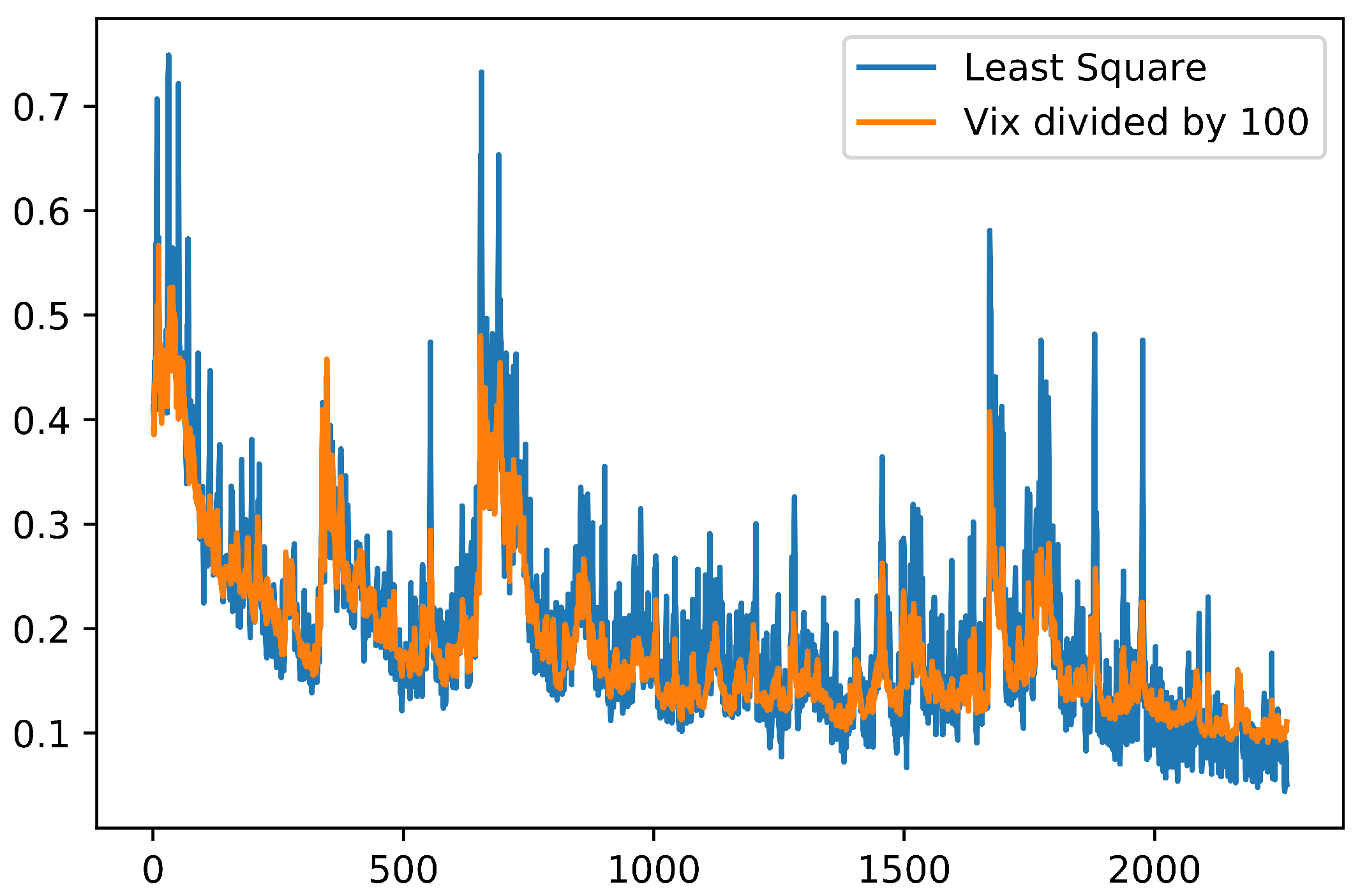
The implied volatility time series ${\widehat{\sigma }}_t$ is shown in Figure 1 (blue line). In the same figure, we also plot the corresponding values of the VIX index (orange line) as a check on whether the ${\widehat{\sigma }}_t$ estimate is reliable. To be able to plot the VIX in the same graph, we had to bring it the same scale as ${\widehat{\sigma }}_t$, so we divided it by 100. As we observe in Figure 1, the two volatility proxies fluctuate in a similar fashion exhibiting the same trends. However, the proposed volatility estimate, ${\widehat{\sigma }}_t$, has more rough behavior than the VIX, suggesting that it is a better candidate to approximate the instantaneous volatility instead of the expected volatility or an averaged volatility.

3.2. Hurst Index Estimation

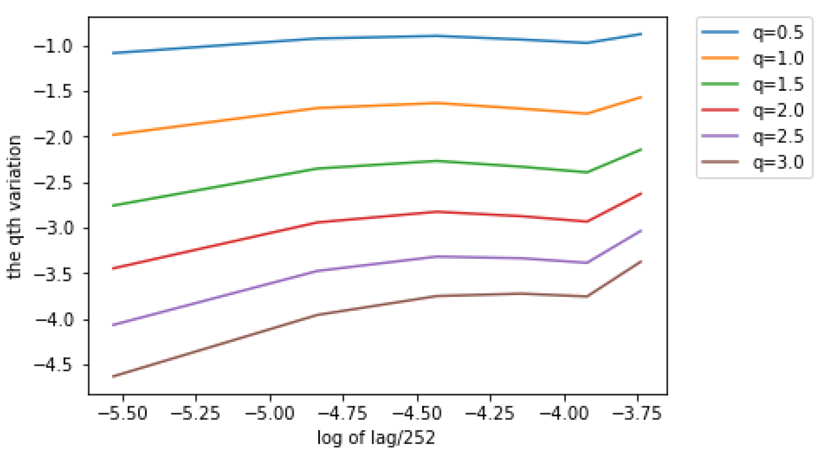
Using the implied volatility process obtained in Section 3.1, we apply the Hurst index estimation methods outlined in Section 2.2 to estimate the Hurst parameter. We start by implementing the variogram approach for different orders of the variogram q ranging between 0.5 and 3. For each q, we estimate the variogram, illustrated in Figure 2, and we compute the corresponding Hurst index via Equation (9). From the plot, we observe that the Hurst estimator does not fluctuate much for different values of q.

Detailed results are summarized in

Table 2. Hurst index estimators of the implied volatility process using (a) the variogram method with different orders q of the variogram, (b) the maximum likelihood approach, (c) the non-parametric rescaled range statistic, and (d) the discrete variation estimator.

q Value	Hurst Index Estimation
0.5	0.16436
1	0.16895
1.5	0.17433
2	0.18122
2.5	0.18983
3	0.20007
Method	Hurst index estimation
MLE	0.21669
R/S	0.89243
Variation method	0.78144

, where we also record the maximum likelihood estimator, the rescaled range statistic (10) and the discrete variations estimator (11). From this Table, we first observe that our intuition that the variogram estimator does not change significantly based on q is confirmed, strengthening our belief that this is a reasonable estimator for the roughness of the volatility process. The maximum likelihood estimator is also very close. This is to be expected because the maximum likelihood method can be seen as an extension of the variogram; both methods are based on a linear relationship between the Hurst index and the logarithm of the variogram. On the other hand, the rescaled range and the discrete variations estimators are very different. This difference can be explained by the low frequency of the data we are working with. In fact, both the R/S and the variation-based estimators are consistent when the sampling frequency goes to 0, which means that they are asymptotically biased for low-frequency observations making them better suited for high-frequency data.

Summarizing the results in this section, we observe that the implied volatility process obtained from Section 3.1 exhibits a rough behavior, even when low-frequency options data are used. We can also conclude that when low-frequency observations are available, one should prefer either the variogram or the maximum likelihood method for estimating the Hurst parameter, since the other two are consistent when the sampling frequency tends to zero.

3.3. The Roughness of VIX

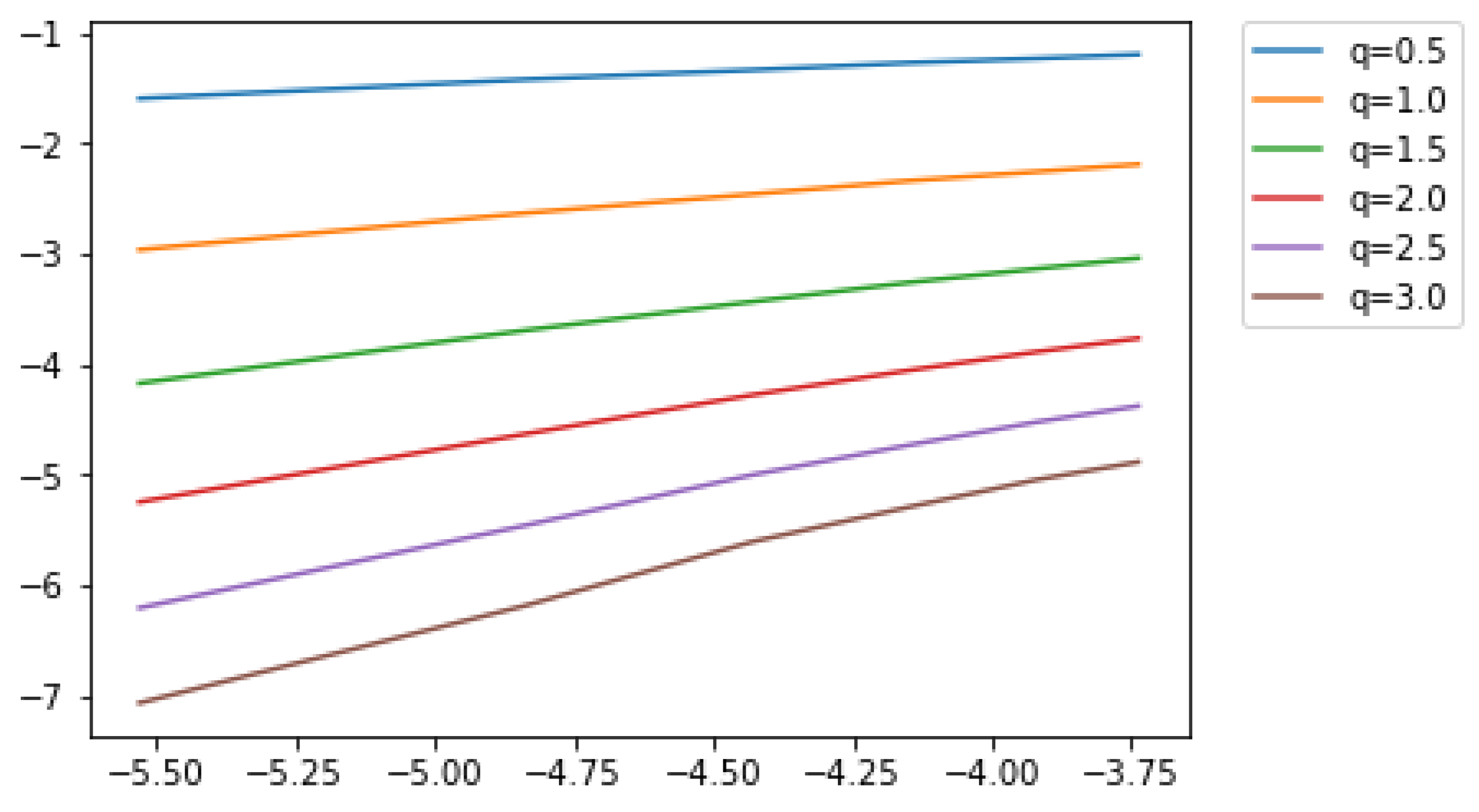
We also want to use the same approach to estimate the Hurst parameter based on the VIX index, which is a volatility proxy quite frequently used in the literature. So, we repeat the same process as before, focusing only on the variogram and the maximum likelihood method. The q-order variograms for the same range of qs are plotted in Figure 3 and the point estimators are summarized in

Table 3. Hurst index estimators of the VIX using (a) the variogram method with different orders q of the variogram, and (b) the maximum likelihood approach.

q Value/Method	Hurst Index Estimation
0.5	0.44485
1	0.43217
1.5	0.42296
2	0.41633
2.5	0.41264
3	0.41254
MLE	0.40889

.

Both methods yield very similar estimators of the Hurst index for the VIX, which are around 0.42, a value significantly higher than 0.21, which is the estimated H obtained using the implied volatility process. This suggests that the roughness of the underlying volatility is better captured via our proposed implied volatility proxy. As expected, the VIX is much less rough since it reflects people’s expectations of averaged future volatility.

3.4. Is the Hurst Index Constant over Time?

In this last section of the results, we investigate whether the Hurst index can be assumed to be constant over a long period of time. Therefore, we split the data into different years and estimate the Hurst index for every year. The results are summarized in

Table 4. Hurst index estimators based on the implied volatility process via the variogram and maximum likelihood methods for each year between 2009 and 2017. For the variogram method, we included the range of the estimators for the different qs.

Year	Estimates by the Variation-Based Method	MLE
2009	0.08–0.14	0.1467
2010	0.17–0.19	0.2446
2011	0.088–0.107	0.1829
2012	0.02–0.036	0.1132
2013	0.135–0.15	0.1739
2014	0.22–0.30	0.3149
2015	0.20–0.30	0.2943
2016	0.218–0.255	0.25485
2017	0.194–0.203	0.21327

.

From Table 4, we conclude that the Hurst index is always on the rougher end, fluctuating year-to-year between 0.02 and 0.30. This is a very wide range of Hurst index values that leads to significant differences when it comes to pricing. To verify the validity of these regression-based estimators, we also perform two tests: the Jarque–Bera test (abbr. JB test) and the Breusch–Pagan test (abbr. BP test). These results are summarized in

Table 5. Validity of variogram-based estimators: Jarque–Bera and Breusch–Pagan tests for the time series from 2 January 2009 to 31 December 2017. All p-values are statistically insignificant validating that the assumptions are satisfied.

q Value	Jarque–Bera Test Statistics	Jarque–Bera Test p-Value	Breusch–Pagan Test Statistics	Breusch–Pagan Test p-Value
0.5	0.55682	0.75699	0.30500	0.58076
1	0.56691	0.75318	0.22542	0.63493
1.5	0.56931	0.75227	0.12210	0.72677
2	0.56657	0.75330	0.04690	0.82855
2.5	0.56097	0.75541	0.00891	0.92480
3	0.55721	0.75684	0.00019	0.98900

. Since all p-values are not statistically significant, we conclude that the assumptions of the variogram method are satisfied. In

Table 6. Validity of variogram-based estimators: Jarque–Bera and Breusch–Pagan tests for the time series in 2014. All p-values are statistically insignificant validating that the assumptions are satisfied.

q Value	Jarque–Bera Test Statistics	Jarque–Bera Test p-Value	Breusch–Pagan Test Statistics	Breusch–Pagan Test p-Value
0.5	0.60818	0.73780	0.14610	0.70228
1	0.64770	0.72336	0.32433	0.56902
1.5	0.60814	0.73781	0.69309	0.40512
2	0.48607	0.78424	1.15858	0.28176
2.5	0.34879	0.83996	1.50670	0.21964
3	0.48800	0.78349	1.66475	0.19696

,

Table 7. Validity of variogram-based estimators: Jarque–Bera and Breusch–Pagan tests for the time series in 2015. All p-values are statistically insignificant validating that the assumptions are satisfied.

q Value	Jarque–Bera Test Statistics	Jarque–Bera Test p-Value	Breusch–Pagan Test Statistics	Breusch–Pagan Test p-Value
0.5	0.54700	0.76071	0.91249	0.33946
1	0.53990	0.76342	0.76327	0.38231
1.5	0.53987	0.76343	0.61092	0.43444
2	0.53987	0.76342	0.55604	0.45585
2.5	0.53724	0.76443	0.67565	0.41108
3	0.56444	0.75411	1.00119	0.31702

,

Table 8. Validity of variogram-based estimators: Jarque–Bera and Breusch–Pagan tests for the time series 2016. All p-values are statistically insignificant validating that the assumptions are satisfied.

q Value	Jarque–Bera Test Statistics	Jarque–Bera Test p-Value	Breusch–Pagan Test Statistics	Breusch–Pagan Test p-Value
0.5	0.59922	0.74111	0.17432	0.67630
1	0.61319	0.73595	0.16395	0.68554
1.5	0.53098	0.76683	0.84132	0.35902
2	0.49933	0.77906	1.25441	0.26271
2.5	0.73162	0.69363	1.3733	0.24124
3	1.24946	0.53540	1.37195	0.24148

and

Table 9. Validity of variogram-based estimators: Jarque–Bera and Breusch–Pagan tests for the time series 2017. All p-values are statistically insignificant validating that the assumptions are satisfied.

q Value	Jarque–Bera Test Statistics	Jarque–Bera Test p-Value	Breusch–Pagan Test Statistics	Breusch–Pagan Test p-Value
0.5	0.25395	0.88075	0.34714	0.55573
1	0.48277	0.78554	0.27510	0.59993
1.5	0.59027	0.74443	0.06219	0.80307
2	0.61923	0.73373	0.00923	0.92345
2.5	0.57036	0.75187	0.18706	0.66538
3	0.45779	0.79541	0.42340	0.51524

, we summarize the detailed results performed for each year separately. The conclusion remains the same that the variogram method assumptions are satisfied.

4. Discussion and Conclusions

In this paper, our main contribution is the use of a new framework to extract an implied volatility process to be used as a proxy for estimating the roughness of the underlying volatility. As we discussed in Section 2.1, the new proxy is obtained by solving an optimization problem, (5), using aggregated option trading data and their corresponding sensitivities. When applied to S&P 500 data, the implied volatility process is reliable, exhibiting similar trends to the VIX index.

Furthermore, we study various methods for estimating the Hurst index, which is a parameter that characterizes the roughness/smoothness of the underlying process. When applied to our new implied volatility proxy, we observe a rough behavior, even when using low-frequency observations, adding value to a common finding in the literature that rough volatility is typically observed in the context of high-frequency trading. This observation shows that it is important to incorporate the roughness of the volatility into the pricing model, even when the trading happens at lower frequencies. Finally, when investigating different ranges of data to estimate the Hurst index, we observe that H is a piecewise constant, which implies that it should be modeled locally.

References

- Aggarwal, Reena, Carla Inclan, and Ricardo Leal. 1999. Volatility in emerging equity markets. Journal of Financial and Quantitative Analysis 34: 33–55. [Google Scholar] [CrossRef]
- Aït-Sahalia, Yacine, and Robert Kimmel. 2007. Maximum likelihood estimation of stochastic volatility models. Journal of Financial Economics 83: 413–52. [Google Scholar] [CrossRef]
- Ait-Sahalia, Yacine, Yubo Wang, and Francis Yared. 2001. Do option markets correctly price the probabilities of movement of the underlying asset. Journal of Econometrics 102: 67–110. [Google Scholar] [CrossRef]
- Alòs, Elisa, and Yan Yang. 2017. A fractional heston model with h > 1/2. Stochastics 89: 384–99. [Google Scholar] [CrossRef]
- Andersen, Torben G., and Tim Bollerslev. 1997. Intraday periodicity and volatility persistence in financial markets. Journal of Empirical Finance 4: 115–58. [Google Scholar] [CrossRef]
- Andersen, Torben G., Tim Bollerslev, Francis X. Diebold, and Paul Labys. 2001. The distribution of realized exchange rate volatility. Journal of the American Statistical Association 96: 42–55. [Google Scholar] [CrossRef]
- Avallaneda, Marco, Craig Friedman, Richard Holmes, and Dominick Samperi. 1997. Calibrating volatility surfaces via relative-entropy minimization. Applied Mathematical Finance 4: 37–64. [Google Scholar] [CrossRef]
- Barndorff-Nielsen, Ole E., and Neil Shephard. 2002. Econometric analysis of realized volatility and its use in estimating stochastic volatility models. Journal of the Royal Statistical Society: Series B (Statistical Methodology) 64: 253–80. [Google Scholar] [CrossRef]
- Bennedsen, Mikkel. 2020. Semiparametric estimation and inference on the fractal index of gaussian and conditionally gaussian time series data. Econometric Reviews 39: 875–903. [Google Scholar] [CrossRef]
- Beran, Jan, Yuanhua Feng, Sucharita Ghosh, and Rafal Kulik. 2016. Long-Memory Processes. Berlin: Springer. [Google Scholar]
- Breidt, F. Jay, Nuno Crato, and Pedro De Lima. 1998. The detection and estimation of long memory in stochastic volatility. Journal of Econometrics 83: 325–48. [Google Scholar] [CrossRef]
- Carr, Peter, and Liuren Wu. 2016. Analyzing volatility risk and risk premium in option contracts: A new theory. Journal of Financial Economics 120: 1–20. [Google Scholar] [CrossRef]
- Chow, Victor, Wanjun Jiang, and Jingrui Victoria Li. 2018. Does Vix Truly Measure Return Volatility? SSRN 2489345. Available online: https://www.worldscientific.com/doi/abs/10.1142/9789811202391_0040 (accessed on 1 March 2018).
- Chronopoulou, Alexandra, and Frederi G. Viens. 2012. Estimation and pricing under long-memory stochastic volatility. Annals of Finance 8: 379–403. [Google Scholar] [CrossRef]
- Coeurjolly, Jean-François. 2001. Estimating the parameters of a fractional brownian motion by discrete variations of its sample paths. Statistical Inference for Stochastic Processes 4: 199–227. [Google Scholar] [CrossRef]
- Coleman, Thomas, Yuying Li, and Arun Verma. 1999. Reconstructing the optimal volatility surface. Journal of Computational Finance 2: 77–102. [Google Scholar] [CrossRef]
- Comte, Fabienne, and Eric Renault. 1998. Long memory in continuous-time stochastic volatility models. Mathematical Finance 8: 291–323. [Google Scholar] [CrossRef]
- Comte, Fabienne, Laure Coutin, and Eric Renault. 2012. Affine fractional stochastic volatility models. Annals of Finance 8: 337–78. [Google Scholar] [CrossRef]
- Cox, John C., Jonathan E. Ingersoll, Jr., and Stephen A. Ross. 1985. An intertemporal general equilibrium model of asset prices. Econometrica: Journal of the Econometric Society 53: 363–84. [Google Scholar] [CrossRef]
- Da Fonseca, José, and Wenjun Zhang. 2019. Volatility of volatility is (also) rough. Journal of Futures Markets 39: 600–11. [Google Scholar] [CrossRef]
- Ding, Zhuanxin, Clive W. J. Granger, and Robert F. Engle. 1993. A long memory property of stock market returns and a new model. Journal of Empirical Finance 1: 83–106. [Google Scholar] [CrossRef]
- Dumas, Bernard, Jeff Fleming, and Robert E. Whaley. 1997. Implied volatility functions, empirical tests. Journal of Finance 53: 2059–106. [Google Scholar] [CrossRef]
- Fouque, Jean-Pierre, George Papanicolaou, and K. Ronnie Sircar. 2000. Derivatives in Financial Markets with Stochastic Volatility. Cambridge: Cambridge University Press. [Google Scholar]
- Fukasawa, Masaaki, Tetsuya Takabatake, and Rebecca Westphal. 2019. Is volatility Rough? arXiv arXiv:1905.04852. [Google Scholar]
- Garman, Mark B. 1976. A General Theory of Asset Valuation under Diffusion State Processes. Available online: https://ideas.repec.org/p/ucb/calbrf/50.html (accessed on 1 March 2018).
- Garnier, Josselin, and Knut Sølna. 2017. Correction to black–scholes formula due to fractional stochastic volatility. SIAM Journal on Financial Mathematics 8: 560–88. [Google Scholar] [CrossRef]
- Gatheral, Jim. 2006. The Volatility Surface: A Practitioner’s Guide. Hoboken: Wiley and Sons. [Google Scholar]
- Gatheral, Jim, Thibault Jaisson, and Mathieu Rosenbaum. 2018. Volatility is rough. Quantitative Finance 18: 933–49. [Google Scholar] [CrossRef]
- Hull, John, and Alan White. 1987. The pricing of options on assets with stochastic volatilities. The Journal of Finance 42: 281–300. [Google Scholar] [CrossRef]
- Hurst, Harold Edwin. 1951. Long-term storage capacity of reservoirs. Transactions of the American Society of Civil Engineers 116: 770–99. [Google Scholar] [CrossRef]
- Jacod, Jean. 2019. Estimation of volatility in a high-frequency setting: A short review. Decisions in Economics and Finance 42: 351–85. [Google Scholar] [CrossRef]
- Kristensen, Dennis. 2010. Nonparametric filtering of the realized spot volatility: A kernel-based approach. Econometric Theory 26: 60–93. [Google Scholar] [CrossRef]
- Livieri, Giulia, Saad Mouti, Andrea Pallavicini, and Mathieu Rosenbaum. 2018. Rough volatility: Evidence from option prices. IISE Transactions 50: 767–76. [Google Scholar] [CrossRef]
- Lo, A. W. 1991. Long memory in stock prices. Econometrica 59: 1279–313. [Google Scholar] [CrossRef]
- Mandelbrot, Benoit B., and John W. Van Ness. 1968. Fractional brownian motions, fractional noises and applications. SIAM Review 10: 422–37. [Google Scholar] [CrossRef]
- Medvedev, Alexey, and Olivier Scaillet. 2007. Approximation and calibration of short-term implied volatilities under jump-diffusion stochastic volatility. The Review of Financial Studies 20: 427–59. [Google Scholar] [CrossRef]
- Szczygielski, Jan Jakub, and Chimwemwe Chipeta. 2023. Properties of returns and variance and implications for time series modeling: Evidence from south africa. Modern Finance 1: 35–55. [Google Scholar] [CrossRef]
- Tudor, Ciprian A., and Frederi Viens. 2008. Variations of the fractional brownian motion via malliavin calculus. Australian Journal of Mathematics 13. [Google Scholar]
- Xiu, Dacheng. 2010. Quasi-maximum likelihood estimation of volatility with high frequency data. Journal of Econometrics 159: 235–50. [Google Scholar] [CrossRef]
- Zhang, Lan, Per A. Mykland, and Yacine Aït-Sahalia. 2005. A tale of two time scales: Determining integrated volatility with noisy high-frequency data. Journal of the American Statistical Association 100: 1394–411. [Google Scholar] [CrossRef]
- Zhou, Bin. 1996. High-frequency data and volatility in foreign-exchange rates. Journal of Business & Economic Statistics 14: 45–52. [Google Scholar]
Figure 1.
The implied volatility time series (blue line) obtained after solving the optimization problem in (5), for the period between 2 January 2009 and 31 December 2017. The VIX for the same period (divided by 100) is superimposed for comparison purposes.
Figure 2.
Plot of qth order variogram obtained based on the implied volatility process against the logarithm of the lag. The Hurst index estimator is the slope of these lines, and based on this figure, we observe that the Hurst estimator (slope of the lines) does not fluctuate much for different values of q.
Figure 3.
Plot of qth order variogram obtained based on the VIX index against the logarithm of the lag. The Hurst index estimator is the slope of these lines, and based on this figure, we observe that the Hurst estimator does not fluctuate much for different values of q.