

Artificial Intelligence Techniques for Bankruptcy Prediction of Tunisian Companies: An Application of Machine Learning and Deep Learning-Based Models


Abstract
:1. Introduction
2. Related Literature
3. Statistical, Machine Learning and Deep Learning Techniques
3.1. Linear Discriminant Analysis (LDA)
3.2. Logistic Regression (LR)
3.3. Decision Trees (DT)
3.4. Support Vector Machine (SVM)
3.5. Random Forests (RF)
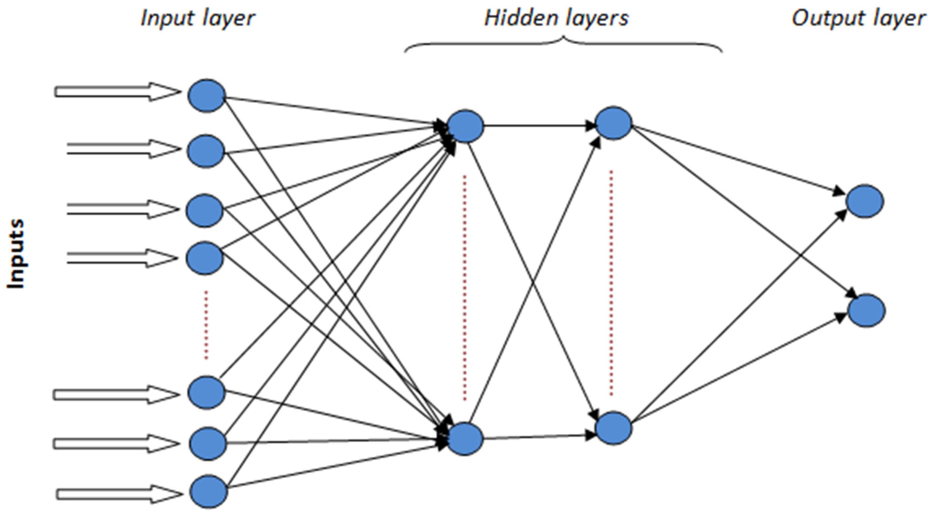
3.6. Deep Neural Network (DNN)
4. Data
5. Empirical Investigation
5.1. Predictive Performance Measures
5.1.1. Accuracy Rate
5.1.2. F1 Score
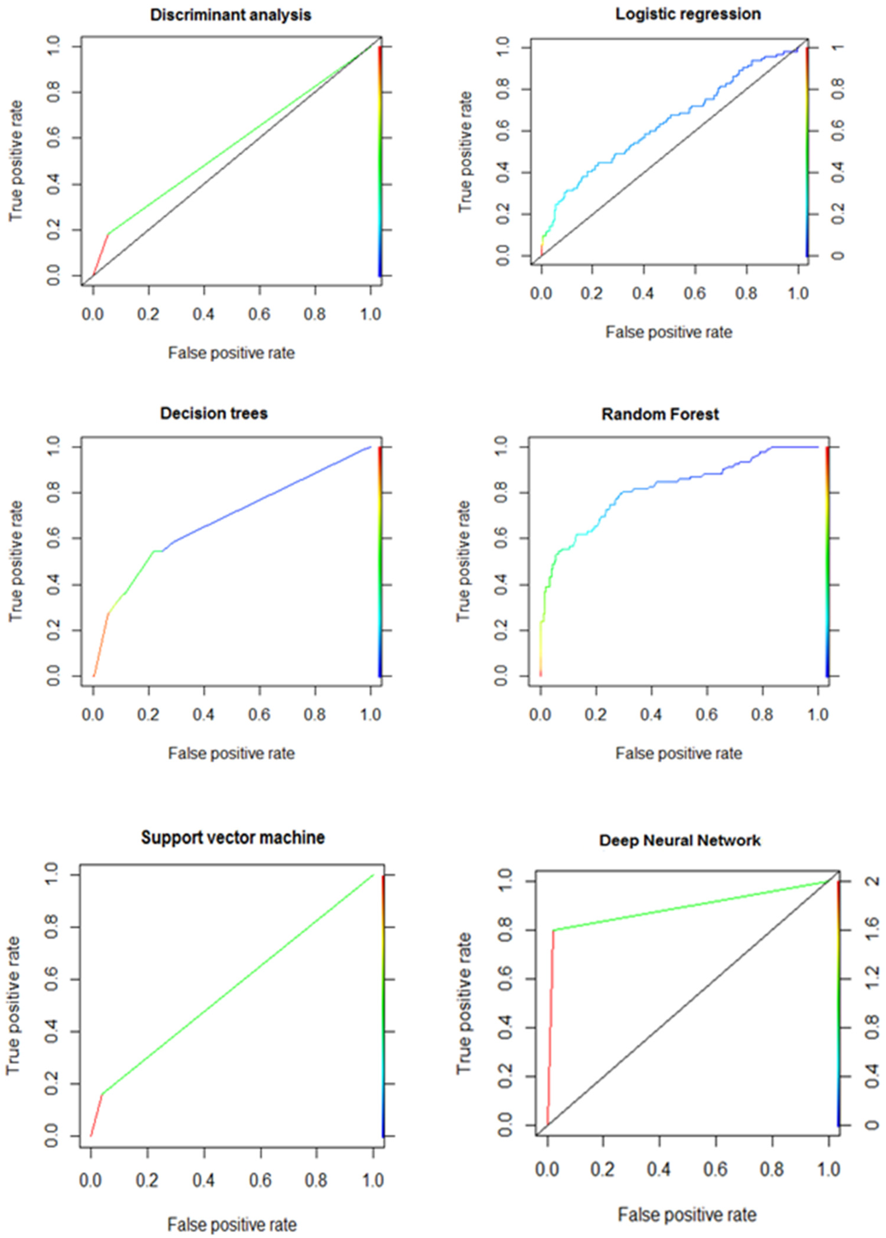
5.1.3. AUC
5.2. Results &Discussion
6. Conclusions
Author Contributions
Funding
Data Availability Statement
Conflicts of Interest
References
- Addo, Peter Martey, Dominique Guegan, and Bertrand Hassani. 2018. Credit Risk Analysis Using Machine and Deep Learning Models. Risks 6: 38. [Google Scholar] [CrossRef]
- Altman, Edward I. 1968. Financial ratios, discriminant analysis, and the prediction of corporate bankruptcy. Journal of Finance 23: 589–609. [Google Scholar] [CrossRef]
- Altman, Edward I., Giancarlo Marco, and Franco Varetto. 1994. Corporate distress diagnosis: Comparisons using linear discriminant analysis and neural networks (the Italian experience). Journal of Banking and Finance 18: 505–29. [Google Scholar] [CrossRef]
- Anandarajan, Murugan, Picheng Lee, and Asokan Anandarajan. 2004. Bankruptcy Prediction Using Neural Networks. Business Intelligence Techniques 11: 117–32. [Google Scholar]
- Aoki, Shigeo, and Yukio Hosonuma. 2004. Bankruptcy Prediction Using Decision Tree. In The Application of Econophysics. Tokyo: Springer, pp. 299–302. [Google Scholar]
- Atiya, Amir. 2001. Bankruptcy Prediction for Credit Risk Using Neural Networks: A Survey and New Results. IEEE Transactions on Neural Networks 12: 929–35. [Google Scholar] [CrossRef] [PubMed]
- Aydin, Nezir, Nida Sahin, Muhammet Deveci, and Dragan Pamucar. 2022. Prediction of financial distress of companies with artificial neural networks and decision trees models. Machine Learning with Applications 10: 100432. [Google Scholar] [CrossRef]
- Barboza, Flavio, Herbert Kimura, and Edward Altman. 2017. Machine learning models and bankruptcy prediction. Expert Systems with Applications 83: 405–17. [Google Scholar] [CrossRef]
- Beaver, William H. 1966. Financial ratios as predictors of failure. Journal of Accounting Research 4: 71–111. [Google Scholar] [CrossRef]
- Begović, Sanja Vlaović, and Ljiljana Bonić. 2020. Developing a model to predict corporate bankruptcy using decision tree in the Republic of Serbia. Facta Universitatis, Series: Economics and Organization 17: 127–39. [Google Scholar] [CrossRef]
- Ben Jabeur, Sami, and Vanessa Serret. 2023. Bankruptcy prediction using fuzzy convolutional neural networks. Research in International Business and Finance 64: 101–844. [Google Scholar] [CrossRef]
- Biau, Gérard. 2012. Analysis of a random forests model. The Journal of Machine Learning Research 13: 1063–95. [Google Scholar]
- Bragoli, Daniela, Camilla Ferretti, Piero Ganugi, Giovanni Marseguerra, Davide Mezzogori, and Francesco Zammori. 2022. Machine-learning models for bankruptcy prediction: Do industrial variables matter? Spatial Economic Analysis 17: 156–77. [Google Scholar] [CrossRef]
- Breiman, Leo. 2001. Random Forests. Machine Learning 45: 5–32. [Google Scholar] [CrossRef]
- Chang, Chih-Chung, and Chih-Jen Lin. 2011. LIBSVM: A library for support vector machines. ACM Transactions on Intelligent Systems and Technology 2: 1–27. [Google Scholar] [CrossRef]
- Chen, Mu-Yen. 2011. Bankruptcy prediction in firms with statistical and intelligent techniques and a comparison of evolutionary computation approaches. Computers and Mathematics with Applications 62: 4514–24. [Google Scholar] [CrossRef]
- Clement, Claudiu. 2020. Machine learning in bankruptcy prediction—A review. Journal of Public Administration, Finance and Law 17: 178–96. [Google Scholar]
- Cristianini, Nello, and John Shawe-Taylor. 2000. An Introduction to Support Vector Machines and Other Kernel-Based Learning Methods. Cambridge: Cambridge University Press, pp. 1–189. [Google Scholar]
- Davalos, Sergio, Fei Leng, Ehsan Feroz, and Zhiyan Cao. 2014. Designing an if-then rules-based ensemble of heterogeneous bankruptcy classifiers: A genetic algorithm approach. Intelligent Systems in Accounting, Finance and Management 21: 129–53. [Google Scholar] [CrossRef]
- Deakin, Edward B. 1972. A discriminant analysis of predictors of business failure. Journal of Accounting Research 10: 167–79. [Google Scholar] [CrossRef]
- Dellepiane, Umberto, Michele Di Marcantonio, Enrico Laghi, and Stefania Renzi. 2015. Bankruptcy Prediction Using Support Vector Machines and Feature Selection during the Recent Financial Crisis. International Journal of Economics and Finance 7: 182–95. [Google Scholar] [CrossRef]
- Deng, Li, and Dong Yu. 2014. Deep Learning: Methods and Applications. Foundations and Trends in Signal Processing 7: 197–387. [Google Scholar] [CrossRef]
- Efron, Bradley. 1975. The efficiency of logistic regression compared to normal discriminant analysis. Journal American Statistical Society 7: 892–98. [Google Scholar] [CrossRef]
- Elhoseny, Mohamed, Noura Metawa, Gabro Sztano, and Ibrahim M. El-hasnony. 2022. Deep Learning-Based Model for Financial Distress Prediction. Annals of Operations Research 11: 1–23. [Google Scholar] [CrossRef] [PubMed]
- Fisher, Ronald. 1933. The use of multiple measurements in taxonomic problems. Annals of Eugenics 7: 179–88. [Google Scholar] [CrossRef]
- Gelfand, Saul B., C. S. Ravishankar, and Edward J. Delp. 1991. An iterative growing and pruning algorithm for classification tree design. IEEE Transaction on Pattern Analysis and Machine Intelligence 13: 163–74. [Google Scholar] [CrossRef]
- Gergely, Fejér-Király. 2015. Bankruptcy Prediction: A Survey on Evolution, Critiques, and Solutions. Acta Universitatis Sapientiae, Economics and Business 3: 93–108. [Google Scholar]
- Gunn, Steve. 1998. Support Vector Machines for Classification and Regression. Technical Report. Southampton: University of Southampton. [Google Scholar]
- Gurnani, Ishika, Febryan Stefanus Tandian, and Maria Susan Anggreainy. 2021. Predicting Company Bankruptcy Using Random Forest Method. Paper presented at IEEE 2nd International Conference on Artificial Intelligence and Data Sciences (AiDAS), IPOH, Malaysia, September 8–9; pp. 1–5. [Google Scholar]
- Hamdi, Manel. 2012. Prediction of Financial Distress for Tunisian Firms: A Comparative Study between Financial Analysisand Neuronal Analysis. Business Intelligence Journal 5: 374–82. [Google Scholar]
- Hamdi, Manel, and Sami Mestiri. 2014. Bankruptcy Prediction for Tunisian Firms: An Application of Semi-Parametric Logistic Regression and Neural Networks Approach. Economics Bulletin 34: 133–43. [Google Scholar]
- Härdle, Wolfgang Karl, Rouslan Moro, and Dorothea Schäfer. 2005. Predicting Bankruptcy with Support Vector Machines. In Statistical Tools for Finance and Insurance. Berlin and Heidelberg: Springer. [Google Scholar]
- Hearst, Marti A., Susan T. Dumais, Edgar Osuna, John Platt, and Bernhard Scholkopf. 1998. Support vector machines. IEEE Intelligent System 13: 18–28. [Google Scholar] [CrossRef]
- Heo, Junyoung, and Jin Yong Yang. 2014. AdaBoost based bankruptcy forecasting of Korean construction companies. Applied Soft Computing 24: 494–99. [Google Scholar] [CrossRef]
- Hosaka, Tadaaki. 2019. Bankruptcy prediction using imaged financial ratios and convolutional neural networks. Expert Systems with Applications 117: 287–99. [Google Scholar] [CrossRef]
- Joshi, Shreya, Rachana Ramesh, and Shagufta Tahsildar. 2018. A Bankruptcy Prediction Model Using Random Forest. Paper presented at IEEE Second International Conference on Intelligent Computing and Control Systems (ICICCS), Madurai, India, June 14–15. [Google Scholar]
- Kamruzzaman, M. M., and Omar Alruwaili. 2022. AI-based computer vision using deep learning in 6G wireless networks. Computers and Electrical Engineering 102: 108233. [Google Scholar] [CrossRef]
- Kim, Myoung-Jong, and Ingoo Han. 2003. The Discovery of Experts’ Decision Rules from Qualitative Bankruptcy Data Using Genetic Algorithms. Expert Systems with Application 25: 637–46. [Google Scholar] [CrossRef]
- Kim, Phil. 2017. MATLAB Deep Learning: With Machine Learning, Neural Networks and Artificial Intelligence, 1st ed. New York: A Press Book. 151p. [Google Scholar]
- Kuizinienė, Dovilė, Tomas Krilavičius, Robertas Damaševičius, and Rytis Maskeliūnas. 2022. Systematic Review of Financial Distress Identification using Artificial Intelligence Methods. Applied Artificial Intelligence 36: 2138124. [Google Scholar] [CrossRef]
- Kumar, Ravi, and Vadlamani Ravi. 2007. Bankruptcy prediction in banks and firms via statistical and intelligent techniques—A review. European Journal of Operational Research 180: 1–28. [Google Scholar] [CrossRef]
- LeCun, Yann, Yoshua Bengio, and Geoffrey Hinton. 2015. Deep learning. Nature 521: 436–44. [Google Scholar] [CrossRef] [PubMed]
- Mai, Feng, Shaonan Tian, Chihoon Lee, and Ling Ma. 2019. Deep learning models for bankruptcy prediction using textual disclosures. European Journal of Operational Research 274: 743–58. [Google Scholar] [CrossRef]
- Martono, Niken Prasasti, and Hayato Ohwada. 2023. Financial Distress Model Prediction Using Machine Learning: A Case Study on Indonesia’s Consumers Cyclical Companies. In Machine Learning and Principles and Practice of Knowledge Discovery in Databases. Cham: Springer, vol. 1753. [Google Scholar]
- Matin, Rastin, Casper Hansen, Christian Hansen, and Pia Mølgaard. 2019. Predicting distresses using deep learning of text segments in annual reports. Expert Systems with Applications 132: 199–208. [Google Scholar] [CrossRef]
- Máté, Domicián, Hassan Raza, and Ishtiaq Ahmad. 2023. Comparative Analysis of Machine Learning Models for Bankruptcy Prediction in the Context of Pakistani Companies. Risks 11: 176. [Google Scholar] [CrossRef]
- Mestiri, Sami, and Manel Hamdi. 2013. Credit Risk Prediction: A Comparative Study between Logistic Regression and Logistic Regression with Random Effects. International Journal of Management Science and Engineering Management 7: 200–4. [Google Scholar] [CrossRef]
- Narvekar, Aditya, and Debashis Guha. 2021. Bankruptcy prediction using machine learning and an application to the case of the COVID-19 recession. Data Science in Finance and Economics 1: 180–95. [Google Scholar] [CrossRef]
- Noh, Seol-Hyun. 2023. Comparing the Performance of Corporate Bankruptcy Prediction Models Based on Imbalanced Financial Data. Sustainability 15: 4794. [Google Scholar] [CrossRef]
- Noviantoro, T., and J. P. Huang. 2021. Comparing machine learning algorithms to investigate company financial distress. Review of Business, Accounting & Finance 1: 454–79. [Google Scholar]
- Odom, Marcus D., and Ramesh Sharda. 1990. A neural network model for bankruptcy prediction. Paper presented at the International Joint Conference on Neural Networks, San Diego, CA, USA, June 17–21; Alamitos: IEEE Press, vol. 2, pp. 163–68. [Google Scholar]
- Ohlson, James A. 1980. Financial Ratios and the Probabilistic Prediction of Bankruptcy. Journal of Accounting Research 18: 109–31. [Google Scholar] [CrossRef]
- Pang, Su-Juan. 2006. Application of Logistic Regression Model in Credit Risk Analysis. Mathematics in Practice and Theory 9: 129–37. [Google Scholar]
- Park, Min Sue, Hwijae Son, Chongseok Hyun, and Hyung Ju Hwang. 2021. Explainability of Machine Learning Models for Bankruptcy Prediction. IEEE Access 9: 124887–99. [Google Scholar] [CrossRef]
- Pepe, Margaret Sullivan. 2000. Receiver operating characteristic methodology. Journal of the American Statistical Association 95: 308–11. [Google Scholar] [CrossRef]
- Ptak-Chmielewska, Aneta, and Anna Matuszyk. 2020. Application of the random survival forests method in the bankruptcy prediction for small and medium enterprises. Argumenta Oeconomica 1: 127–42. [Google Scholar] [CrossRef]
- Qu, Yi, Pei Quan, Minglong Lei, and Yong Shi. 2019. Review of bankruptcy prediction using machine learning and deep learning techniques. Procedia Computer Science 162: 895–9. [Google Scholar] [CrossRef]
- Quinlan, J. Ross. 1986. Induction of decision trees. Machine Learning 1: 81–106. [Google Scholar] [CrossRef]
- Roy, Tanmoy, Marwala Tshilidzi, and Snehashish Chakraverty. 2021. Chapter 12—Speech emotion recognition using deep learning. In New Paradigms in Computational Modeling and Its Applications. Cambridge: Academic Press, pp. 177–87. [Google Scholar]
- Sabir, Zulqurnain, Muhammad Asif Zahoor Raja, Sharifah E. Alhazmi, Manoj Gupta, Adnène Arbi, and Isa Abdullahi Baba. 2022. Applications of artificial neural network to solve the nonlinear COVID-19 mathematical model based on the dynamics of SIQ. Journal of Taibah University for Science 16: 874–84. [Google Scholar] [CrossRef]
- Schmidhuber, Jürgen. 2015. Deep learning in neural networks: An overview. Neural Networks 61: 85–117. [Google Scholar] [CrossRef] [PubMed]
- Shetty, Shekar, Mohamed Musa, and Xavier Brédart. 2022. Bankruptcy Prediction Using Machine Learning Techniques. Journal of Risk and Financial Management 15: 35. [Google Scholar] [CrossRef]
- Shin, Kyung-Shik, Taik Soo Lee, and Hyun-jung Kim. 2005. An Application of Support Vector Machines in Bankruptcy Prediction Model. Expert Systems and Applications 28: 127–35. [Google Scholar] [CrossRef]
- Shin, Kyung-Shik, and Yong-Joo Lee. 2002. A genetic algorithm application in bankruptcy prediction modeling. Expert Systems with Applications 23: 321–28. [Google Scholar] [CrossRef]
- Suganyadevi, S., V. Seethalakshmi, and Krishnasamy Balasamy. 2022. A review on deep learning in medical image analysis. International Journal of Multimedia Information Retrieval 11: 19–38. [Google Scholar] [CrossRef]
- Vapnik, Vladimir Naumovich, and Vlamimir Vapnik. 1998. The Nature of Statistical Learning Theory. New York: Springer. [Google Scholar]
- Vuk, Miha, and Tomaz Curk. 2006. Roc curve, lift chart and calibration plot. Organization Science 3: 89–108. [Google Scholar] [CrossRef]
- Walczak, Steven, and Narciso Cerpa. 2003. Artificial Neural Networks. In Encyclopedia of Physical Science and Technology, 3rd ed. Cambridge: Academic Press. [Google Scholar]
- Wilson, Rick L., and Ramesh Sharda. 1994. Bankruptcy Prediction Using Neural Networks. Decision Support Systems 11: 545–57. [Google Scholar] [CrossRef]
- Xie, Ying, Linh Le, Yiyun Zhou, and Vijay V. Raghavan. 2018. Chapter 10—Deep Learning for Natural Language Processing. In Handbook of Statistics. Amsterdam: Elsevier, vol. 38, pp. 317–28. [Google Scholar]
- Zibanezhad, Elahe, Daryush Foroghi, and Amirhassan Monadjemi. 2011. Applying decision tree to predict bankruptcy. Paper presented at IEEE International Conference on Computer Science and Automation Engineering, Shanghai, China, June 10–12; pp. 165–69. [Google Scholar]
- Zou, Jinming, Yi Han, and Sung-Sau So. 2008. Overview of Artificial Neural Networks. In Artificial Neural Networks. Totowa: Humana Press, vol. 458, pp. 14–22. [Google Scholar]
- Zweig, Mark, and Gregory Campbell. 1993. Receiver-operating characteristic (ROC) plots: A fundamental evaluation tool in clinical medicine. Clinical Chemistry 39: 561–77. [Google Scholar] [CrossRef]


| Author(s) | Model(s) | Type of Input Variables | Sampling Period | Performance Criteria Used | Conclusion(s) |
|---|---|---|---|---|---|
| Addo et al. (2018) |
| 10 financial variables | 2016–2017 |
|
|
| Hosaka (2019) |
| 133 financial items | 2002–2016 |
|
|
| Noviantoro and Huang (2021) |
| 96 financial indicators | 1999–2009 |
|
|
| Shetty et al. (2022) |
| Three financial ratios: the return on assets, the current ratio, and the solvency ratio | 2002–2012 |
|
|
| Elhoseny et al. (2022) |
| 179 financial attributes | 2000–2013 |
|
|
| Ben Jabeur and Serret (2023) |
| 17 financial variables | 2014–2017 |
|
|
| Noh (2023) |
| 13 financial variables | 2012–2021 |
|
|
| Duration credit to the customer | Permanent capital turnover | ||
| Gross margin rate | Return on permanent capital | ||
| Operating margin rate | Rate of long-term debt | ||
| Ratio of personnel expenses | Ratio of financial independence | ||
| Net margin rate | Total debt ratio | ||
| Asset turnover | Immobilisation coverage by equity capital | ||
| Equity turnover | The long- and medium-term debt capacity | ||
| Economic profitability | Ratio of financial expenses | ||
| rate of return on assets | Financial expenses/total debt | ||
| Operating profitability of total assets | Working capital ratio | ||
| Gross economic profitability | Relative liquidity ratio | ||
| Net economic profitability | Quick ratio | ||
| Rate of return on equity | |||
| Predicted class “0” | Predicted class “1” | |
| Real class“0” | True positive (T0) | False positive (F1) |
| Real class“1” | False negative (F0) | True negative (T1) |
| Models | Accuracy Rate | F1-Score | AUC | Rank |
|---|---|---|---|---|
| Linear Discriminant Analysis (LDA) | 80.9% | 0.890 | 0.574 | 5 |
| Logistic Regression (LR) | 85.8% | 0.922 | 0.633 | 3 |
| Decision Trees (DT) | 74.3% | 0.838 | 0.675 | 6 |
| Random Forest (RF) | 88.2% | 0.933 | 0.815 | 2 |
| Support Vector Machine (SVM) | 84.8% | 0.910 | 0.563 | 4 |
| Deep Neural Network (DNN) | 93.6% | 0.964 | 0.888 | 1 |
Disclaimer/Publisher’s Note: The statements, opinions and data contained in all publications are solely those of the individual author(s) and contributor(s) and not of MDPI and/or the editor(s). MDPI and/or the editor(s) disclaim responsibility for any injury to people or property resulting from any ideas, methods, instructions or products referred to in the content. |
© 2024 by the authors. Licensee MDPI, Basel, Switzerland. This article is an open access article distributed under the terms and conditions of the Creative Commons Attribution (CC BY) license (https://creativecommons.org/licenses/by/4.0/).
Share and Cite
Hamdi, M.; Mestiri, S.; Arbi, A. Artificial Intelligence Techniques for Bankruptcy Prediction of Tunisian Companies: An Application of Machine Learning and Deep Learning-Based Models. J. Risk Financial Manag. 2024, 17, 132. https://doi.org/10.3390/jrfm17040132
Hamdi M, Mestiri S, Arbi A. Artificial Intelligence Techniques for Bankruptcy Prediction of Tunisian Companies: An Application of Machine Learning and Deep Learning-Based Models. Journal of Risk and Financial Management. 2024; 17(4):132. https://doi.org/10.3390/jrfm17040132
Chicago/Turabian StyleHamdi, Manel, Sami Mestiri, and Adnène Arbi. 2024. "Artificial Intelligence Techniques for Bankruptcy Prediction of Tunisian Companies: An Application of Machine Learning and Deep Learning-Based Models" Journal of Risk and Financial Management 17, no. 4: 132. https://doi.org/10.3390/jrfm17040132