Avoiding barren plateaus in the variational determination of geometric entanglement

The current generation of quantum processors has been described as noisy intermediate-scale quantum (NISQ) devices, which are characterized by a number of qubits in the hundreds, low gate fidelity, short coherence times, and limited qubit connectivity [1]. These features preclude the use of error-correcting techniques [2, 3] and the implementation of deep quantum circuits, severely limiting its usability. Despite this adverse scenario, the family of variational quantum algorithms (VQAs) [4–6] emerges as a promising candidate to solve problems of practical interest in NISQ processors while offering advantages over classical computers. VQAs are hybrid quantum-classical algorithms where a cost function is efficiently evaluated on a quantum processor and is optimized using classical optimization routines. This approach is used by variational quantum eigensolvers [7], quantum approximate optimization algorithms [8], and quantum neural networks [9–11], finding applications in quantum chemistry [12–14], finances [15–18], and quantum tomography [19–25], among others.

Recently, VQAs have been applied to estimate the entanglement of quantum states [26–28]. Among them, the variational determination of geometric entanglement (VDGE) [29] estimates the geometric measure of entanglement (GME) of pure multi-qubit quantum states $|\Psi\rangle$. The GME is an entanglement monotone given by the distance between $|\Psi\rangle$ and its nearest fully separable state $|\Phi\rangle$. It was first introduced for bipartite pure states [30] and later generalized to multipartite systems [31]. The GME has been used to study the distinguishability of multipartite quantum states using local operations [32], quantum phase transitions in spin models [33], Grover's search algorithm [34], and entanglement witnesses [35]. VDGE minimizes the infidelity between $|\Psi\rangle$ and a parameterized separable state $|\alpha (\boldsymbol{\theta})\rangle$ to calculate the GME. This procedure requires only local unitary operations on each qubit, so the implementation in a quantum processor is direct, requiring only circuits of depth 1. VDGE has been shown to be experimentally feasible, with experiments up to five qubits on IBM's quantum processors.

Numerical simulations of VDGE for 25 qubit GHZ and W states have been performed, showing the convergence of the algorithm even in such a high dimension [29]. However, the simulations consider initial conditions close to the optimum. With random initial conditions, VDGE exhibits a clear lack of convergence. This is a common problem of current implementations of VQAs called the barren plateau (BP) phenomenon [36], which is characterized by a lack of convergence due to a gradient of the cost function with a vanishing average and a standard deviation that decreases exponentially with the number of qubits by, for example, a global cost function [37] or the presence of noise [38]. The BP strongly limits the applicability of most VQAs, so the search for techniques to avoid BP has become a significant problem today. It has been shown that BPs can be avoided in some VQA by employing a local cost function instead of a global one [37, 39–41], using better initial parameters for the optimization [42, 43], detecting the BPs with classical shadows [44], reducing the expressiveness of the parametric circuit [45], including mid-circuit measurements [46], using quantum annealing [47], geometric quantum machine learning [48], overparametrization [49], or improved gradient methods [50]. Despite the advances on this topic, there is no general indication to avoid BP in a generic VQA, and moreover, it is not clear which technique will help to avoid BPs in VDGE.

In this article, we propose a method to avoid BP in VDGE. We call this the improved VDGE (iVDGE) method, which complements VDGE by adding a previous stage to find better initial parameters in the search space so that VDGE does not fall into the BP. In this initial stage, the global infidelity is replaced by the average of two-qubit infidelities, that is, a local function, which is subsequently minimized. We show that this average bounds the infidelity, so minimizing it also minimizes the global infidelity. Furthermore, the value of these bounds can be efficiently obtained through an unbiased estimator, whose error decreases with the number of qubits. Using this local function instead of a global one drives the optimization out of the flat landscape associated with the BP with a higher probability than the standard VDGE. Our approach establishes an alternative strategy to avoid BP in the case of global functions and thus complements the arsenal of existing proposals [37, 39–41].

We carried out exhaustive numerical simulations to test the performance of iVDGE and compare it with VDGE. Simulations for random states up to six qubits show that iVDGE speeds up convergence and is more resource-efficient than VDGE. Simulations for states of 18 qubits show that while iVDGE converges near the optimum, VDGE exhibits BP. Noisy numerical simulations with seven qubits for several resources show that BPs appear with a much smaller probability in iVDGE than in VDGE, being 10% and 71%, respectively for a sample of 8192 shots. We experimentally test and corroborate our findings by running iVDGE and VDGE for a seven-qubit GHZ state on the IBM quantum processors [51].

2.1. GME determination by VDGE

The GME $E_\Psi$ of an n-qubit quantum state $|\Psi \rangle$ is defined through the optimization problem

$$\begin{align} E_\Psi = \min_{|\Phi\rangle \in \textrm{Pro} \left(\mathcal{H}\right)} I_\Psi\left(\Phi\right), \end{align} \tag{ 1 }$$

where

$$\begin{equation} I_\Psi\left(\Phi\right) = 1- | \langle \Psi |\Phi\rangle |^2 \end{equation} \tag{ 2 }$$

is the infidelity between two n-qubit pure states and $\textrm{Pro} \left( \mathcal{H} \right) = \{|\Phi_1 \rangle \otimes \cdots \otimes |\Phi_n\rangle: |\Phi_j \rangle \in \mathcal{H}_{j} \}$ is the subset of pure product states of the Hilbert space $\mathcal{H} = \bigotimes_{j = 1}^n \mathcal{H}_j$ of n qubits. Thereby, $E_\Psi$ corresponds to the minimal infidelity between the state $|\Psi\rangle$ and the set $\textrm{Pro} \left( \mathcal{H} \right)$ [35].

The VDGE attempts to find $E_\Psi$ by optimizing the infidelity over a variational ansatz. For this, we define the Hamiltonian

$$\begin{align} H_\textrm{G} = \unicode{x1D7D9} - |0 \rangle \langle 0 |^{\otimes n} \end{align} \tag{ 3 }$$

and the variational ansatz

$$\begin{align} |\alpha \left(\boldsymbol{\theta}\right)\rangle = U^\dagger \left(\boldsymbol{\theta}\right) |\Psi \rangle. \end{align} \tag{ 4 }$$

Here $U (\boldsymbol{\theta}) = \bigotimes_{j = 1}^n U_j (\boldsymbol{\theta}_j)$, where $U_j (\boldsymbol{\theta}_j)$ is parametric single-qubit unitary operation acting on the jth qubit. Thus, the cost function

$$\begin{align} I_\Psi\left(\boldsymbol{\theta}\right) = 1 - \langle \Psi | U \left(\boldsymbol{\theta}\right) |0 \rangle \langle 0 |^{\otimes n} U^\dagger \left(\boldsymbol{\theta}\right) | \Psi \rangle \end{align} \tag{ 5 }$$

now depends on the parameters of ansatz and can be cast as

$$\begin{equation} I_\Psi\left(\boldsymbol{\theta}\right) = \langle H_\textrm{G} \rangle_{\boldsymbol{\theta}} = \langle \alpha \left(\boldsymbol{\theta}\right) | H_\textrm{G} |\alpha \left(\boldsymbol{\theta}\right)\rangle. \end{equation} \tag{ 6 }$$

This can be estimated by repeatedly preparing the n-qubit state $|\Psi \rangle$, applying the circuit that implements $U (\boldsymbol{\theta})$, and measuring on the computational basis.

The infidelity $I_\Psi(\boldsymbol{\theta})$ is minimized by an optimization method running on a classical computer. Typical choices for the optimization method are the simultaneous perturbation stochastic approximation (SPSA) method [52] and, more recently, its complex version CSPSA [21]. These methods require in each iteration the estimation of $I_\Psi(\boldsymbol{\theta})$ in two different points of the optimization space. Therefore, after a prescribed number of iterations, VDGE provides an estimate $\hat E_\Psi$ of GME. The minimization of GME is, however, a challenging problem since the optimization landscape might exhibit many local minima. This is usually overcome by repeating the optimization several times with different initial conditions to obtain a set of estimates $\{\hat{E}_\Psi^k \}$. The final estimate is given by the minimum over this set, that is $\hat{E}_\Psi = \min_k\{\hat{E}_\Psi^k \}$.

Numerical simulations of VDGE for 25 qubit GHZ and W states exhibit the BP phenomenon [29]. This occurs because for a n-qubit system both the infidelity $I_\Psi(\boldsymbol{\theta})$ and its gradient vanish exponentially with the number of qubits when the initial parameters are randomly chosen [53]. One alternative to overcome this problem is to have a better initial condition, which can be obtained, for instance, by resorting to a priori information [42, 43] about the solution. Another alternative is to overcome the sampling noise by employing more than $O(2^n)$ measurement shots, which leads to accurate evaluations of $I_\Psi(\boldsymbol{\theta})$ and its gradient. This, however, does not guarantee avoiding the BP, and moreover, the exponential scaling of the shot number makes the algorithm unfeasible.

2.2. iVDGE

The BP phenomenon may arise due to inadequate cost functions [39, 41]. Specifically, cost functions based on global observables can lead to exponentially vanishing gradients, needing an exponential number of shots to estimate the gradient accurately. In particular, as discussed in [37], cost functions with local observables may result in a slower vanishing of the gradient, thereby avoiding the BP. To prevent the BP phenomenon from adversely affecting the performance of VDGE, we replace the global infidelity equation (5) with a local cost function, the gradient of which does not vanish exponentially with the number of qubits (see appendix A for details). We define this function as the expectation value of the local Hamiltonian

$$\begin{equation} H_\mathrm{L} = \unicode{x1D7D9} - \frac{2}{n\left(n-1\right)} \sum_{\substack{i, j = 1 \\ i < j}}^n \Pi_{i j}, \end{equation} \tag{ 7 }$$

where each operator Π_ij acts as a rank-1 projector on qubits i and j, that is,

$$\begin{align} \Pi_{i j} = |0_i \rangle \langle 0_{i}| \otimes |0_j \rangle \langle 0_j|, \end{align} \tag{ 8 }$$

and as an identity operator on any other qubit. The Hamiltonian $H_\mathrm{L}$ is constructed such that $| 0\rangle^{\otimes n}$ is its ground state and its expected value is given by the average of the two-qubit infidelities

$$\begin{align} I_{ij}\left(\boldsymbol{\theta}_i, \boldsymbol{\theta}_j\right) = 1 - \mathrm{Tr} \left( \rho_{ij} \left(\boldsymbol{\theta}_i, \boldsymbol{\theta}_j\right) \; \Pi_{ij} \right), \end{align} \tag{ 9 }$$

where $\rho_{i,j}$ is the reduced density matrix of qubits i and j from state $|\alpha (\boldsymbol{\theta})\rangle$.

The expectation value $\langle H_\mathrm{L} \rangle_{\boldsymbol{\theta}} = \langle \alpha (\boldsymbol{\theta}) | H_\mathrm{L} |\alpha (\boldsymbol{\theta})\rangle$ can be used to obtain the following upper and lower bounds of the infidelity (see appendix B for details).

$$\begin{align} \langle H_\mathrm{L} \rangle_{\boldsymbol{\theta}} \unicode{x2A7D} I_\Psi \left(\boldsymbol{\theta}\right) \unicode{x2A7D} \left\lfloor \frac{n}{2} \right\rfloor \langle H_\mathrm{L} \rangle_{\boldsymbol{\theta}}, \end{align} \tag{ 10 }$$

which are tight if and only if $| \Psi \rangle$ is a product state. According to equation (10), it is possible to obtain a first estimate of the GME by minimizing the local function $\langle H_\mathrm{L} \rangle_{\boldsymbol{\theta}}$ instead of the global function $\langle H_\mathrm{G} \rangle_{\boldsymbol{\theta}}$.

The expectation value of the Hamiltonian $H_\mathrm{L}$ can be cast in the form

$$\begin{equation} \langle H_\mathrm{L} \rangle_{\boldsymbol{\theta}} = \frac{1}{\vert \mathcal{G} \vert} \sum_{g\in\mathcal{G}} X_g, \end{equation} \tag{ 11 }$$

where

$$\begin{equation} X_g = \frac{1}{\lfloor n/2 \rfloor}\sum_{\left(i,j\right)\in g} I_{ij} \left(\boldsymbol{\theta}_i,\boldsymbol{\theta}_j\right) \end{equation} \tag{ 12 }$$

and the set $\mathcal{G}$ contains all groups g of partitions of n qubits formed by non-overlapping pairs of qubits. This suggests that the expectation value $\langle H_\mathrm{L}\rangle_{\boldsymbol{\theta}}$ can be evaluated by sampling X_g uniformly on the set $\mathcal{G}$. For a given group g the evaluation of the infidelities in X_g can be performed efficiently since the measurements are local and can be carried out in parallel. To keep resource usage to a minimum, we randomly select a single X_g as an estimator of $\langle H_\mathrm{L} \rangle_{\boldsymbol{\theta}}$. This estimator is unbiased, that is, $\mathbb{E}(X_g) = \langle H_\mathrm{L}\rangle_{\boldsymbol{\theta}}$, and its mean square error (MSE) is bounded and decreases inversely proportional with the number of qubits (see appendix C for details),

$$\begin{equation} \textrm{MSE}\left(X_g \right) \unicode{x2A7D} \frac{n-1}{\left(n-2\right)\left(n-3\right)} . \end{equation} \tag{ 13 }$$

The algorithm that we propose, which we call iVDGE, arises from concatenating the following two stages: (i) the minimization of the expectation value of the local Hamiltonian $H_\mathrm{L}$ to obtain a first estimate of the GME, and (ii) the execution of a standard VDGE, that minimizes the expectation value of the global Hamiltonian $H_\mathrm{G}$, but using as initial guess the estimator obtained from the stage (i). The concatenation of these steps allows us to avoid BPs and accurately estimate the GME.

Stage (i) is performed as follows:

• (a)  
  Split the n qubits in a partition of $\lfloor n/2 \rfloor$ pairs (i, j) at random, plus a single qubit if n is odd, or equivalently, sample a single group $g\in\mathcal{G}$ of non-overlapping pairs of qubits.
• (b)  
  For each pair (i, j) in the partition, perform a single iteration of a classical optimization method to minimize the corresponding local infidelity (9). This is equivalent to minimizing the expected value of the local Hamiltonian $H_\mathrm{L}$.
• (c)  
  Repeat steps (a) and (b) a predefined number $N_\mathrm{L}$ of times according to a classical optimization method.

Let us note that stage (i) is only used to escape from the BP. As we are only estimating two-qubit functions, we require a number of shots that is polynomial in the number of qubits to obtain a useful estimation of the gradient. Outside the BP, the minimization of the global function converges faster than the minimization of the local function. Here we need a number of shots at least proportional to $1 /(1 - E_{\Psi})$, as we must be able to calculate the gradient of the infidelity around the value of the $E_{\Psi}$.

Selecting the classical optimization method is fundamental to obtaining good performance with iVDGE. Particularly, we chose the CSPSA method [21] (see appendix F). This is a stochastic optimization algorithm that works over complex parameters. Due to that, in our case, θ is a complex vector of 2n elements, where each pair of parameters defines a single qubit state. Other optimization algorithms might give a better performance. In algorithm 1, we present the pseudocode of the iVDGE when CSPSA is used as the classical optimization method.

Algorithm 1. iVDGE algorithm.
Input: quantum state Ψ, number of local iterations $N_\mathrm{L}$, number of global iterations $N_\mathrm{G}$
Initialization: parameters $\boldsymbol{\theta}_0 = (\theta_0^1,\theta_0^2,\dots ,\theta_0^n)\in \mathbb{C}^{2\times n}$
for $k = 1,\ldots, N_\mathrm{L}+N_\mathrm{G}$ do
if $k\unicode{x2A7D} N_\mathrm{L}$ then
Set a pair-wise partition $\left\{( i_l,j_l) \right\}_{l = 1}^{\lfloor n/2\rfloor}$ of $\{1,2,\dots,n\}$
for $l = 1,\ldots ,\lfloor n/2\rfloor$ do
Compute CSPSA gradient $\nabla I_{i_l,j_l}$
$\left( \theta_k^{i_l} \theta_k^{j_l} \right) = \left(\theta_{k-1}^{i_l} \theta_{k-1}^{j_l}\right) - a_k \nabla I_{i_l},{j_l}\left(\theta^{i_l}_{k-1},\theta^{j_l}_{k-1}\right)$
end
else
Compute CSPSA gradient $\nabla I_{\Psi}(\theta_{k-1})$
$\boldsymbol{\theta}_k = \boldsymbol{\theta}_{k-1} - a_k\nabla I_{\Psi}(\boldsymbol{\theta_{k-1}})$
end
end

The iVDGE method might still get trapped in local optima. To avoid them, we run the optimization several times starting from different separable initial states to obtain a set of possible estimators of the GME, and keep the best value obtained as the final estimator.

2.3. Numerical simulations

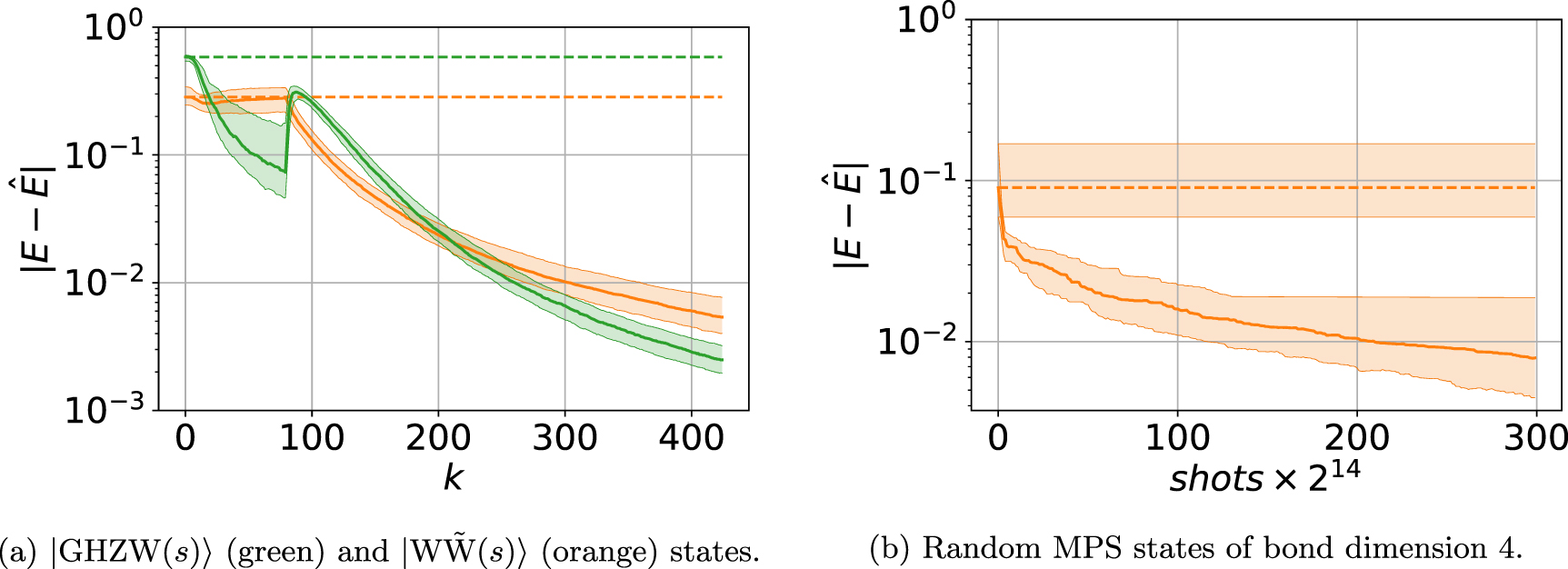
The first numerical test shows the effectiveness of replacing the local Hamiltonian $H_\mathrm{L}$ with a random Hamiltonian at each iteration of the optimization algorithm. We generate 100 random matrix product states (MPSs), each with a bond dimension of 16 and 10 qubits. Solid curves in figure 1 show the median difference $|E-\hat{E}|$ between the exact GME E and the estimated GME $\hat{E}$ values. The green curve denotes optimization over the function $\langle H_\mathrm{L}\rangle_\theta$ followed by the global function, whereas the orange curve represents optimization over the local randomized function X_g followed by the global function. In both cases, the first stage comprises 80 local iterations, measured using 512 shots, and the second stage is composed of 295 global iterations employing 8196 shots. The exact value of the GME was calculated using the Basin-hopping optimization algorithm [54] (see appendix E). As figure 1 clearly shows, using the local random function X_g in the early stages of the algorithm leads to a higher convergence rate than when using the function $\langle H_\mathrm{L}\rangle_\theta$, which even exhibits stagnation in the late stages of the algorithm. According to equation (12), the minimization of X_g corresponds to the minimization of $n/2$ independent terms, since g is a set of disjoint pairwise partition of the set of qubits. Thereby, for a given iteration k, we have to calculate $n/2$ independent gradients, and then update the parameters of $n/2$ independent functions. Since these functions only depend on two qubits, they can be evaluated to a high precision with a small number of shots. On the other hand, according to equation (11), the minimization of $\langle H_\mathrm{L}\rangle_\theta$ requires minimizing a sum of $n(n-1)/2$ local functions. These are not independent anymore and thus the optimization problem cannot be split into a sum of two-qubit optimization problems. The sum of this large quantity of two-qubit functions increases the variance in the estimation of $\langle H_\mathrm{L}\rangle_\theta$. For a fixed, small number of shots, the evaluation of X_g has a smaller error than the evaluation of $\langle H_\mathrm{L}\rangle_\theta$, which is more favorable for the optimization algorithm.

Zoom In Zoom Out Reset image size

In our second test, we consider simulations with random initial conditions for a small number of qubits and compare iVDGE and VDGE. We generate a set of 100 pure states randomly chosen according to a Haar-uniform distribution for 3, 4, 5, and 6 qubits. For each state, we estimate the GME using both methods. For iVDGE, the first stage is implemented with 80 iterations, using 512 shots to simulate each measurement of the infidelity. The second stage is executed with 295 iterations and using 8192 shots per infidelity evaluation. The first stage uses a total of shots equal to that used in five iterations of the second stage. On the other hand, VDGE is implemented using 300 iterations with 8192 shots per infidelity evaluation. Therefore, our implementations of iVDGE and VDGE use the same number of shots. To avoid local optima, this procedure is repeated five times for each randomly generated state in both methods, and the minimum GME value obtained is the final GME estimate. We also numerically compute the exact value of the GME for each of the randomly generated states through the Basin-hopping optimization algorithm (see appendix E).

The comparison between the performances of iVDGE and VDGE is shown in figure 2. The orange (green) curve represents the median of the difference $|E - \hat{E}|$ between E, the exact GME value, and $\hat{E}$, the values obtained through iVDGE (VDGE) as a function of the number of accumulated shots. Shaded areas correspond to interquartile ranges. As figure 2 indicates, iVDGE achieves faster convergence and higher accuracy than VDGE in all four cases. As the number of qubits increases, the interquartile ranges of iVDGE and VDGE do not intersect and the estimation precision of GME decreases and presents flattening, the latter being less pronounced for the iVDGE method.

Zoom In Zoom Out Reset image size

To comparatively study the performance of iVDGE and VDGE in the high qubit number regime, where the BP phenomenon is expected to arise, we perform simulations with particular quantum states since the calculation of the GME for arbitrary states in this regime becomes unfeasible [53]. We resort to the GHZ, W, and $\tilde{\mathrm{W}}$ states for n qubits given by the expressions.

$$\begin{align} | \textrm{GHZ} \rangle & = \frac{1}{\sqrt{2}}\left( |00 \cdots 0 \rangle + |11 \cdots 1\rangle\right), \end{align} \tag{ 14 }$$

$$\begin{align} |\textrm{W} \rangle & = \frac{1}{\sqrt{n}}( | 10\cdots0 \rangle + | 01\cdots0 \rangle +\cdots +|0\cdots01\rangle, \end{align} \tag{ 15 }$$

$$\begin{align} |\tilde{\mathrm{W}} \rangle & = \frac{1}{\sqrt{n}}( | 01\cdots1 \rangle + | 10\cdots1 \rangle +\cdots +|1\cdots10\rangle. \end{align} \tag{ 16 }$$

These states have GME values of 0.5 for the GHZ state and $1 - [(n-1)/n)]^{n-1}$ for W and $\tilde{\mathrm{W}}$ states [35]. For superpositions of the form

$$\begin{align} |\textrm{GHZW} \left(s\right) \rangle = \sqrt{s} | \textrm{GHZ}\rangle + \sqrt{1 - s}| \textrm{W} \rangle, \end{align} \tag{ 17 }$$

or

$$\begin{align} |\textrm{W}\tilde{\mathrm{W}} \left(s\right) \rangle = \sqrt{s} | \textrm{W}\rangle + \sqrt{1 - s}| \tilde{\mathrm{W}} \rangle, \end{align} \tag{ 18 }$$

with $s \in [0, 1]$, the GME is optimized by a symmetric separable state [55], that is, $|\Phi \rangle \otimes \dots \otimes |\Phi \rangle$. This reduces the optimization space to only two parameters, making it easier to evaluate the exact value of the GME using classical optimization techniques.

Figure 3 exhibits the value of the GME obtained with VDGE and iVDGE for the states $|\textrm{GHZW} (s) \rangle$ and $|\textrm{W}\tilde{\mathrm{W}} (s) \rangle$ as a function of s and for n = 18 qubits. For each state and value of $s = 0.05m$ with $m = 0, 1, \dots, 20$, VDGE and iVDGE are executed with five randomly selected initial conditions, and the minimum value of GME is selected as an estimate. This procedure is repeated 100 times. Orange stars represent the median value obtained using iVDGE with 80 iterations in the first stage and 295 iterations in the second stage. The infidelities were approximated with 512 and 8192 shots, respectively. Green circles represent the median value obtained using VDGE with 300 iterations, evaluating the infidelity with 8192 shots. The solid blue curve represents the exact value of the GME (see appendix E). Shaded areas correspond to interquartile ranges, which are extremely narrow. Even with such scarce resources, iVDGE converges to the GME, while VDGE never escapes a value other than one. This suggests that the BP phenomenon is present in VDGE, while iVDGE can avoid it, converging to the exact value.

Zoom In Zoom Out Reset image size

Figure 4(a) allows us to analyze the convergence of iVDGE from a different perspective using the data from the previous simulation. This figure displays the median error $|E - \hat{E}|$ calculated on the set of 100 GME estimates for all 21 values of s for $|\textrm{GHZW} (s) \rangle$ states (green) and $|\textrm{W}\tilde{\mathrm{W}} (s) \rangle$ states (orange), as a function of the number of iterations. Solid and dashed lines display the median of iVDGE and VDGE, respectively. Shaded areas correspond to interquartile ranges. VDGE and iVDGE start at the same point in the parameter space. In the first 80 iterations, iVDGE tries to find a good starting point for global optimization in the second stage. For the orange curve, we see that although the distance from the optimum does not improve significantly in the first stage, at the beginning of the second stage, iVDGE is effectively outside the BP and also converges. For the green curve, we see that the distance from the optimum increases when iVDGE switches to the second stage. This behavior might be controlled by fine-tuning the hyper-parameters of the optimization algorithm. Nevertheless, iVDGE does not enter the BP again and converges with good accuracy. The solid (dashed) line in figure 4(b) shows the median error $|E - \hat{E}|$ calculated on a set of 100 random MPS states of 18 qubits and bond dimension 4 using iVDGE (VDGE). We use 80 iterations in the first stage of VDGE and 295 iterations in the second stage. As can be seen from this figure, VDGE cannot provide a value of the GME, while iVDGE shows a systematic decrease of the median error toward the exact value. As in the previous cases, iVDGE also manages to escape from the BP.

Zoom In Zoom Out Reset image size

To study the ability of the iVDGE algorithm to bypass noise-induced BPs [38], we performed noisy simulations for both VDGE and iVDGE using limited resources and the noise model of IBM Quantum system ibm_oslo, which includes one- and two-qubit gate errors as well as measurement errors. The GME of a seven-qubit GHZ state is calculated for 100 randomly generated initial conditions with VDGE and iVDGE, using different numbers of shots. For the VDGE algorithm, we performed 200 iterations, while for the iVDGE algorithm, we performed 80 local iterations plus the required number of global iterations such that the same total number of shots is used in both methods. For example, to match the 200 iterations of VDGE with 8192 shots, iVDGE uses 80 local iterations with 512 shots and 195 global iterations with 8192 shots. On the last iteration, we perform error mitigation using matrix inversion to mitigate the measurement error. Unlike the previous simulations, we do not consider extra repetitions with random initial conditions to avoid local optima. The GME of a GHZ is equal to 0.5, but the state prepared by the circuit has a GME of $0.491\,77$ due to noisy operations that decrease the amount of entanglement. We consider that the algorithm is trapped in a BP if, after the optimization, the GME is still greater than 0.9.

Tables 1 and 2 show the percentage of BPs appearance for a given amount of total shots for the VDGE and iVDGE algorithms, respectively, together with the median estimated GME for the 100 different initial conditions. The simulations show that in the case of VDGE, the BP appearance is approximately independent of the number of shots, where about 70% of the realizations exhibit the BP phenomenon. On the other hand, the BP occurrence for the iVDGE simulations stays relatively low using 512 local shots and up to 1024 global shots but increases rapidly by further reducing the total number of shots. The median GME only changes drastically when using the lowest amount of shots. The iVDGE results show a better convergence compared to the VDGE method and a better median GME for every set of shots.

Table 1. Percentage of BPs appearances and median GME value of a seven-qubit GHZ state with 100 randomly generated initial conditions using the VDGE algorithm with different numbers of shots. For every case, 200 iterations are considered.

VDGE
Global shots	BP %	Median GME
8192	71%	0.9822
4096	69%	0.9855
2048	74%	0.9830
1024	69%	0.9854
512	74%	0.9836
256	73%	0.9866
130	77%	0.9828

Table 2. Percentage of BPs appearances and median GME value of a seven-qubit GHZ state with 100 randomly generated initial conditions using the iVDGE algorithm with different numbers of shots. For every case, 80 iterations are performed on the local stage, while the number of iterations on the global stage is chosen such that the same total number of shots is used in both methods.

iVDGE
Local shots	Global shots	BP %	Median GME
512	8192	10%	0.5322
512	4096	10%	0.5322
512	2048	9%	0.5331
512	1024	9%	0.5407
256	512	16%	0.5516
128	256	20%	0.5951
64	128	39%	0.7698

2.4. Experimental results for seven-qubit GHZ state

Following the results obtained from the noisy simulations, we can observe a BP if we consider a low number of shots compared to the dimension, and check the experimental performance of both algorithms with limited resources using the IBM quantum processor ibm_oslo.

We measure the GME of a seven-qubit GHZ state using iVDGE and VDGE, repeating the procedure 12 times with different initial conditions. For iVDGE, we perform 80 local and 260 global iterations using 128 and 256 shots, respectively, to estimate the infidelities. For VDGE we perform 300 iterations using 256 shots for each measurement of the infidelity. As the performance of the quantum device is affected by various noise sources, we can not generate an ideal GHZ state. Because of this, we perform quantum state tomography using $20\,000$ shots per basis with maximum likelihood estimation [56, 57] using a pure state parameterization and error mitigation [58], obtaining an estimated GHZ state that has fidelity of $0.91 \pm 0.01$ with respect to the ideal GHZ. The GME of the estimated state is obtained using the Basin-hopping optimization algorithm, which leads to a GME value of $0.519 \pm 0.01$.

To estimate the experimental errors of both the fidelity and the GME, we sample 100 times from the probability distribution obtained from measuring every basis for the quantum state tomography and reconstruct a sampled state using maximum likelihood estimation. The error of the fidelity is then given by the standard deviation of the fidelity between the sampled states and the ideal GHZ state, while the error of the GME corresponds to the standard deviation of every GME value of the sampled states after the classical optimization with Basin-hopping.

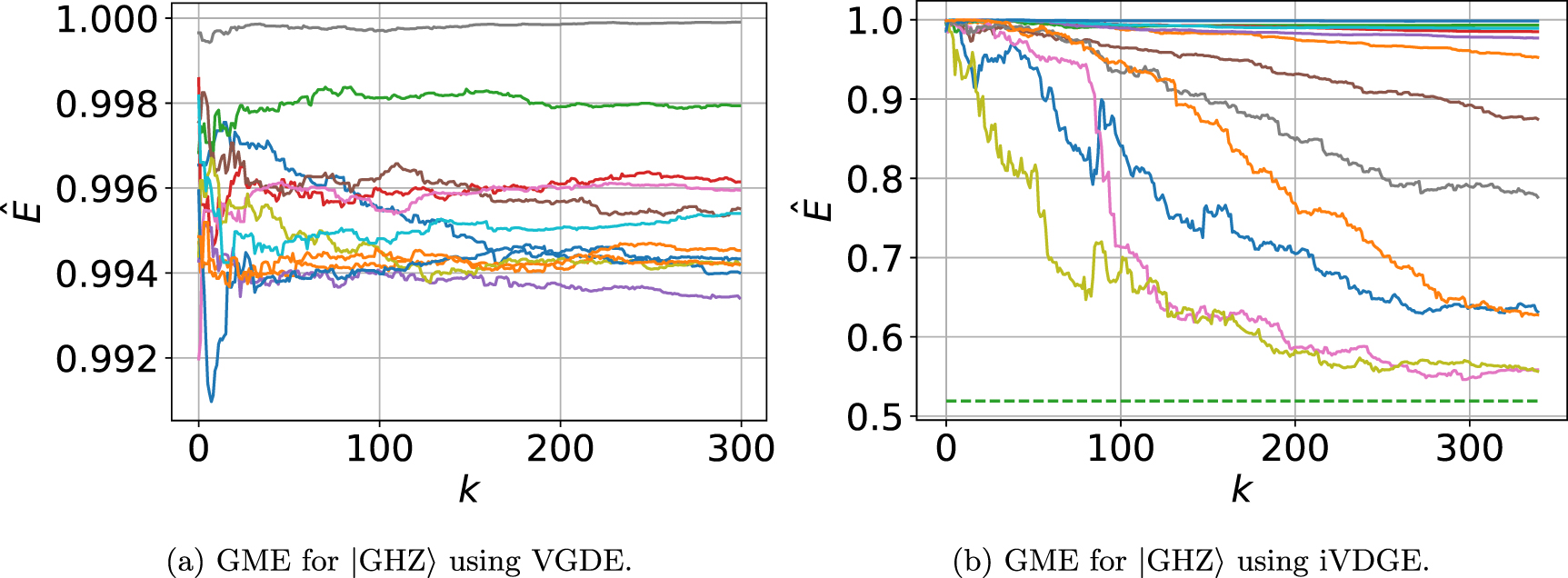
Figure 5 shows the value of the GME for the experimentally estimated GHZ state provided by (a) VDGE and (b) iVDGE as a function of the number of iterations, for 12 independent realizations. The GME is calculated by evaluating the infidelity between the experimentally estimated GHZ state and the separable state provided by VDGE or iVDGE. The dotted line represents the theoretical GME value of 0.519. According to figure 5, of the 12 repetitions of VDGE, not a single one manages to escape the BP, while 5 of the 12 repetitions of iVDGE manage to surpass it, following the criteria defined in our numerical simulations. This percentage of BP appearance is higher than the one expected from the noisy simulations. One possible explanation is that the model does not consider other sources of error, like decoherence, cross-talk between qubits, state preparation error, etc.

Zoom In Zoom Out Reset image size

2.5. Avoiding BPs in other variational algorithms

In this subsection, we discuss other variational problems where our approach to avoid BP could be applied. We can define a family of variational problems using the following global Hamiltonian,

$$\begin{align} H_\mathrm{G} = U\left( \unicode{x1D7D9} - \sum_{k_1\cdots k_n = 0}^1 c_{k_1\cdots k_n}\bigotimes_{j = 1}^{n} | k_j \rangle\langle k_j | \right) U^\dagger, \end{align} \tag{ 19 }$$

with U an unitary matrix, $c_{k_1\cdots k_n}$ real coefficients, and $\{|k_j\rangle \}_{k = 0}^1$ the canonical basis of the jth qubit. The coefficients $c_{k_1\cdots k_n}$ satisfy $0\unicode{x2A7D} c_{k_1\cdots k_n}\unicode{x2A7D} 1$ to bound the expected value of $H_\mathrm{G}$ in the range $0\unicode{x2A7D} \langle H_\mathrm{G} \rangle \unicode{x2A7D} 1$. Notice that we recover the VDGE Hamiltonian, equation (3), for $U = \unicode{x1D7D9}$ and $c_{k_1\cdots k_n} = \delta_{k_10}\cdots\delta_{k_n0}$. Other problems included in this Hamiltonian are the quantum autoencoder [37], the quantum-assisted compiling [39], the variational quantum linear solver [40], and the variational quantum state diagonalization [41].

Similarly to iVDGE, we define the following two-qubit local Hamiltonian

$$\begin{align} H_\mathrm{L} = U\left( \unicode{x1D7D9} - \frac{2}{n\left(n-1\right)}\sum_{\substack{i, j = 1 \\ i < j}}^n\Pi_{ij} \right)U^\dagger, \end{align} \tag{ 20 }$$

with Π_ij the two-qubit operator

$$\begin{align} \Pi_{ij} = \sum_{k_1\cdots k_n = 0}^1 c_{k_1\cdots k_n} | k_i \rangle\langle k_i | \otimes | k_j \rangle\langle k_j |. \end{align} \tag{ 21 }$$

Notice that Π_ij acts as the identity in the other qubits. Let us define h_ij as the expected value of Π_ij on a variational state $\rho(\theta)$, that is

$$\begin{align} h_{ij}\left(\boldsymbol{\theta}\right) = \textrm{Tr}\left( \rho\left(\boldsymbol{\theta}\right) \Pi_{ij} \right). \end{align} \tag{ 22 }$$

Analogously to iVDGE, we define an estimator of the expectation value of the local Hamiltonian $H_\mathrm{L}$ as the average of h_ij over a set of non-overlapping pairs of qubits,

$$\begin{align} \langle H_\mathrm{L} \rangle_\theta = \frac{1}{|\mathcal{G}|}\sum_{g\in\mathcal{G}} X_g, \end{align} \tag{ 23 }$$

with

$$\begin{align} X_g = \frac{1}{\lfloor n/2 \rfloor}\sum_{\left(i,j\right)\in g} h_{ij} \left(\boldsymbol{\theta}\right). \end{align} \tag{ 24 }$$

Following the same strategy as iVDGE, we first optimize the local Hamiltonian to escape from the flat landscape and later use its optimum as the initial condition to optimize the global Hamiltonian.

The main difference between iVDGE and an arbitrary variational problem defined by $H_\mathrm{G}$ lies in the variational ansatz. While iVDGE requires only local gates, equation (4), an arbitrary problem could require several layers of entangling gates, preventing the optimization of the local Hamiltonian $\langle H_\mathrm{L} \rangle_\theta$ by parallel optimizing the two-body reduced functions $h_{ij}(\boldsymbol{\theta})$. Instead, in each iteration of the variational algorithm, we randomly select a set of non-overlapping pairs of qubits $g\in\mathcal{G}$ and use directly X_g as an estimate of $\langle H_\mathrm{L} \rangle_\theta$ to update the parameters. Despite that, we expect our approach's ability to remain as long as the variational ansatz behaves well against BPs [48].

The GME can be evaluated in NISQ devices via the VDGE method. This is done using a parametric quantum circuit which involves local gates only. This allows us to avoid two sources of the BP phenomenon: deep parametric quantum circuits and high levels of noise. However, since the function to be optimized is global, that is, its evaluation requires measurements onto sets of many qubits simultaneously, the BP phenomenon still impairs the performance of VDGE method for a large number of qubits.

In order to avoid the BP phenomenon in the context of the GME we propose the iVDGE method, which adds a previous stage to the VDGE method. This is based on measuring a two-qubit local function, which is the expectation value $\langle H_\mathrm{L} \rangle$ of a two-qubit Hamiltonian, that upper and lower bounds the global function. This suggests optimizing the local function allows us to optimize the global one. The local function is minimized for a fixed number of iterations, producing preliminary parameters used as a starting point for VDGE. The first stage of iVDGE can be efficiently carried out using an unbiased estimator X_g with bounded error of the local function.

We performed several numerical simulations to investigate the performance of iVDGE to estimate the GME and its ability to avoid BP. We start by analyzing both methods for random states in a small number of qubits, as shown in figure 2. Since we are working with a low number of qubits, we can expect both VDGE and iVDGE to converge to the optimum given a suitable number of iterations. Nevertheless, we can see that iVDGE provides a speed-up in the convergence concerning VDGE for a fixed total number of shots. To assess the performance of the methods for a large number of qubits, we conducted simulations involving superpositions of GHZ and W states of 18 qubits, as well as random MPS states. As figures 3 and 4 indicate, the VDGE method stagnates at E = 1, showing the presence of the BP phenomenon. Meanwhile, iVDGE avoids it and successfully converges to the correct value of the GME. Notice that figure 4(a) shows that the first stage of iVDGE does not necessarily provide an accurate estimate for the GME. Nevertheless, the iVDGE method produces a good enough starting point so that the VDGE method will avoid the flat landscape and converge. Finally, we study the efficiency of iVDGE in the presence of noise by simulating a seven-qubit GHZ state using the model of an actual NISQ device so that a noise-induced BP arises. According to table 1, the VDGE method escapes from the BP with a probability of approximately 0.3, which leads to a median GME value of 0.98, far away from the correct GME value of 0.5, in a wide range of global shot number. The scenario in the case of iVDGE, shown in table 2, is drastically different, where iVDGE escapes from the BP and converges to the correct GME value with a high probability of approximately 0.8, even for a low global shot number of 256. This shows that iVDGE not only avoids BPs produced by global objective functions but also avoids noise-induced BPs.

To test the performance of the iVDGE method on the current quantum hardware generation, we conducted experiments on the IBM quantum processor ibm_oslo. We studied the GME of a seven-qubit GHZ state, and to illustrate the difference between the performance of VDGE and iVDGE we chose a low number of shots, such that BP emerges. In particular, we considered a number of 256 shots, which is twice the dimension of the search space. Figure 5 shows the estimated GME value of 12 independent runs, where the VDGE method does not escape the BP, while iVDGE effectively shows that most of the runs escape the BP and even some of them are close to the correct GME value.

For the experimental results, the dimension of the system is $2^7 = 128$. When we start from a random separable state, we can expect that the initial estimated GME for the GHZ will be close to $(1/2)^7 = 1/128$, as any local state has a mean fidelity of $1/2$ when randomly chosen according to the Haar measure [59]. Following the noisy simulations and the size of the problem, we can expect that using only 256 shots to estimate this quantity is insufficient to construct a good approximation of the gradient. This is one of the effects seen in figure 5, where none of the trajectories of VDGE left the BP zone. On the other hand, in the first stage of iVDGE we have 128 shots to estimate fidelities in dimension 4, which can be done with more precision. Then, when we pass to the second stage, 5 of 12 trajectories escape the BP.

Considering the previous discussion, iVDGE is effectively an improvement of VDGE. We have seen that it can avoid the BP phenomena produced by global functions in high dimensional systems and noise-induced BP. Moreover, it provides a speed-up over VDGE in scenarios where the BP phenomenon is not observed. These improvements do not add complexity to the algorithm, as the local function used in the initial stage can be efficiently evaluated, and it employs the same ansatz as VDGE. In our simulations, the number of shots required does not scale exponentially with the number of qubits. Then, we expect an accurate estimate of the GME even in high-dimensional systems.

Our protocol finds direct application in estimating the entanglement of many-body quantum states in current devices. For example, recently, 27 qubits GHZ states [60] and native-graph states [61] have been implemented. The ability of iVDGE to avoid BPs qualifies it as an efficient alternative to certify the entanglement of these states. Moreover, our proposal represents a step forward and complements previous results to handle BPs in variational algorithms. The standard approach is to optimize in the first stage a Hamiltonian composed of single-qubit observables, removing the coupling between the subsystems. In contrast, our approach uses two-qubit observables, so it preserves some of the entanglement structure of the Hamiltonian. This property can be advantageous for problems where entanglement plays a crucial role, such as estimating the ground state of molecules known to be entangled [12]. We also anticipate the applicability of our strategy in variational problems such as quantum autoencoder [37], quantum-assisted compiling [39], variational quantum linear solver [40], and variational quantum state diagonalization [41], as they share similar Hamiltonian definitions with VDGE.

The iVDGE method can be enhanced in various ways. The switch between local and global Hamiltonians is crucial in the performance of the algorithm, so establishing a precise criterion for switching without compromising fidelity is essential. This can be done, for instance, by considering a suitable set of gain coefficients on CSPSA. An alternative approach [41] has been recently suggested, where an adiabatic process is employed instead of abruptly changing the Hamiltonian from local to global. This is done evaluating the Hamiltonian $H_k = (1-\lambda_k)H_\mathrm{L} + \lambda_kH_\mathrm{G}$ in the kth iteration of the optimization, where $\{\lambda_k\}$ is a sequence of positive coefficients such that λ₁ = 0 and $\lambda_{k_{\mathrm{max}}} = 1$. This approach allows us to escape from the flat landscape using the local Hamiltonian in early iterations, while the global Hamiltonian permits precise estimation of GME in later iterations. Furthermore, our protocol is not limited to using two-qubit local Hamiltonians. Adding more stages to the protocol, where local Hamiltonians with more qubits are used, could speed up the method. For example, firstly, optimize over two-qubits local Hamiltonians, then with $n/2$-qubits local Hamiltonians, and in the last stage, carry out a global optimization with n-qubits. These upgrades can enhance the efficiency and accuracy of the protocol, making it a valuable tool for entanglement estimation in many-body quantum systems.

This work was supported by ANID—Millennium Science Initiative Program—ICN17$_-$012. L Z was supported by the Government of Spain (Severo Ochoa CEX2019-000910-S, TRANQI, and European Union NextGenerationEU PRTR-C17.I1), Fundació Cellex, Fundació Mir-Puig and Generalitat de Catalunya (CERCA program). A D was supported by FONDECYT Grants 1231940 and 1230586. M M was supported by ANID-PFCHA/DOCTORADO-NACIONAL/2019-21190958. L P was supported by ANID-PFCHA/DOCTORADO-BECAS-CHILE/2019-772200275, the CSIC Interdisciplinary Thematic Platform (PTI+) on Quantum Technologies (PTI-QTEP+), the CAM/FEDER Project No. S2018/TCS-4342 (QUITEMAD-CM), and the Proyecto Sinérgico CAM 2020 Y2020/TCS-6545 (NanoQuCo-CM).

The data cannot be made publicly available upon publication because no suitable repository exists for hosting data in this field of study. The data that support the findings of this study are available upon reasonable request from the authors.

This section aims to show the exponential decay of the variance of the global cost function as the number of qubits increases and show how our proposed local Hamiltonian solves this. For simplicity, we will consider the separable state $|\Phi \rangle = |\Phi_1 \rangle \otimes \cdots \otimes |\Phi_n\rangle$ as our target state. First, we notice that any single qubit state can be parameterized using the unitary $U(\theta, \phi)$ given by:

$$\begin{equation} U\left(\theta, \phi\right) = \begin{pmatrix} \text{cos} \frac{\theta}{2} & \mathrm{e}^{\mathrm{i} \phi} \text{sin} \frac{\theta}{2}\\ - \mathrm{e}^{\mathrm{i} \phi} \text{sin} \frac{\theta}{2} & \text{cos} \frac{\theta}{2} \end{pmatrix}, \end{equation} \tag{ A1 }$$

such that

$$\begin{equation} |\Phi_j \rangle = U_j\left(\theta_j, \phi_j\right) |0_j\rangle = \text{cos} \frac{\theta}{2} |0_j\rangle + \mathrm{e}^{\mathrm{i} \phi_j} \text{sin} \frac{\theta}{2} |1_j\rangle. \end{equation} \tag{ A2 }$$

This gate can be implemented using, for example, single qubit RZ and RY rotations as

$$\begin{equation} U\left(\theta, \phi\right) = RZ\left(- \phi\right) RY\left(- \theta\right) RZ\left(\phi\right). \end{equation} \tag{ A3 }$$

The global cost function, considering the global Hamiltonian $H_\mathrm{G} = \unicode{x1D7D9} - |0 \rangle \langle 0 |^{\otimes n} = \unicode{x1D7D9} - |\bar{0} \rangle \langle \bar{0} |$ and the ansatz $|\alpha(\boldsymbol{\theta}, \boldsymbol{\phi}) \rangle = U^{\dagger}(\boldsymbol{\theta}, \boldsymbol{\phi}) |\Phi \rangle = \otimes_{i = 1}^{n} U_j^{\dagger}(\theta_j, \phi_j) |\Phi_j \rangle$, is

$$\begin{align*} I_\mathrm{G}\left(\boldsymbol{\theta}, \boldsymbol{\phi}\right) & = 1 - \langle \Phi |U\left(\boldsymbol{\theta}, \boldsymbol{\phi}\right) |\bar{0} \rangle \langle \bar{0} | U^{\dagger}\left(\boldsymbol{\theta}, \boldsymbol{\phi}\right) |\Phi \rangle \\ & = 1 - \langle \Phi| \bigotimes_{j = 1}^{n} \left[ \text{cos}^2 \frac{\theta_j}{2} | 0_j \rangle \langle 0_j | + \mathrm{e}^{-\mathrm{i} \phi_j} \text{cos} \frac{\theta_j}{2} \text{sin} \frac{\theta_j}{2} | 0_j \rangle \langle 1_j | + \mathrm{e}^{\mathrm{i} \phi_j} \text{cos} \frac{\theta_j}{2} \text{sin} \frac{\theta_j}{2} | 1_j \rangle \langle 0_j | + \text{sin}^2 \frac{\theta_j}{2} | 1_j \rangle \langle 1_j |\right] |\Phi \rangle. \end{align*}$$

Upon differentiating with respect to parameter θ_k and using the trigonometric identity $\text{sin} \theta = 2 \text{sin} \frac{\theta}{2} \text{cos} \frac{\theta}{2}$, we get

$$\begin{align*} \frac{\partial I_\mathrm{G}\left(\boldsymbol{\theta}, \boldsymbol{\phi}\right)}{\partial \theta_k} & = - \frac{1}{2} \prod_ {\substack{j = 1,\\j \neq k}}^{n} \left[ \text{cos}^2 \frac{\theta_j}{2} | \langle \Phi_j | 0_j \rangle |^2 + \frac{1}{2} \mathrm{e}^{-\mathrm{i} \phi_j} \text{sin} \theta_j \langle \Phi_j| 0_j \rangle \langle 1_j |\Phi_j \rangle + \frac{1}{2} \mathrm{e}^{\mathrm{i} \phi_j} \text{sin} {\theta_j} \langle \Phi_j| 1_j \rangle \langle 0_j |\Phi_j \rangle + \text{sin}^2 \frac{\theta_j}{2} | \langle \Phi_j | 1_j \rangle |^2 \right]\\ &\quad\times\left[ |\langle \Phi_k | 1_k \rangle |^2 \text{sin} {\theta_k} - |\langle \Phi_k | 0_k \rangle |^2 \text{sin} {\theta_k} + \mathrm{e}^{-\mathrm{i} \phi_k} \text{cos} {\theta_k} \langle \Phi_k| 0_k \rangle \langle 1_k |\Phi_k \rangle + \mathrm{e}^{i \phi_k} \text{cos} {\theta_k} \langle \Phi_k| 1_k \rangle \langle 0_k |\Phi_k \rangle \right]. \end{align*}$$

The expected value of the terms in the second brackets is zero, because

$$\begin{equation} \frac{1}{2 \pi}\int_0^{2 \pi} \text{sin} \theta_k \mathrm{d} \theta_k = 0, \qquad \frac{1}{2 \pi} \int_0^{2 \pi} \mathrm{e}^{\pm i \phi_k} \mathrm{d} \phi_k = 0. \end{equation} \tag{ A4 }$$

Therefore the mean value of the gradient is zero:

$$\begin{equation} \mathbb{E}\left( \frac{\partial I_\mathrm{G}\left(\boldsymbol{\theta}, \boldsymbol{\phi}\right)}{\partial \theta_k} \right) = 0. \end{equation} \tag{ A5 }$$

Upon taking the mean value of $\left( \frac{\partial I_\mathrm{G}(\boldsymbol{\theta}, \boldsymbol{\phi})}{\partial \theta_k} \right)^2$ and keeping only non-zero terms after integrating, we get:

$$\begin{equation} \mathbb{E}\left( \frac{\partial I_\mathrm{G}\left(\boldsymbol{\theta}, \boldsymbol{\phi}\right)}{\partial \theta_k} \right)^2 = A_k \prod_ {\substack{j = 1,\\j \neq k}}^{n} B_j, \end{equation} \tag{ A6 }$$

where

$$\begin{equation} A_k = \frac{1}{4} \frac{1}{2 \pi} \int_0^{2 \pi} \left(| \langle \Phi_k | 0_k \rangle |^4 + | \langle \Phi_k | 1_k \rangle |^4 \right) \text{sin}^2 \theta_k \mathrm{d} \theta_k, \end{equation} \tag{ A7 }$$

$$\begin{equation} B_j = \frac{1}{2 \pi} \int_0^{2 \pi} \left[ | \langle \Phi_j | 0_j \rangle |^4 \text{cos}^4 \frac{\theta_j}{2} + | \langle \Phi_j | 1_j \rangle |^4 \text{sin}^4 \frac{\theta_j}{2} + 4 | \langle \Phi_j | 0_j \rangle |^2 | \langle \Phi_j | 1_j \rangle |^2 \text{cos}^2 \frac{\theta_j}{2} \text{sin}^2 \frac{\theta_j}{2} \right] \mathrm{d} \theta_j. \end{equation} \tag{ A8 }$$

Upon integrating and using the fact that $| \langle \Phi_k | 0_k \rangle |^2 + | \langle \Phi_k | 1_k \rangle |^2 = 1$, we get that the variance of the gradient is given by

$$\begin{equation} \textrm{Var}\left( \frac{\partial I_\mathrm{G}\left(\boldsymbol{\theta}, \boldsymbol{\phi}\right)}{\partial \theta_k} \right) = \frac{1}{8} \left[ 1 - 2 | \langle \Phi_k | 0_k \rangle |^2 | \langle \Phi_k | 1_k \rangle |^2 \right] \left( \frac{1}{2 \pi}\right)^{n-1} \prod_ {\substack{j = 1,\\j \neq k}}^{n} \left[ \frac{3 \pi}{4} - \frac{\pi}{2} |\langle \Phi_j| 0_j \rangle|^{2} |\langle \Phi_j| 1_j \rangle|^{2} \right]. \end{equation} \tag{ A9 }$$

The variance has the following bounds,

$$\begin{equation} \frac{1}{5} \left( \frac{5}{16}\right)^{n} \unicode{x2A7D} \textrm{Var}\left( \frac{\partial I_\mathrm{G}\left(\boldsymbol{\theta}, \boldsymbol{\phi}\right)}{\partial \theta_k} \right) \unicode{x2A7D} \frac{1}{3} \left( \frac{3}{8}\right)^{n}, \end{equation} \tag{ A10 }$$

so it vanishes exponentially in n i.e. exhibits BPs. If we consider now the local Hamiltonian as defined in equation (7) and the same target state, the local cost function becomes

$$\begin{align*} I_\mathrm{L}\left(\boldsymbol{\theta}, \boldsymbol{\phi}\right) & = 1 - \langle \Phi |U\left(\boldsymbol{\theta}, \boldsymbol{\phi}\right) \left[ \frac{2}{n\left(n-1\right)} \sum_{\substack{l, m = 1 \nonumber\\ l \lt m}}^n \Pi_{l m} \right] U^{\dagger}\left(\boldsymbol{\theta}, \boldsymbol{\phi}\right) |\Phi \rangle = 1 - \frac{2}{n\left(n-1\right)} \langle \Phi| \sum_{\substack{l, m = 1 \nonumber\\ l \lt m}}^n \nonumber\\ &\quad\times\left[ \text{cos}^2 \frac{\theta_l}{2} | 0_l \rangle \langle 0_l | + \mathrm{e}^{-\mathrm{i} \phi_l} \text{cos} \frac{\theta_l}{2} \text{sin} \frac{\theta_l}{2} | 0_l \rangle \langle 1_l | + \mathrm{e}^{\mathrm{i} \phi_l} \text{cos} \frac{\theta_l}{2} \text{sin} \frac{\theta_l}{2} | 1_l \rangle \langle 0_l | + \text{sin}^2 \frac{\theta_l}{2} | 1_l \rangle \langle 1_l |\right]\nonumber\\ &\quad \times \left[ \text{cos}^2 \frac{\theta_m}{2} | 0_m \rangle \langle 0_m | + \mathrm{e}^{-\mathrm{i} \phi_m} \text{cos} \frac{\theta_m}{2} \text{sin} \frac{\theta_m}{2} | 0_m \rangle \langle 1_m | + \mathrm{e}^{\mathrm{i} \phi_m} \text{cos} \frac{\theta_m}{2} \text{sin} \frac{\theta_m}{2} | 1_m \rangle\right.\nonumber\\ &\quad\times \left. \langle 0_m | + \text{sin}^2 \frac{\theta_m}{2} | 1_m \rangle \langle 1_m |\right] |\Phi \rangle. \end{align*}$$

Similarly as before, the mean value of the gradient is zero,

$$\begin{equation} \mathbb{E}\left( \frac{\partial I_\mathrm{L}\left(\boldsymbol{\theta}, \boldsymbol{\phi}\right)}{\partial \theta_k} \right) = 0, \end{equation} \tag{ A11 }$$

whereas now the variance of the gradient becomes

$$\begin{align} \textrm{Var}\left( \frac{\partial I_\mathrm{L}\left(\boldsymbol{\theta}, \boldsymbol{\phi}\right)}{\partial \theta_k} \right) & = \frac{1}{2 n^2 \left(n-1\right)^2} \left[ 1 - 2 |\langle \Phi_k| 0_k \rangle|^{2} |\langle \Phi_k| 1_k \rangle|^{2} \right]\nonumber\\ &\quad \times \left\{\sum_{\substack{j = 1,\nonumber\\ j \neq k}}^{n} \left[ \frac{3}{8} - \frac{1}{4} |\langle \Phi_j| 0_j \rangle|^{2} |\langle \Phi_j| 1_j \rangle|^{2} \right] + \frac{\left(n-1\right)\left(n-2\right)}{4} \right\}. \end{align} \tag{ A12 }$$

The variance now has the following bounds,

$$\begin{equation} \frac{n-\frac{3}{4}}{16\, n^2 \left(n-1\right)} \unicode{x2A7D} \textrm{Var}\left( \frac{\partial I_\mathrm{L}\left(\boldsymbol{\theta}, \boldsymbol{\phi}\right)}{\partial \theta_k} \right) \unicode{x2A7D} \frac{n - \frac{1}{2}}{8\, n^2 \left(n-1\right)}, \end{equation} \tag{ A13 }$$

so it vanishes polynomially in n and does not exhibit BPs.

This section aims to obtain bounds for the global infidelity equation (2). Let us consider a n-qubit Hamiltonian H with eigenstates $\{|E_k\rangle\}$ and possibly degenerate eigenvalues $\{E_k\}$ with $k = 0,\dots,2^n-1$. The eigenvalues are ordered in increasing order and E₀ = 0. For an arbitrary density matrix ρ, the energy expectation value is given by

$$\begin{equation} \mathrm{Tr}\left(H\rho\right) = \sum_{k = 0}^{2^n-1} E_k \langle E_k | \rho | E_k \rangle. \end{equation} \tag{ B1 }$$

Removing the ground state from the sum,

$$\begin{equation} \mathrm{Tr}\left(H\rho\right) = \sum_{k = 1}^{2^n-1} E_k \langle E_k | \rho | E_k \rangle, \end{equation} \tag{ B2 }$$

and considering that $E_1\unicode{x2A7D} E_k$ for $k\unicode{x2A7E} 1$, we have that

$$\begin{equation} \mathrm{Tr}\left( H\rho \right) \unicode{x2A7E} E_1 \sum_{k = 1}^{2^n-1} \langle E_k | \rho | E_k \rangle. \end{equation} \tag{ B3 }$$

Due to the normalization of ρ, that is,

$$\begin{equation} \sum_{k = 0}^{2^n-1} \langle E_k | \rho | E_k \rangle = 1, \end{equation} \tag{ B4 }$$

we obtain

$$\begin{equation} \mathrm{Tr}\left( H\rho \right) \unicode{x2A7E} E_1 \left( 1 - \langle E_0 | \rho | E_0 \rangle \right). \end{equation} \tag{ B5 }$$

Isolating the fidelity between ρ and $|E_0 \rangle\langle E_0 |$, we achieve a lower bound for the fidelity between the ground state and an arbitrary state ρ:

$$\begin{equation} \langle E_0 | \rho | E_0 \rangle \unicode{x2A7E} 1- \frac{1}{E_1}\mathrm{Tr}\left(\rho H\right). \end{equation} \tag{ B6 }$$

Furthermore, by using a similar reasoning involving the highest eigenvalue $E_{\text{max}}$, we obtain

$$\begin{equation} \begin{split} \langle E_0 | \rho | E_0 \rangle \unicode{x2A7D} 1-\frac{1}{E_{\text{max}}} \mathrm{Tr}\left(H \rho \right). \end{split} \end{equation} \tag{ B7 }$$

This means that by finding a suitable Hamiltonian H we can get the upper (B6) and lower (B7) bounds for the fidelity between the ground state $|E_0\rangle$ and an arbitrary state ρ. In the following, we construct a n-qubit Hamiltonian with ground state $|E_0 \rangle = |0_1 \rangle \otimes \cdots \otimes |0_n\rangle$ that provides bounds for the GME.

To construct the Hamiltonian, we define the operators

$$\begin{align} \Pi_{i j} = |0_i \rangle \langle 0_{i}| \otimes |0_j \rangle \langle 0_j|, \end{align} \tag{ B8 }$$

with $1 \unicode{x2A7D} i, j \unicode{x2A7D} n$ and i ≠ j. These are projectors that act non-trivially only on qubits i and j and satisfy $\Pi_{ij} = \Pi_{ji}$. We now define the operator Γ as the sum of all these $n(n-1)$ local projectors, that is,

$$\begin{align} \Gamma = \frac{1}{2}\sum_{\substack{i, j = 1 \\ i \neq j}}^n \Pi_{ij} = \sum_{\substack{i, j = 1 \\ i < j}}^n \Pi_{ij}. \end{align} \tag{ B9 }$$

The diagonal decomposition of the above operator is given by

$$\begin{align} \Gamma = \sum_{k = 0}^{n-2} \frac{\left(n-k\right)\left(n-k-1\right)}{2} P\left(k\right), \end{align} \tag{ B10 }$$

where $P(k) = \sum_{|\alpha| = k} | \alpha \rangle\langle \alpha |$ is the projector onto the computational basis states $| \alpha \rangle$ with Hamming weight $|\alpha|=k$. For example, P(0) projects onto the subspace defined by the state $| \Phi_0 \rangle = \bigotimes_{i = 1}^n |0_i\rangle$. This state is an eigenvector of every local operator Π_ij with an eigenvalue equal to 1. Therefore, $| \Phi_0 \rangle$ is also eigenvector of Γ with eigenvalue ${n(n-1)}/{2}$. The next projector, P(1), is associated to the states $\left( \bigotimes_{i \neq k} |0_i\rangle \right) \otimes |1_k\rangle$, for $k = 1,\dots, n$. Each one of these states is an eigenvector of operators $\Pi_{k, i}$ and $\Pi_{i, k}$ with eigenvalue equal to 0, and eigenvector of the remaining $n(n-1)-(2n-2)$ operators $\Pi_{i \neq k, j \neq k}$ with eigenvalue equal to 1. Then, they all have eigenvalue ${(n-1)(n-2)}/{2}$ of Γ.

We now use Γ to define the Hamiltonian

$$\begin{equation} H_\mathrm{L} = \unicode{x1D7D9} - \frac{2}{n\left(n-1\right)} \Gamma \end{equation} \tag{ B11 }$$

or equivalently

$$\begin{equation} H_\mathrm{L} = \unicode{x1D7D9} - \sum_{k = 0}^{n-2} \frac{\left(n-k\right)\left(n-k-1\right)}{n\left(n-1\right)} P\left(k\right). \end{equation} \tag{ B12 }$$

The lowest eigenvalue of $H_\mathrm{L}$ is E₀ = 0, associated to $P(0) = | \Phi_0 \rangle \langle \Phi_0 |$. The next eigenvalue is $E_1 = \frac{2}{n}$, associated to P(1). Meanwhile, the highest eigenvalue is $E_{\text{max}} = 1$, associated to $P(n-1)$ and P(n). Therefore, this Hamiltonian satisfies the requirements of the inequalities given by equations (B6) and (B7), obtaining the following bounds for the fidelity in terms of the expectation value of $H_\mathrm{L}$

$$\begin{align} 1-\mathrm{Tr}\left(H_\mathrm{L} \rho \right) \unicode{x2A7E} \langle \Phi_0 | \rho | \Phi_0 \rangle \unicode{x2A7E} 1- \frac{n}{2}\mathrm{Tr}\left(\rho H_\mathrm{L}\right). \end{align} \tag{ B13 }$$

This means that by minimizing the expected value of $H_\mathrm{L}$, or equivalently, maximizing the expected value of Γ, we obtain a stricter bound for the fidelity.

Equation (B13) is enough to motivate our proposal. However, these bounds may not be tight or may even be trivial for some states. In the general case, both Hamiltonians $H_\mathrm{L}$ and $H_\mathrm{G}$ have the same ground state $|0\rangle^{\otimes n}$. Then, following the variational principle, they both should converge to the same ground state.

In this section, we show how to evaluate the expectation value of the Hamiltonian $H_\mathrm{L}$ (7) using the Monte Carlo method. First, let us notice that the Hamiltonian can be rewritten as

$$\begin{equation} H_\mathrm{L} = \frac{1}{n\left(n-1\right)}\sum_{\substack{i, j = 1 \\ i \neq j}}^n \left( \unicode{x1D7D9} - \Pi_{ij} \right). \end{equation} \tag{ C1 }$$

Thereby, the expectation value $\langle H_\mathrm{L} \rangle_{\theta} : = \langle \alpha (\boldsymbol{\theta})| H_\mathrm{L} | \alpha (\boldsymbol{\theta})\rangle = \mathrm{Tr}(\rho H_\mathrm{L})$ is given by

$$\begin{equation} \langle H_\mathrm{L} \rangle_{\theta} = \frac{1}{n\left(n-1\right)}\sum_{\substack{i, j = 1 \\ i \neq j}}^n I_{ij}, \end{equation} \tag{ C2 }$$

where I_ij are the two-qubit local infidelities

$$\begin{equation} I_{ij} = 1 - \mathrm{Tr}\left( \rho \Pi_{ij}\right), \end{equation} \tag{ C3 }$$

with $\rho = | \alpha (\boldsymbol{\theta}) \rangle \langle \alpha (\boldsymbol{\theta})|$. The infidelities satisfy $I_{ij} = I_{ji}$. To estimate $\langle H_\mathrm{L} \rangle_{\theta}$, we use the random variable

$$\begin{align*} X_g & = \frac{1}{\lfloor n/2 \rfloor}\sum_{\left(i,j\right)\in g} I_{ij} \left(\boldsymbol{\theta}_i,\boldsymbol{\theta}_j\right)\\ & = \frac{1}{\lfloor n/2 \rfloor} \sum_{k = 1}^{\lfloor n/2 \rfloor} X^{\left(k\right)} , \end{align*}$$

where $g\in \mathcal{G}$ is a uniformly randomly selected non-overlapping set of pairs. Notice that $X^{(k)}$ is also a random variable whose value corresponds to the local infidelity $I_{i_k j_k}$ of the subsystem $(i_k, j_k)$ of qubits, defined by the k-th pair of the set g. Moreover, the random variables $X^{(k)}$ are correlated since the pairs $(i_k,j_k)$ appearing in each $X^{(k)}$ are sequentially taken to define a non-overlapping set of pairs. Namely, the kth pair $(i_{k},j_{k})$ is randomly selected on the remaining set of $\{1,...,n\}$ after removing all the pairs $(i_{k^{\prime}},j_{k^{\prime}})$ with $k^{\prime}\lt k$.

The performance of X_g on the estimation of $\langle H_\mathrm{L} \rangle_{\theta}$ is measured by the mean squared error (MSE). To calculate this function, we need to compute the marginal probabilities $\mathbb{P}(X^{(k)} = I_{ij})$ and the joint probabilities $\mathbb{P}(X^{(k)} = I_{ij}, X^{(k^{\prime})} = I_{i^{\prime} j^{\prime}})$. First, we note that for a given $X^{(k)}$ and a fixed pair (i, j), the number of non-overlappings set of pairs in $\mathcal{G}$ such that $X^{(k)} = I_{ij}$ is $(n-2)!$, and the total number of pair orderings $\vert \mathcal{G} \vert$ is $n!$. Then, for any $k = 1,\dots, \lfloor n/2\rfloor$,

$$\begin{align*} \mathbb{P}\left(X^{\left(k\right)} = I_{ij}\right) = \frac{\left(n-2\right)!}{n!} = \frac{1}{n\left(n-1\right)}. \end{align*}$$

Therefore, all $X^{(k)}$ follow the same probability distribution, with mean value $\mathbb{E}\left(X^{(k)}\right) = \langle H_\mathrm{L} \rangle_{\theta}$. Furthermore, by an analogous computation, we obtain

$$\begin{align*} \mathbb{P}\left(X^{\left(k\right)} = I_{ij}, X^{\left(k^{\prime} \right)} = I_{i^{\prime} j^{\prime} }\right) = \frac{1}{n\left(n-1\right)\left(n-2\right)\left(n-3\right)}, \end{align*}$$

for any $i \neq j \neq i^{\prime} \neq j^{\prime}$, and zero otherwise.

From the previous calculation, the expectation value of X_g is given by

$$\begin{equation} \begin{split} \mathbb{E} \left(X_g\right) & = \frac{1}{\lfloor n/2 \rfloor} \sum_{k = 1}^{\lfloor n/2\rfloor} \mathbb{E} \left( X^{\left(k\right)} \right) \\ & = \frac{1}{\lfloor n/2 \rfloor} \sum_{k = 1}^{\lfloor n/2\rfloor} \sum_{\substack{i, j = 1 \\ i \neq j}}^n \frac{1}{n\left(n-1\right)} I_{ij} \\ & = \sum_{\substack{i, j = 1 \\ i \neq j}}^n \frac{1}{n\left(n-1\right)} I_{ij}\\ & = \langle H_\mathrm{L} \rangle_{\theta}. \end{split} \end{equation} \tag{ C4 }$$

Consequently X_g is an unbiased estimator of $\langle H_\mathrm{L} \rangle_{\theta}$, and from this, we conclude that

$$\begin{equation*} \textrm{MSE}\left(\langle H_\mathrm{L} \rangle_{\theta},X_g\right) = \mathbb{E}\left(\left(X_g - \langle H_\mathrm{L} \rangle_{\theta} \right)^2\right) = \textrm{Var}\left(X_g\right). \end{equation*}$$

To calculate the variance of X_g , we note that

$$\begin{align} \mathbb{E}\left(X^{\left(k\right)} X^{\left(k^{\prime}\right)}\right) = \sum_{i\neq j} \sum_{\substack{i^{\prime} \neq j^{\prime} \\ i^{\prime},j^{\prime} \notin \left\{i,j \right\} }} \frac{1}{n \left(n-1\right)\left(n-2\right)\left(n-3\right)} I_{i j} I_{i^{\prime} j^{\prime}} \unicode{x2A7D} \frac{2n\left(n-1\right)}{\left(n-2\right)\left(n-3\right)} \langle H_\mathrm{L} \rangle_{\theta}^2. \end{align} \tag{ C5 }$$

Therefore, from $\mathbb{E} ((X^{(k)} - \langle H_\mathrm{L} \rangle_{\theta} )^2 ) \unicode{x2A7D} 1$ together with equations (C4) and (C5), we get

$$\begin{align} \textrm{Var}\left(X_g\right) & = \mathbb{E}\left(\left(X_g - \langle H_\mathrm{L} \rangle_{\theta}\right)^2\right)\nonumber\\ & = \mathbb{E}\left( \left(\frac{2}{n} \sum_{k = 1}^{n/2} \left(X_k - \langle H_\mathrm{L} \rangle_{\theta} \right) \right)^2 \right)\nonumber\\ & = \frac{4}{n^2} \left\{\sum_{k = 1}^{n/2} \mathbb{E} \left(\left(X_k - \langle H_\mathrm{L} \rangle_{\theta} \right)^2\right) \right. \nonumber\\ & \quad \left. + \sum_{k,k^{\prime} = 1}^{n/2} \mathbb{E} \left( \left(X_k - \langle H_\mathrm{L} \rangle_{\theta} \right) \left(X_{k^{\prime}} - \langle H_\mathrm{L} \rangle_{\theta} \right) \right) \right\}\nonumber\\ & \unicode{x2A7D} \frac{2}{n} + \left(\frac{\left(n-1\right)}{\left(n-2\right)\left(n-3\right)} - \frac{2}{n} \right) \langle H_\mathrm{L} \rangle_{\theta}^2. \end{align} \tag{ C6 }$$

This means that the MSE can be upper-bounded as

$$\begin{equation} \textrm{MSE}\left(\langle H_\mathrm{L }\rangle_{\theta},X_g \right) \unicode{x2A7D} \frac{2}{n} + \left(\frac{\left(n-1\right)}{\left(n-2\right)\left(n-3\right)} - \frac{2}{n} \right) \langle H_\mathrm{L} \rangle_{\theta}^2. \end{equation} \tag{ C7 }$$

The above procedure can be implemented efficiently by simultaneously measuring all local infidelities corresponding to a set of non-overlapping pairs of qubits.

The global function $\langle H_\mathrm{G}\rangle_\theta$ and the local function $\langle H_\mathrm{L}\rangle_\theta$ share the same minimum values, achieved at the same minimum points. Then, one might think that there is no need to transition to the global cost function. Transitioning from the local function to the global function after escaping the barren plateau accelerates the algorithm's convergence. We carried out numerical simulations on 100 randomly generated ten-qubit matrix product states (MPSs) with a bond dimension of 16 to demonstrate this phenomenon. The results, depicted in figure 6, illustrate the median difference $|E-\hat{E}|$ between the exact GME E and the estimated GME $\hat{E}$ values. The blue curve denotes optimization solely over the local Hamiltonian $\langle H_\mathrm{L}\rangle_\theta$, the green curve denotes optimization only over the local randomized function X_g , whereas the orange curve represents optimization over the local randomized function X_g followed by the global function. Specifically, the orange curve comprises 80 local iterations, measured using 512 shots, and 295 global iterations employing 8196 shots. In contrast, the blue and green curves involve 300 local iterations, measured with 8196 shots. As figure 6 clearly shows, optimizing the random local function X_g followed by the global function provides the best rate of convergence toward the exact value of the GME. As the optimization of X_g progresses (green curve), its convergence rate decreases. This happens because the bounds equation (10) stop being tight close to the optimum, and then the error in the gradient evaluated using X_g is larger than the error in the gradient using the global cost function. This forces us to switch to the global function.

Zoom In Zoom Out Reset image size

In order to benchmark the results of iVDGE and VDGE we need the exact value of the GME for different states. Unfortunately, for arbitrary states this must be done numerically. In figures 1, 2, 4(b) and 6 we parameterize 100 separable states $\{|\Phi_i \rangle = \text{cos} \theta_i |0 \rangle + \mathrm{e}^{\mathrm{i} \phi_i} \text{sin} \theta_i |1 \rangle \}$ and minimize the function

$$\begin{align} 1 - \left| \langle \Psi | \left( |\Phi_1\rangle \otimes \dots \otimes |\Phi_n\rangle \right) \right|^2 \end{align} \tag{ E1 }$$

via Basin-hopping optimization algorithm. In this case, equation (E1) is calculated exactly. We repeat this procedure 20 times and keep the lowest value.

Then, we restrict our attention to symmetric states, whose GME is optimized by a symmetric separable state [55]. The ansatz is $|\Phi \rangle \otimes \dots \otimes |\Phi \rangle$, with $|\Phi\rangle = \text{cos} \theta |0 \rangle + \text{sin} \theta \mathrm{e}^{\mathrm{i} \phi} |1 \rangle$. This means that the ansatz only depends on two parameters, greatly reducing the search space. We use this in figures 3 and 4(a), where we minimize

$$\begin{align} 1 - \left| \langle \Psi | \left( |\Phi\rangle \otimes \dots \otimes |\Phi\rangle \right) \right|^2 \end{align} \tag{ E2 }$$

via Basin-hopping optimization algorithm, repeating the procedure 20 times and keeping the lowest obtained GME value.

The complex simultaneous perturbation stochastic approximation (CSPSA) method [21] is a stochastic optimization algorithm [62–67], used to find a global minimum/maximum of a given real-valued function f of complex variables. Since non-constant real-valued functions of complex arguments violate the Cauchy–Riemann conditions, optimization methods based on their derivatives are not functional. CSPSA avoids this problem by a stochastic approximation of the gradient $\nabla f$ computed by two evaluations of the target function in a similar way to the calculation of a central finite difference. CAPSA is based on Wirtinger's calculus [68, 69] where a function f depends on a complex variable z and its conjugate $z^*$, which are considered independent, i.e. $f(z) = f(z,z^*)$. Stationary points of f are completely characterized by the vanishing of the gradient $\partial_{z^*}f = 0$ or equivalently, by $\partial_{z} f = 0$. Thereby, the CSPSA stochastic gradient approximation on the kth iteration is computed by

$$\begin{align} \nabla f \left(\boldsymbol{\theta}\right) \approx \frac{f\left(\boldsymbol{\theta} + c_{k}\boldsymbol{\Delta}_{k}\right) - f\left(\boldsymbol{\theta} - c_{k}\boldsymbol{\Delta}_{k}\right)}{2c_{k}} \begin{pmatrix} 1/\Delta_{k,1} \\ \vdots \\ 1/\Delta_{k,d} \end{pmatrix}, \end{align} \tag{ F1 }$$

where $\boldsymbol{\Delta}_{k}$ is a random perturbation vector with d components uniformly generated from the set $\{\pm 1, \pm i \}$, the perturbation magnitude is $c_{k} = b/(k+1)^{r}$, and the step size actualization of the parameters is given by $a_k = a/(k+1+A)^s$. The performance of the CSPSA algorithm depends on the selection of its gain parameters $A,a,b,r$ and s. However, their optimal selection is unclear and depends on the minimized function. Since its proper selection is beyond a quick analysis, it is recommended to use some well-studied, stable gain combinations. There are two of those, called standard and asymptotic gains which are given by $A = 0, a = 3, b = 0.1, s = 0.602, r = 0.101,$ and $A = 0, a = 3, b = 0.1, s = 1, r = 0.166$, respectively.

In our numerical simulations we use the asymptotic gains and only the A gain is modified for performance improvements. In stage one, for all the simulations and experiments we use A = 0. In stage two, figures 3 and 4 are generated with A = 4. Figures 2(a)–(d) consider A = 32, A = 16, A = 8, and A = 4 respectively. The noisy simulations from tables 1 and 2, together with the experimental results shown in figures 5(a) and (b), use also the asymptotic gains, with A = 8 for the second stage of iVDGE.