Logarithmic pinpricks in wavefunctions

In the anatomy of waves, zeros are important. Examples are Dirichlet boundary conditions, nodal lines in 2D and surfaces in 3D for real waves, and their counterparts in complex scalar waves, namely points and lines of phase singularity. The aim here is to explore a simple type of zero.

Consider 2D for definiteness, and consider waves $\psi ({\boldsymbol{r}})$ that vanish at points in the plane ${\boldsymbol{r}}{\boldsymbol{=}}\left(x,y\right).$ Point zeros of several types have already been studied. In complex scalar waves, they occur naturally, as phase singularities (also called wave dislocations or wave vortices [1–8]). In the Šeba quantum billiard [9], they can be created by a particular boundary condition corresponding to a Dirac delta potential, whose significance is that it can introduce wave chaos in systems where the classical dynamics is not chaotic—for example for free motion in a punctured rectangle. In the Aharonov–Bohm effect [10, 11], a line of magnetic flux generates a different type of zero, around which there is a phase change [12]. Mathematically, the Šeba and Aharonov–Bohm zeros can be regarded as self-adjoint extensions of the quantum Hamiltonian in the punctured plane [13]. In addition, plane-wave superpositions forced to vanish at points on a boundary [14] constitute an effective numerical method for computing mode wavefunctions and eigenvalues.

The zero considered here is different, and much simpler. A disk of small radius $\delta ,$ centred on a chosen point, is excised, and $\psi$ is required to vanish on its boundary, i.e. on a small circle of radius $\delta ,$ and the influence of this condition as $\delta \to 0$ is studied. The result is that the zero differs from the ambient ('unperturbed') wave inside a logarithmically thin tube, outside which there are logarithmically weak ripples. The limit $\delta \to 0$ is singular, and can be regarded as a special case of the Šeba billiard boundary condition. In the limit $\delta =0,$ the zero is infinitely thin; it is asymptotically invisible, and we call it a 'logarithmic pinprick'. The limit $\delta \to 0$ suggests application of perturbation theory. But this is not straightforward because the limit is a singular perturbation, so it is clearer to work with explicit solutions.

Section 2 gives the general theory of the pinprick. Section 3 gives two examples: section 3.1 describes a pinprick in a plane wave; section 3.2 describes a pinprick in a circular billiard (a disk with Dirichlet boundary conditions), where the eigenvalues (energy levels) are logarithmically shifted. The concluding section 4 discusses some extensions: peppering the plane densely with pinpricks, and analogous effects in higher dimensions; also, a note about limits.

The pinprick phenomenon is not immediately obvious, and the underlying analysis is not difficult. Therefore it would be an instructive exercise, worth presenting to students at the graduate level.

A sufficiently general setting is: free waves in the plane ${\boldsymbol{r}}=\left(x,y\right),$ satisfying the Helmholtz equation with wavelength $\lambda :$

$$\begin{eqnarray}&&{{\rm{\nabla }}}^{2}\psi \left({\boldsymbol{r}}\right)+{k}^{2}\psi \left({\boldsymbol{r}}\right)=0,k=\frac{2\pi }{\lambda }.\end{eqnarray} \tag{ 2.1 }$$

We excise a disk of radius $\delta \ll \lambda$ centred on a chosen point ${{\boldsymbol{r}}}_{0},$ and require $\psi$ to vanish on its boundary (figure 1):

$$\begin{eqnarray}&&\psi \left({\boldsymbol{r}}\right)=0\,{\rm{if}}\,\left|{\boldsymbol{r}}-{{\boldsymbol{r}}}_{0}\right|=\delta .\end{eqnarray} \tag{ 2.2 }$$

If the ambient wave, i.e. the wave before imposing the zero condition, is ${\psi }_{0}({\boldsymbol{r}}),$ the zero condition can be most simply accommodated, sufficiently accurately, by adding a small multiple of the Bessel function of the second kind, ${Y}_{0}:$

$$\begin{eqnarray}&&\psi \left({\boldsymbol{r}}\right)={\psi }_{0}\left({\boldsymbol{r}}\right)-\frac{{\psi }_{0}\left({{\boldsymbol{r}}}_{0}\right)}{{Y}_{0}\left(k\delta \right)}{Y}_{0}\left(k\left|{\boldsymbol{r}}{\boldsymbol{-}}{{\boldsymbol{r}}}_{0}\right|\right).\end{eqnarray} \tag{ 2.3 }$$

This is an exact solution of the linear equation (2.1) because it is the sum of two exact solutions. But it is an approximation to the boundary condition (2.2). On the circle ${\boldsymbol{r}}={{\boldsymbol{r}}}_{0}+\delta \left(\cos \theta ,\sin \theta \right){\boldsymbol{,}}0{\boldsymbol{\leqslant }}\theta {\boldsymbol{\lt }}2\pi ,$ $\psi$ differs from zero by ${\psi }_{0}\left({{\boldsymbol{r}}}_{0}+\delta \left(\cos \theta ,\sin \theta \right)\right)-{\psi }_{0}\left({{\boldsymbol{r}}}_{0}\right),$ which is of order $\delta$ for $\delta \ll \lambda$ and therefore negligible. This is further justified in the appendix, by showing that the discrepancy can be eliminated by a series of corrections, each corresponding to a much thinner pinprick and weaker accompanying oscillations.

Zoom In Zoom Out Reset image size

Close to ${{\boldsymbol{r}}}_{0},$ i.e. for small $k\delta ,$ we can replace both Bessel functions by their small-argument limiting forms (see equation (10.8.2) of [15], including the logarithmic and constant terms), so

$$\begin{eqnarray}&&\psi \left({\boldsymbol{r}}\right)\approx {\psi }_{0}\left({{\boldsymbol{r}}}_{0}\right)\left(1-\frac{\mathrm{log}\left(\frac{1}{{Ck}\left|{\boldsymbol{r}}{\boldsymbol{-}}{{\boldsymbol{r}}}_{0}\right|}\right)}{\mathrm{log}\left(\frac{1}{{Ck}\delta }\right)}\right),\end{eqnarray} \tag{ 2.4 }$$

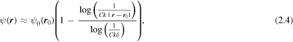
where, in terms of the Euler constant $\gamma =0.57722,$

$$\begin{eqnarray}&&C=\frac{\exp (\gamma )}{2}=0.890536.\end{eqnarray} \tag{ 2.5 }$$

This is the asymptotic form of $\psi$ close to the pinprick, and our main result, illustrated in figure 1.

Far from ${{\boldsymbol{r}}}_{0},$ i.e. away from the pinprick, the Bessel function ${Y}_{0}\left(k\left|{\boldsymbol{r}}{\boldsymbol{-}}{{\boldsymbol{r}}}_{0}\right|\right)$ in (2.3) oscillates, indicating persistent undulations decorating the ambient wave. In the next section we will see that for small $\delta$ this influence is weak; we also describe a slight generalisation.

3.1. Plane wave

For an ambient plane wave in the $x$ direction, with wavelength $\lambda =1,$ punctured at the origin, i.e.

$$\begin{eqnarray}&&{\psi }_{0}\left({\boldsymbol{r}}\right)=\exp \left(2\pi {\rm{i}}x\right),{{\boldsymbol{r}}}_{0}=(0,0),\end{eqnarray} \tag{ 3.1 }$$

the pinpricked wave (2.3) is

$$\begin{eqnarray}&&\psi \left({\boldsymbol{r}}\right)=\exp \left(2\pi {\rm{i}}x\right)-\displaystyle \frac{{Y}_{0}\left(2\pi r\right)}{{Y}_{0}\left(2\pi \delta \right)}.\end{eqnarray} \tag{ 3.2 }$$

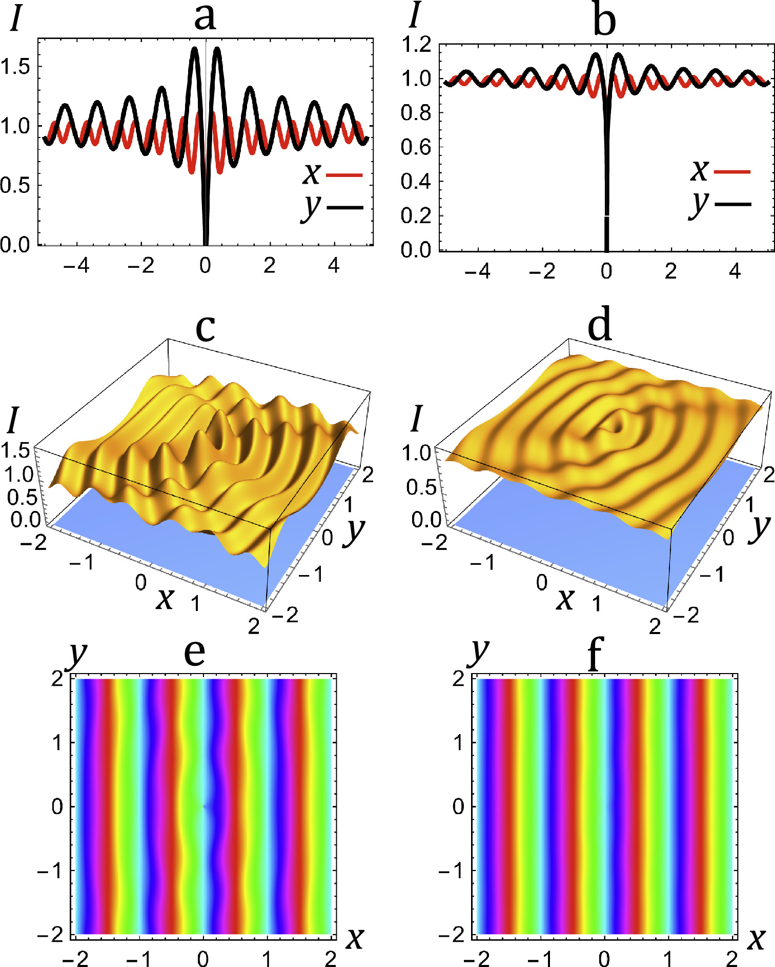
Figure 2 shows the intensity

$$\begin{eqnarray}&&I\left({\boldsymbol{r}}\right)\equiv {\left|\psi \left({\boldsymbol{r}}\right)\right|}^{2}=1-2\cos \left(2\pi x\right)\frac{{Y}_{0}\left(2\pi r\right)}{{Y}_{0}\left(2\pi \delta \right)}+{\left(\frac{{Y}_{0}\left(2\pi r\right)}{{Y}_{0}\left(2\pi \delta \right)}\right)}^{2},\end{eqnarray} \tag{ 3.3 }$$

and the phase $\arg \psi \left({\boldsymbol{r}}\right),$ for two values of $\delta .$ The thinness of the pinprick is evident in (a), (b).

Zoom In Zoom Out Reset image size

Figures 2(a)–(d) show that the distant oscillations are surprisingly persistent even for $\delta ={10}^{-6}\lambda ,$ and slower and stronger in $y$ than $x.$ By contrast, (e), (f) show that the effect on the phase is comparatively weaker, illustrating the fact that pinpricks are not phase singularities (around which the phase would change by a nonzero multiple of $2\pi$).

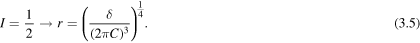
Close to the zero, the limiting form of the intensity is (see 2.4)

$$\begin{eqnarray}&&r\ll 1:I\left({\boldsymbol{r}}\right)\approx 1-\frac{2\mathrm{log}\left(\frac{1}{2\pi {Cr}}\right)}{\mathrm{log}\left(\frac{1}{2\pi C\delta }\right)}.\end{eqnarray} \tag{ 3.4 }$$

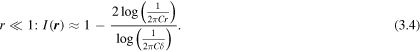
From this it follows that the intensity halfwidth of the pinprick has radius

$$\begin{eqnarray}&&I=\frac{1}{2}\to r={\left(\frac{\delta }{{\left(2\pi C\right)}^{3}}\right)}^{\frac{1}{4}}.\end{eqnarray} \tag{ 3.5 }$$

Far from the pinprick, large-argument Bessel asymptotics (section 10.17(i) of [15]) gives the asymptotic intensity oscillations along the $x$ axis:

$$\begin{eqnarray}&&x\gg 1:I\left(x,0\right)\approx 1-\frac{1+\sqrt{2}\cos \left(4\pi \left|x\right|+\tfrac{\pi }{4}\right)}{\begin{array}{c}{2}^{\tfrac{3}{2}}\mathrm{log}\left(\frac{1}{2\pi C\delta }\right)\sqrt{\left|x\right|}\\ \,\end{array}},\end{eqnarray} \tag{ 3.6 }$$

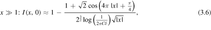
and along the $y$ axis:

$$\begin{eqnarray}&&x\gg 1:I\left(0,y\right)\approx 1-\frac{\cos \left(2\pi \left|y\right|+\tfrac{\pi }{4}\right)}{\begin{array}{c}\mathrm{log}\left(\frac{1}{2\pi C\delta }\right)\sqrt{\left|y\right|}\\ \,\end{array}}.\end{eqnarray} \tag{ 3.7 }$$

These agree to visual accuracy with the exact oscillations in figures 2(a) and (b) (comparison not shown).

For simplicity, an important aspect of the oscillations was not mentioned until now. In the pinprick formula (2.3), the replacement

$$\begin{eqnarray}&&\frac{{Y}_{0}\left(k\left|{\boldsymbol{r}}{\boldsymbol{-}}{{\boldsymbol{r}}}_{0}\right|\right)}{{Y}_{0}\left(k\delta \right)}\to \frac{{Y}_{0}\left(k\left|{\boldsymbol{r}}{\boldsymbol{-}}{{\boldsymbol{r}}}_{0}\right|\right)-{ia}{J}_{0}\left(k\left|{\boldsymbol{r}}{\boldsymbol{-}}{{\boldsymbol{r}}}_{0}\right|\right)}{{Y}_{0}\left(k\delta \right)-{ia}{J}_{0}\left(k\delta \right)}\end{eqnarray} \tag{ 3.8 }$$

leaves the small $\delta$ behaviour close to the pinprick unchanged, but alters the oscillations. For the particular choice $a=1,$ the factor is

$$\begin{eqnarray}&&\frac{{H}_{0}^{\left(1\right)}\left(k\left|{\boldsymbol{r}}{\boldsymbol{-}}{{\boldsymbol{r}}}_{0}\right|\right)}{{H}_{0}^{\left(1\right)}\left(k\delta \right)},\end{eqnarray} \tag{ 3.9 }$$

involving the Bessel function of the third kind. This choice corresponds to the oscillations representing outgoing radiation. In the appendix we will return to this generalisation.

3.2. Circular billiard

Consider azimuthally symmetric waves $\psi \left(r\right)$ in the unit disk with Dirichlet boundary conditions, $\delta$-punctured at the centre $r=0.$ The ambient modes, nonvanishing at $r=0$ and vanishing at $r=1,$ are the zero-order Bessel functions with zeros ${j}_{0,n},$ where $n=\mathrm{1,2,3}\cdots :$

$$\begin{eqnarray}&&{\psi }_{n0}\left(r\right)={J}_{0}\left({j}_{0,n}r\right).\end{eqnarray} \tag{ 3.10 }$$

The punctured modes in the annulus $0\leqslant \delta \leqslant 1,$ with perturbed eigenvalues ${k}_{n}\left(\delta \right),$ exactly satisfying (2.1) with the boundary condition (2.2), are

$$\begin{eqnarray}&&{\psi }_{n}\left(r,\delta \right)={J}_{0}\left({k}_{n}\left(\delta \right)r\right)-\displaystyle \frac{{J}_{0}\left({k}_{n}\left(\delta \right)\delta \right)}{{Y}_{0}\left({k}_{n}\left(\delta \right)\delta \right)}{Y}_{0}\left({k}_{n}\left(\delta \right)r\right)\end{eqnarray} \tag{ 3.11 }$$

(in this case (2.3) is exact.) The eigenvalues ${k}_{n}^{2}$ of the operator in (2.1), with the stated Dirichlet boundary condition at $r=1,$ are determined by

$$\begin{eqnarray}&&\frac{{J}_{0}\left({k}_{n}\left(\delta \right)\right)}{{Y}_{0}\left({k}_{n}\left(\delta \right)\right)}=\frac{{J}_{0}\left({k}_{n}\left(\delta \right)\delta \right)}{{Y}_{0}\left({k}_{n}\left(\delta \right)\delta \right)}.\end{eqnarray} \tag{ 3.12 }$$

Figures 3 and 4 show the punctured modes for $n=1$ and $n=3.$ The pinpricks are clearly visible in figures 3(d) and 4(d), even for $\delta ={10}^{-6}.$ Away from the pinpricks, the modes are visibly altered for $\delta =1/20,$ and hardly so for $\delta ={10}^{-6}.$

Zoom In Zoom Out Reset image size

Zoom In Zoom Out Reset image size

The shift in the eigenvalues, ${\rm{\Delta }}{k}_{n}\left(\delta \right),$ can be easily calculated numerically, or perturbatively from (3.12):

$$\begin{eqnarray}&&\psi \left(1,\delta \right)=0\to {k}_{n}\left(\delta \right)={j}_{0,n}+{\rm{\Delta }}{k}_{n}\left(\delta \right),\end{eqnarray} \tag{ 3.13 }$$

where, using $\delta \ll \lambda ,$

$$\begin{eqnarray}&&{\rm{\Delta }}{k}_{n}\left(\delta \right)=\frac{\pi {Y}_{0}\left({j}_{0,n}\right)}{2{J}_{1}\left({j}_{0,n}\right)\mathrm{log}\left(\frac{1}{C{j}_{0,n}\delta }\right)}+\cdots \end{eqnarray} \tag{ 3.14 }$$

Figure 5 shows the fractional eigenvalue shifts as functions of $\delta .$

Zoom In Zoom Out Reset image size

The formula (3.12) can be simplified using the approximation

$$\begin{eqnarray}&&\frac{{Y}_{0}\left({j}_{0,n}\right)}{{J}_{1}\left({j}_{0,n}\right)}\approx 1.\end{eqnarray} \tag{ 3.15 }$$

This is the asymptotics for $n\gg 1,$ but it can be used even for $n=1$ where the ratio is 0.9822; similarly, we can approximate ${j}_{0,n}\approx \left(n-\tfrac{1}{4}\right)\pi$ (accurate to 2% even for $n=1$). Thus the fractional shift of the $\delta -{\rm{punctured}}$ (pinpricked) mode $n$ is

$$\begin{eqnarray}&&n\gg 1:\frac{{\rm{\Delta }}{k}_{n}\left(\delta \right)}{{j}_{0,n}}\approx \frac{1}{2n\mathrm{log}\left(\frac{1}{C\left(n-\tfrac{1}{4}\right)\pi \delta }\right)}.\end{eqnarray} \tag{ 3.16 }$$

The factor $1/n$ shows that the eigenvalue shift for fixed small $\delta$ gets smaller as $n$ increases, as illustrated in figure 5 for $n=1$ and $n=3.$

The foregoing has considered a single pinprick, but it is clear that the plane can be $\delta$ punctured at more than one place. Indeed, a dense peppering of the plane with zeros can be envisaged, which would be invisible in the limit $\delta \to 0.$ How dense? I conjecture that in the limit as $\delta \to 0$ the pinpricks can form a set of fractal dimension $d\lt 1;$ dimension $d=1$ is excluded because this would include Dirichlet conditions along a line, which would certainly not be invisible.

For waves in three-dimensional space, asymptotically invisible pinpricks would form lines, arbitrarily curved, possibly closed, linked or knotted, and arbitrarily numerous. In addition, there can be point zeros, based on excising small spheres of radius $\delta .$ The theory is similar, with ${Y}_{0}\left(k\delta \right)$ replaced by the spherical Bessel function ${y}_{0}\left(k\delta \right)$ [15], so the radius (intensity half-width) of the pinpricks would be ${\mathscr{O}}\left(\delta \right)$ rather than ${\mathscr{O}}\left({\delta }^{\frac{1}{4}}\right)$ as in (3.5). Extension to higher space dimensions $D$ is clear: asymptotically invisible pinpricks can be created, with codimensions ${C}_{D}=2,\cdots ,D.$

Complementary to pinpricks would be positive spikes ('prickles') instead of zeros. To create these is simple: instead of the negative modification (2.3), add 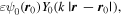$\varepsilon {\psi }_{0}{\left({{\boldsymbol{r}}}_{0}\right)Y}_{0}\left(k\left|{\boldsymbol{r}}{\boldsymbol{-}}{{\boldsymbol{r}}}_{0}\right|\right),$ with $0\lt \varepsilon \ll 1,$ to the ambient wave. As $\varepsilon$ decreases to zero, the prickles get asymptotically invisible.

A note about limits. The emphasis here is the pinprick limit $\delta \to 0.$ Other limits need not commute with it. For example, if the $\delta$-excised disk is in a region of the plane with a rectangular perimeter, or if the plane is compactified into a 2-torus, the system is the Sinai billiard [16], whose geometrical ('classical') trajectories exhibit chaos: exponential separation of infinitesimally close initial trajectories as ${\rm{time}}\,t\to \infty .$ This obviously does not commute with $\delta \to 0,$ because as $\delta$ gets smaller the chaos gets longer to develop, and when $\delta =0$ it never does. And in the wave version, the eigenvalues for finite $\delta$ reflect the classical chaos by exhibiting random-matrix statistics [17–19]. The $\delta \to 0$ limit also does not commute with the classical limit $\hslash \to 0,$ which in this case corresponds to the short-wave limit $\lambda \to 0$ of high excited states: as $\delta$ gets smaller, it is necessary to search higher in the spectrum in order to see the random-matrix statistics (this is discussed in appendix C of [17]).

I thank the Beijing Institute for Mathematical Sciences and Applications (BIMSA) and Peking University for hospitality while this work was carried out. My research was supported by the Leverhulme Trust.

No new data were created or analysed in this study.

Appendix. Corrections to the pinprick formula (2.3)

Here we show how the boundary condition (2.2) can be satisfied exactly. Setting ${{\boldsymbol{r}}}_{0}={\bf{0}}$ and $k=1$ for convenience, we expand the ambient wave in circular-harmonic solutions of (2.1), using polar coordinates:

$$\begin{eqnarray}&&{\psi }_{0}\left({\boldsymbol{r}}\right)=\displaystyle \sum _{n=-{\rm{\infty }}}^{{\rm{\infty }}}{c}_{n}{J}_{n}\left(r\right)\exp \left({in}\phi \right).\end{eqnarray} \tag{ A.1 }$$

(For the example wave (3.1), ${c}_{n}={i}^{n}.$) The approximation (2.3) corresponds to modifying the term $n=0.$

The boundary condition at $r=\delta$ can be satisfied exactly for each $n$ separately, by adding a contribution to ${J}_{n}(r).$ The modification depends on other boundary conditions that the exact $\psi ({\boldsymbol{r}})$ must satisfy. For a real wave, as in section 3.2, the modification is

$$\begin{eqnarray}&&{J}_{n}\left(r\right)\to {J}_{n}\left(r\right)-\frac{{J}_{n}\left(\delta \right)}{{Y}_{n}\left(\delta \right)}{Y}_{n}\left(r\right).\end{eqnarray} \tag{ A.2 }$$

For the infinite plane, the modification can be any combination of incoming and outgoing waves, depending on the radiation condition. For the outgoing choice, it involves Bessel functions of the third kind, as described for $n=0$ at the end of section 3.1, and can be conveniently written

$$\begin{eqnarray}&&{J}_{n}\left(r\right)\to {J}_{n}\left(r\right)-\frac{{J}_{n}\left(\delta \right)}{\left({H}_{n}^{\left(1\right)}\left(\delta \right)\right)}\left({H}_{n}^{\left(1\right)}\left(r\right)\right).\end{eqnarray} \tag{ A.3 }$$

For $\delta \ll 1,$ the difference between the coefficients in (A.2) and (A.3) disappears; the small argument limiting forms of the Bessel functions [15] gives

$$\begin{eqnarray}&&n\ne 0:\frac{{J}_{n}\left(\delta \right)}{{Y}_{n}\left(\delta \right)}\approx \frac{{J}_{n}\left(\delta \right)}{\left({-{iH}}_{n}^{\left(1\right)}\left(\delta \right)\right)}\approx -\frac{\pi \,{\delta }^{2\left|n\right|}\,}{{4}^{n}\left|n\right|{\rm{\Gamma }}{\left(\left|n\right|\right)}^{2}}.\end{eqnarray} \tag{ A.4 }$$

For $\delta \ll 1,$ these $n\ne 0$ coefficients are ${\mathscr{O}}\left({\delta }^{2\left|n\right|}\right)$ and therefore negligible in comparison with the $n=0$ coefficient, which (see (2.4)) is ${\mathscr{O}}\left({\left(\mathrm{log}\left({\delta }^{-1}\right)\right)}^{-1}\right).$ Therefore the $n\ne 0$ corrections correspond to thinner pinpricks, reflecting the familiar s wave scattering of scalar waves by infinitesimal obstacles.

For $n=0,$ the real and outgoing modifications are different for the $r\gg 1$ oscillations. In the example in section 3.1 we have chosen the real modification in equation (3.2), but the order of magnitude of the oscillations is the same for the outgoing case: both vanish as ${\mathscr{O}}\left({\left(\mathrm{log}\left({\delta }^{-1}\right)\right)}^{-1}\right).$