


Abstract
We conducted a simulation of H2SO4 vapor, H2O vapor, and H2SO4–H2O liquid aerosols from 40 to 100 km, using a 1D Venus cloud microphysics model based on the one detailed in Imamura & Hashimoto. The cloud distribution obtained is in good agreement with in situ observations by Pioneer Venus and remote-sensing observations from Venus Express (VEx). Case studies were conducted to investigate sensitivities to atmospheric parameters, including eddy diffusion and temperature profiles. We find that efficient eddy transport is important for determining upper haze population and its microphysical properties. Using the recently updated eddy diffusion coefficient profile by Mahieux et al., our model replicates the observed upper haze distribution. The H2O vapor distribution is highly sensitive to the eddy diffusion coefficient in the 60–70 km region. This indicates that updating the eddy diffusion coefficient is crucial for understanding the H2O vapor transport through the cloud layer. The H2SO4 vapor abundance varies by several orders of magnitude above 85 km, depending on the temperature profile. However, its maximum value aligns well with observational upper limits found by Sandor et al., pointing to potential sources other than H2SO4 aerosols in the upper haze layer that contribute to the SO2 inversion layer. The best-fit eddy diffusion profile is determined to be ∼2 m2 s−1 between 60 and 70 km and ∼360 m2 s−1 above 85 km. Furthermore, the observed increase of H2O vapor concentration above 85 km is reproduced by using the temperature profile from the VEx/SOIR instrument.
Export citation and abstract BibTeX RIS

Original content from this work may be used under the terms of the Creative Commons Attribution 4.0 licence. Any further distribution of this work must maintain attribution to the author(s) and the title of the work, journal citation and DOI.
1. Introduction
Venus is globally shrouded by thick clouds extending from ∼45 to 70 km, which play an essential role in many atmospheric processes, such as radiation, chemistry, and dynamics. Hansen & Hovenier (1974) reported that the cloud particles are composed of a H2SO4–H2O solution. Venera, VEGA, and Pioneer Venus (PV) missions played a crucial role in establishing the basic features composing the Venusian clouds. Nephelometers on board Venera 9, 10, and 11 landers measured the microphysical properties of the clouds and suggested that the particle size distribution is at least bimodal between 48 and 57 km (Marov et al. 1980). The VEGA-1 balloon measured the backscattering of the clouds between 50 and 53 km and suggested that the clouds are highly variable in terms of time and altitude (Sagdeev et al. 1986). Measurement of the clouds' microphysical properties was also conducted by the Cloud Particle Size Spectrometer (LCPS) on board the PV Large probe (Knollenberg & Hunten 1980). The in situ measurements revealed a triple-layered cloud structure: the lower cloud spans from 47 to 51 km, the middle cloud from 51 to 57 km, and the upper cloud from 57 to 70 km; note that these values vary with latitude, as the clouds are found at lower altitudes at the poles. The lower and middle cloud layers exhibit a trimodal size distribution with peak radii at ∼0.15 μm (Mode 1), ∼1.2 μm (Mode 2), and ∼3.5 μm (Mode 3). The formation of these two layers is driven by condensation of H2SO4-rich air supplied from the subcloud region. By contrast, the upper cloud layer exhibits a bimodal distribution with peak radii at ∼0.2 μm (Mode 1) and ∼1.0 μm (Mode 2). Particles in the upper cloud layer are formed by photochemical production of H2SO4 vapor occurring between 60 and 70 km (Winick & Stewert 1980; Yung & Demore 1982; Krasnopolsky 2012; Zhang et al. 2012), and the H2SO4 found below the cloud deck is regarded as the direct result of the upper cloud particle sedimentation. Furthermore, observations by Venus Express (VEx) have provided valuable insights, enhancing our understanding of the cloud structure on Venus. Markiewicz et al. (2018) retrieved the average upper cloud radius of 1.0–1.2 μm from glory observations by the Venus Monitoring Camera (VMC). Cottini et al. (2012) obtained a mass percentage of sulfuric acid inside the upper cloud droplets of 75%–83%, using the Visible and Infrared Thermal Imaging Spectrometer (VIRTIS). Oschlisniok et al. (2021) retrieved H2SO4 concentration below the cloud bottom altitude, ranging between 12 ppm at the equator and ∼6 ppm at the midlatitude, using data obtained from Venus Express radio science experiment (VeRa). For more comprehensive insights into the cloud structure and droplet size distribution, the review by Titov et al. (2018) is recommended, particularly Table 1 of their article.
Table 1. Recent Numerical Models That Include Cloud Processes
| Model | Dimension | Microphysics | Dynamics | Chemistry | Altitude Range |
|---|---|---|---|---|---|
| Ando et al. (2020) | 3D | ⋯ | Diffusion and advection | H2O–H2SO4 system a | 0–120 km |
| Dai et al. (2022) | 1D | ⋯ | Eddy diffusion | H2O–H2SO4 system | 40–80 km |
| Määttänen et al. (2023) | 0D | Modal | ⋯ | H2O–H2SO4 system | ⋯ |
| McGouldrick & Barth (2023) | 1D | Sectional | Eddy diffusion | H2O–H2SO4 system | 40–80 km |
| Stolzenbach et al. (2023) | 3D | ⋯ | Diffusion and advection | Photochemistry including 31 gas species | 0–95 km |
| Karyu et al. (2023) | 3D | ⋯ | Diffusion and advection | Sulfur cycle including SO2, SO3, H2SO4, H2O, CO2, CO, and O b | 0–95 km |
| This study | 1D | Sectional | Eddy diffusion | H2O–H2SO4 system | 40–100 km |
Notes.
a The H2SO4 production is parameterized as a function of solar zenith angle. b The O density is fixed as a function of solar zenith angle.Download table as: ASCIITypeset image
Particles have been observed in the region above the cloud top, between 70 and 110 km, commonly referred to as the upper haze layer. Kawabata et al. (1980) characterized this layer using polarization data obtained by Cloud PhotoPolarimeter (CPP) on board PV, reporting an effective radius of the haze particles of ∼0.23 μm. More recent observations by Spectroscopy for Investigation of Characteristics of the Atmosphere of Venus (SPICAV) on board VEx further corroborate the presence of the upper haze layer. Using the solar occultation data obtained by the Solar Occultation at Infrared (SOIR) instrument and SPICAV-UV, Wilquet et al. (2009) determined that the upper haze consists of two particle modes with distinct radii. Mode 1 particles have a mean radius ranging from 0.1 to 0.3 μm, while Mode 2 particles have a mean radius between 0.4 and 1.0 μm. A follow-up study by Wilquet et al. (2012) revealed that the vertical profiles of aerosol extinction coefficient at 3 μm vary significantly across both latitude and time. Luginin et al. (2016) observed the upper haze layer using the data set obtained by SPICAV-IR and obtained a mean radius of ∼0.5 μm when a unimodal distribution was assumed. A follow-up study by Luginin et al. (2024) reported that bimodal distribution is observed in more than 50% of retrieved profiles in the upper haze layer. Takagi et al. (2019) showed that haze particles are ubiquitous above 90 km using the SOIR data.
The upper haze layer is thought to participate in the sulfur chemical cycle within the mesosphere between 70 and 100 km. Previous ground-based measurements using the JCMT facilities by Sandor et al. (2010) reported that the SO2 volume mixing ratio (VMR) is about an order of magnitude higher than that predicted by photochemical models, proposing that sulfate aerosols could account for such elevated levels of SO2. Using the data set collected by SOIR on board VEx, Belyaev et al. (2012) and the updated study by Mahieux et al. (2023a), which could reconcile the SOIR/VEx and JCMT observations, revealed that the SO2 VMR is higher between 85 and 105 km than it is between 75 and 85 km. This peculiar SO2 profile is commonly referred to as the inversion layer. A 1D photochemical model study by Zhang et al. (2010) showed that the observed inversion layer could be accounted for by the photolysis of H2SO4 vapor, which originates from the evaporation of the upper haze. In their model, they assumed a fixed H2O VMR of 0.5 ppm and a saturation H2SO4 VMR as high as ∼1 ppm based on the nighttime temperature profile obtained by SOIR. Krasnopolsky (2012) pointed out that the nighttime temperature assumed by Zhang et al. (2010) cannot be applicable to the H2SO4 photolysis that occurs on the dayside. Later, Sandor et al. (2012) used ground-based observations to measure mesospheric H2SO4 abundance and found that the upper limit of H2SO4 VMR was ∼3 ppb. This is orders of magnitude lower than the H2SO4 VMR assumed by Zhang et al. (2010). The role of the upper haze layer as a source of sulfur species remains a topic of debate.
In the Venusian atmosphere, the H2O VMR decreases more than one order of magnitude from ∼30 ppm below the clouds to ∼1 ppm above them. It is important to investigate the H2O budget in the cloud and haze layers because the H2O vapor abundance below the homopause regulates the escape rate of hydrogen (Catling & Kasting 2017) and thus the planet's water history. The previous near-infrared observations reported that the H2O VMR is ∼30 ppm below 40 km (Marcq et al. 2008; Bézard et al. 2011; Chamberlain et al. 2013; Arney et al. 2014; Fedorova et al. 2015). On the other hand, recent observations by VEx reported a H2O VMR of 0.5–3 ppm near and above the cloud-top altitude (Fedorova et al. 2008; Cottini et al. 2015; Chamberlain et al. 2020; Mahieux et al. 2023b). The H2SO4 droplets strongly absorb H2O vapor through the hygroscopic effect. This phenomenon leads to the Venus cloud-top conditions similar to Earth's stratosphere, which exhibits extremely low H2O abundance (McGouldrick et al. 2011). In addition to the hygroscopic effect, chemical reactions involving gaseous H2O and SO2 also play an important role in controlling the H2O VMR in the upper cloud layer (e.g., Winick & Stewert 1980; Yung & Demore 1982; Krasnopolsky 2012; Shao et al. 2020). Overall, the H2O VMR in the mesosphere is determined by a delicate balance among the hygroscopic effect, chemical net loss, and transport processes.
Cloud microphysics models are a powerful tool to investigate the Venusian cloud system and condensational gas cycles. Imamura & Hashimoto (2001) developed such a model including a simple chemical reaction system involving H2O and H2SO4. They showed that the dynamical mixing is essential for reproducing the observed trimodal size distribution. The Community Aerosol and Radiation Model for Atmospheres (CARMA) has been commonly used for the study of the cloud microphysical properties (McGouldrick & Toon 2007; Gao et al. 2014; Parkinson et al. 2015; McGouldrick 2017; McGouldrick & Barth 2023). Gao et al. (2014) investigated the size evolution of cloud and haze particles using CARMA extending from 40 to 100 km to simulate the upper haze layer. They showed that the upper haze exhibits a unimodal distribution at a steady state, but a bimodal structure can be induced by transient upward winds in the mesosphere. Using the same model, Parkinson et al. (2015) explored how cloud structure varies with latitudinal and local time temperature patterns. They confirmed that the steady-state distribution is unimodal in the upper haze layer across all locations. Recently, McGouldrick & Barth (2023) simulated the cloud structure and distribution of gaseous H2SO4 and H2O using CARMA in the 40–80 km region. They showed that the physical characteristics of condensation nuclei (CN) can induce long-term cloud variations. However, studies led by Gao et al. (2014) and Parkinson et al. (2015) maintained a fixed H2O VMR, while those led by Imamura & Hashimoto (2001) and McGouldrick & Barth (2023) calculated a H2O VMR profile but suggested a higher H2O VMR above the upper cloud region compared to the VEx observations. Moreover, to the best of our knowledge, no studies have simultaneously simulated the microphysical properties of aerosol and distributions of condensational gas species including H2O up to 100 km. Table 1 summarizes recent advancements in Venus cloud modeling.
In this study, we investigated the distributions of H2SO4–H2O aerosols, H2SO4 vapor, and H2O vapor from 40 up to 100 km using a 1D cloud microphysics model. In Section 2, we describe the model and settings for case studies in which we varied both the eddy diffusion and temperature profiles. In Section 3, we show the simulation results including all case studies. In Section 4, we discuss the implications drawn from the simulation results and the atmospheric processes related to the Venusian clouds. Finally, we provide a summary of the present study in Section 5.
2. Model Description
2.1. Overview
The model equations used in this study are based on a 1D cloud microphysics model developed by Imamura & Hashimoto (2001). We note, however, that the purpose of using a 1D model is different from Imamura & Hashimoto (2001), who reproduced the equatorial atmosphere by incorporating the upward branch of the Hadley circulation into the 1D model. Here we focus on the globally averaged vertical structure by representing all vertical transport processes, including large-scale advection such as the Hadley circulation, by eddy diffusion, and thus the advection by vertical winds is absent in the equations. The model simulates dynamical and cloud microphysical processes in a 1D column of CO2 air from 40 to 100 km. As a major update from the previous work by Imamura & Hashimoto (2001), we extended the model top altitude from 70 to 100 km to include the upper haze layer. CN and cloud droplets are modeled with discrete size bins. The size bins are divided into 23 bins between 0.17 and ∼30 μm, in which the volume doubles from one bin to the next. The smallest size bin represents Mode 1 particles, which are assumed to be insoluble CN. Size bins larger than the smallest bin represent droplets, whose liquid composition consists of a binary solution of H2SO4 and H2O. The cloud size distribution is a function of the particle mass m, the altitude z, and the time t. It is calculated based on the 1D continuity equation defined without the advection term (modified after Imamura & Hashimoto 2001):
where C(m, z, t) is the cloud particle number density, ρ(z) is the atmospheric density, Kzz
(z) is the vertical eddy diffusion coefficient of air, wsed(m, z) is the sedimentation velocity of cloud particles, G(m, z, t) is the condensational growth rate,  is the coagulation kernel between cloud particles with mass m and
  , and mcn and mmax are the masses of condensational nucleus and particle with maximum size, respectively. The first term on the right-hand side is vertical transport by eddy diffusion. The second term accounts for vertical transport due to particle sedimentation. The third term represents the growth through condensation, and the fourth and fifth terms represent particle size evolution resulting from coagulation.
Brownian diffusion is accounted for in the coagulation process. The CN is treated the same way as in the earlier work (Imamura & Hashimoto 2001). Particles in the smallest size bin act as the CNs. The composition and microphysical properties of CNs are unknown. Therefore, for simplicity, we assume that they do not coagulate with each other. Thermal equilibrium is assumed when calculating the H2SO4 mass fraction in the cloud droplets, considering that equilibrium adjustment is achieved by the exchange of H2O molecules between the droplet surface and the surrounding environment.
Regarding the sedimentation process, while the previous work by Imamura & Hashimoto (2001) used the Stokes velocity, we implemented the Cunningham slip-flow correction as follows (Jacobson 2005):
where r(m) is the particle radius corresponding to the mass m; ρp is the density of the particle; g = 8.7 m s−2 is the gravitational acceleration; η = 1.5 × 10⁻⁵ kg m−1 s−1 is the viscosity of CO2 gas; A, B, and C are experimental parameters set to be 1.249, 0.42, and 0.87, respectively, following Kasten (1962); and Kn(z) is the Knudsen number for air. The inclusion of the Cunningham slip-flow correction is crucial for accurately estimating sedimentation velocity in thin air owing to strong dependency of Kn on altitude. This effect, which was not included in earlier work by Imamura & Hashimoto (2001), has limited impact on particle size distribution between 40 and 70 km.
We also consider the chemical production of H2SO4 vapor and loss of H2O vapor through the following net reaction, as included in previous works (Imamura & Hashimoto 2001; McGouldrick 2017; McGouldrick & Barth 2023):

It demonstrates that the production of one H2SO4 molecule results in the loss of one H2O molecule. We updated the production rate of H2SO4 using the photochemical model results from Krasnopolsky (2012). The updated production rate is a globally averaged value, consistent with the other settings in the present study. The column integrated production rate is about 5.7 × 10¹⁵ m−2 s−1, which is approximately half of the rate used in the study by Imamura & Hashimoto (2001). In addition, the peak altitude of the production rate is located at ∼66 km following Krasnopolsky (2012), while it was situated at 61 km in the previous work. We also adopted the CN production rate introduced by Imamura & Hashimoto (2001), who assumed that the CNs are made of elemental sulfur produced by reaction (3) and have the same radius as particles in Mode 1. The production rate of CN, Pcn, is expressed as

where P1(z) is the H2SO4 vapor production rate, rcn and  are respectively the radius and mass density of CN, and Ms
is the molecular mass of elemental sulfur. The photochemical production rate profiles of H2SO4 vapor and the CN are shown in Figure 1. It should be noted that if the production rate of CNs matches that of reaction (3), it implies the unavailability of elemental sulfur for the chemistry of this cycle. This is a simplistic assumption and is not corroborated by current findings on the net sulfur production from photochemical models. These models also fail to account for the potential loss of sulfur into droplets, where sulfur primarily reacts with O2. However, studying the interaction between the sulfur chemical cycle and CN production goes beyond the scope of this paper.
are respectively the radius and mass density of CN, and Ms
is the molecular mass of elemental sulfur. The photochemical production rate profiles of H2SO4 vapor and the CN are shown in Figure 1. It should be noted that if the production rate of CNs matches that of reaction (3), it implies the unavailability of elemental sulfur for the chemistry of this cycle. This is a simplistic assumption and is not corroborated by current findings on the net sulfur production from photochemical models. These models also fail to account for the potential loss of sulfur into droplets, where sulfur primarily reacts with O2. However, studying the interaction between the sulfur chemical cycle and CN production goes beyond the scope of this paper.
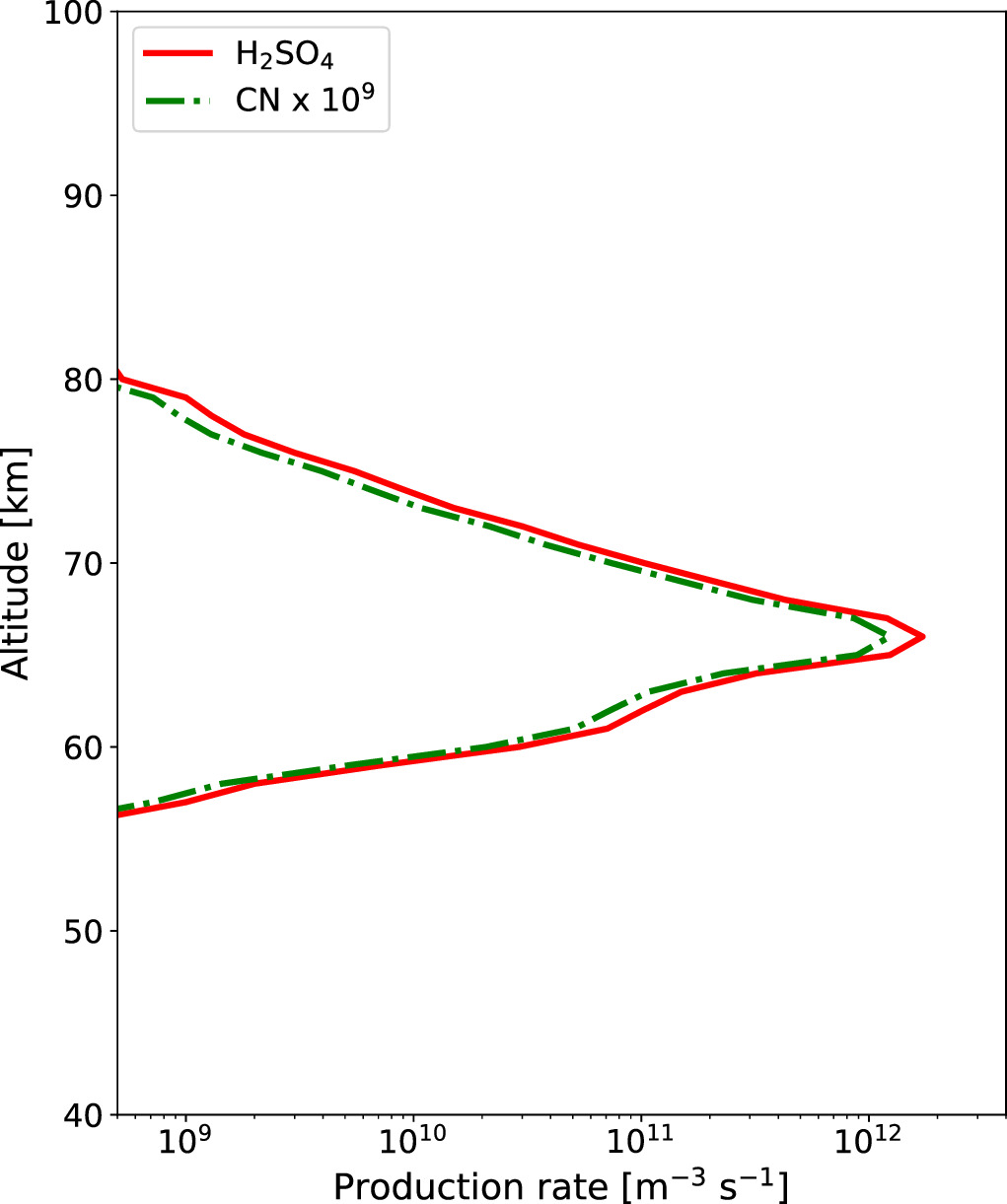
Figure 1. Vertical profiles of H2SO4 vapor (red solid line) and CN (green dashed–dotted line) production rates used in the model. The H2SO4 vapor production rate is adapted from Krasnopolsky (2012).
Download figure:
Standard image High-resolution imageSelecting only one CN size bin may overlook the impact of CNs on microphysical processes. Knollenberg & Hunten (1980) found a wide size distribution of CNs that includes significant numbers of particles both larger and smaller than 0.17 μm. Larger CNs might represent a nonnegligible sink of H2SO4 and H2O, while smaller CNs might be less relevant owing to the Kelvin effect, which hinders condensation on smaller particles. Moreover, it is improbable that CNs with radii as large as 0.17 μm originate directly from photochemical processes because the initial CN products are considerably smaller and contain far fewer molecules. These particles grow to sizes around 0.17 μm through nucleation and coagulation over time, leading to a broad size distribution. Thus, the simplified treatment of CNs in the present study may overestimate the number of photochemically produced CNs as large as 0.17 μm. These effects should be investigated by incorporating a CN size distribution in a future study.
As mentioned earlier, the detailed settings for cloud microphysical processes and underlying chemistry are also adapted from Imamura & Hashimoto (2001); we refer the reader to this paper for more details. In the following subsections, we outline the parameters used in case studies and describe the calculation settings.
2.2. Eddy Diffusion Profile
The nominal eddy diffusion profile is established based on the past estimations (see Figure 2). Eddy diffusion is not an observable quantity. It is rather a conceptual parameterization of atmospheric dynamics over a variety of scales.

Figure 2. Vertical profiles of eddy diffusion coefficient (Kzz ) for the Nominal Case (black solid line), Case 1 (red dotted line), Case 2 (blue double-dotted–dashed line), and Case 3 (green dashed–dotted line), with estimated values by von Zahn et al. (1980), Woo et al. (1982), Mahieux et al. (2021), and Woo & Ishimaru (1981) labeled as vZ1980, W1982, M2021, and WI1981, respectively. The arrow of WI1981 indicates that the value is the upper limit.
Download figure:
Standard image High-resolution imageIn detailing the historical perspective, radio scintillation measurements have played an important role. They estimated the contribution of small-scale turbulence to the diffusion coefficient, approximating it to be ∼0.2 m2 s−1 at 45 km (Woo et al. 1982) and ∼4 m2 s−1 at 60 km (Woo & Ishimaru 1981). To align our estimated eddy diffusion profile with these observations, we interpolate the eddy diffusion coefficient from 0.1 m2 s−1 at the bottom boundary (40 km) to 4 m2 s−1 at 60 km. Consequently, the interpolated eddy diffusion is ∼0.2 m2 s−1 at 45 km, consistent with the aforementioned studies.
For a more nuanced representation, we considered the influence of convective mixing in the cloud due to infrared heating of the cloud base. This phenomenon, evidenced by the neutral static stability observed by entry probes (e.g., Seiff et al. 1980) and the results from PV, VEx, and Akatsuki radio occultation (Kliore & Patel 1982; Tellmann et al. 2009; Imamura et al. 2017), necessitated an adjustment in our model. Following the work by Imamura & Hashimoto (2001), we incorporated an enhanced eddy diffusion coefficient of 250 m2 s−1 centered at 53 km.
It is important to note the theoretical insights from Baker et al. (1998, 1999, 2000a, 2000b), which indicated that downwelling plumes within the convective layer may extend into the subcloud region, potentially inducing substantial vertical mixing. This convective mixing process can alter the size distribution of particles, as reported in the studies by Imamura & Hashimoto (2001) and McGouldrick & Toon (2007). While this effect is not extensively examined in the current study, its possible impacts on cloud microphysics will be addressed in Section 3.1.
Between 60 and 70 km, the eddy diffusion profile is held constant at the 60 km value for the convenience of parameter studies. The eddy diffusion above 85 km is determined based on past estimations by von Zahn et al. (1980). The eddy diffusion coefficient was derived by comparing observed gas species profiles with those calculated numerically using a 1D diffusion equation. The formulated coefficient was ∼1.4 × 10⁹[M]−0.5 m2 s−1, yielding a value of ∼10 m2 s−1 at 90 km. Thus, we use this value as a typical eddy diffusion coefficient above 85 km. For the layer between 70 and 85 km, the eddy diffusion coefficient is deduced by interpolating the values obtained for the adjacent layers, providing a consistent and gradual transition in the profile.
To investigate the effects of eddy transport processes on particles and gas species, we performed a case study that consisted of four pairs of different eddy diffusion coefficients at 60–70 km and 85–100 km (Cases 1, 2, and 3, in addition to the Nominal Case; see Figure 2). The estimation of eddy diffusion using radio scintillation is based on the assumption that all observed signal fluctuations result from small-scale refractive index structures caused by turbulence; however, the refractive index fluctuation can be due to gravity waves rather than turbulence (Leroy & Ingersoll 1996). Consequently, the eddy diffusion coefficient derived by Woo & Ishimaru (1981) is likely an upper limit. On the other hand, larger-scale eddies, including the mean meridional circulation, can also contribute to vertical transport, and their contributions should be included in the eddy diffusion coefficient in the 1D model. To explore this variability and its impact on particle and gas-phase species distributions, we reduced the eddy diffusion coefficient by a factor of 2 between 60 and 70 km for Cases 2 and 3. Recently, Mahieux et al. (2021) estimated the eddy diffusion coefficient in the mesosphere using a 1D photochemical model and CO and CO2 profiles obtained by the SOIR instrument on board VEx and He and CO2 observations by PV. They derived a coefficient of ∼360 m2 s−1 from 80 to 100 km, an order of magnitude larger than the value obtained by von Zahn et al. (1980). Although Mahieux et al. (2021) derived a complete data set of the eddy diffusion coefficient ranging from 80 to 130 km, the bottom boundary in their 1D photochemical model was 85 km. Therefore, we use the value of 360 m2 s−1 above 85 km for the parameter study (Cases 1 and 3). These four eddy diffusion cases are determined as four patterns composed of pairs of eddy diffusion coefficients for the 60–70 km and 80–100 km altitude ranges, with interpolation between the coefficients for these two ranges.
2.3. Background Atmosphere
The background temperature and pressure profiles are taken from the Venus International Reference Atmosphere (VIRA; Seiff et al. 1985) for the Nominal Case and eddy diffusion case studies. We chose the midlatitude profiles to represent the global average of the background atmosphere, as shown in Figure 3. The temperature and pressure profiles are held constant in the calculation.

Figure 3. (a) Vertical profiles of temperature used in the model. The black solid line represents the temperature profile adapted from Seiff et al. (1985) and is used for the Nominal Case, as well as for Cases 1, 2, and 3. The magenta dashed line represents the temperature profile above 85 km adapted from Mahieux et al. (2015) and is used for Cases 4 and 5. (b) Vertical profile of pressure (Seiff et al. 1985) used in the model.
Download figure:
Standard image High-resolution imageIn addition, we defined case studies using a different temperature profile obtained by the VEx observations. Bertaux et al. (2007) found a warm layer in the Venus mesosphere using the SOIR data set, indicating that the temperature above 85 km could be up to 50 K higher than previously reported. Subsequent studies also confirmed the existence of this warm layer during the course of VEx observations (Mahieux et al. 2012, 2015, 2023b). Mahieux et al. (2023b) proposed that the observed significant temperature differences between the VIRA and SOIR data can be attributed to the variations in temperature distribution with respect to local time, since SOIR observations were all confined to the terminator region. The uncertainties on the individual SOIR temperature profiles vary between 20 and 40 K, while the variability is around 50 K at all altitudes. The temperature difference between the VIRA and SOIR measurements could affect particle and gas distributions by changing the saturation vapor pressure. Therefore, we considered the midlatitude temperature profile from Mahieux et al. (2015) to test the sensitivity toward temperature (Figure 3) in Cases 4 and 5. The SOIR temperature profiles are limited to altitudes above 80 km. We integrated these profiles with those from VIRA to establish a comprehensive temperature distribution for all the altitudes of interest in our model. This integration was achieved by seamlessly connecting the SOIR data with the distributions from VIRA. The connection point was carefully chosen at the altitude where the temperature distributions from VIRA and SOIR naturally intersect, ensuring a continuous temperature profile across the entire altitude range under study. We use the same eddy diffusion coefficient for the Nominal Case as for Case 4 as a control experiment with the SOIR temperature profile. On the other hand, Case 5 uses the same eddy diffusion coefficient as in Case 3, as it well replicates the observed particle and gas distributions. The names of each case (Nominal, Case 1, Case 2, Case 3, Case 4, and Case 5), along with their corresponding parameters, are listed in Table 2. It is important to note that the SOIR temperature profiles exhibit large interprofile variability. This variation can impact condensation and evaporation processes, potentially resulting in changes to aerosol size and acidity. However, the study of the microphysical response to such variation is beyond the scope of our current research.
Table 2. List of Case Studies and the Corresponding Eddy Diffusion and Temperature Profiles
| Case Name | Eddy Diffusion Coefficient at 60–70 km (m2 s−1) | Eddy Diffusion Coefficient at 85–100 km (m2 s−1) | Temperature Profile |
|---|---|---|---|
| Nominal | 4 (a) | 10 (b) | VIRA (d) |
| Case 1 | 4 (a) | 360 (c) | VIRA (d) |
| Case 2 | 2 | 10 (b) | VIRA (d) |
| Case 3 | 2 | 360 (c) | VIRA (d) |
| Case 4 | 4 (a) | 10 (b) | VEx/SOIR (e) |
| Case 5 | 2 | 360 (c) | VEx/SOIR (e) |
References. (a) Woo & Ishimaru (1981); (b) von Zahn et al. (1980); (c) Mahieux et al. (2021); (d) Seiff et al. (1985); (e) Mahieux et al. (2015).
Download table as: ASCIITypeset image
2.4. Boundary and Initial Conditions
Table 3 shows the initial and boundary conditions in our simulations, which are determined based on past observations. The H2O vapor VMR is reported to be ∼30 ppm below 40 km (Marcq et al. 2008; Bézard et al. 2011; Chamberlain et al. 2013; Arney et al. 2014; Fedorova et al. 2015). We take this value as the bottom boundary condition for the H2O vapor. The bottom boundary for the H2SO4 vapor VMR is set at 4 ppm, based on previous observations from both Magellan (Kolodner & Steffes 1998) and VEx (Oschlisniok et al. 2021). The in situ observations reported by Knollenberg & Hunten (1980) suggested that the Mode 1 particles extended below the cloud layer. These particles are assumed to be nonvolatile since H2SO4 vapor cannot exist in the liquid phase within the subcloud region. Therefore, the particle number density for the smallest radius is set at 4 × 10⁷ m−3, based on the number density of the Mode 1 particles from in situ observations. The mixing ratio gradients of cloud particles, H2SO4 vapor, and H2O vapor are set to be zero at the top boundary. The initial conditions for H2O, H2SO4 VMR, and the smallest radius bin are set to match the bottom boundary values across all vertical levels. The aerosol and gas species profiles reach a steady state within ∼50 Venusian years (11,250 Earth days) starting from these initial conditions. This timescale is much longer than the timescales of the physical processes incorporated within the model, such as eddy diffusion, sedimentation, condensation, and coagulation. We performed the simulation for 100 Venusian years (22,500 Earth days) and present the steady-state results in the next section.
Table 3. Boundary Conditions
| Altitude | CN Number Density | Droplet Number Density | H2SO4 VMR | H2O VMR |
|---|---|---|---|---|
| 40 km (bottom) | 4 × 10⁷ m−3 | 0 m−3 | 4 ppm | 30 ppm |
| 100 km (top) |

|

|

|

|
Note. The mixing ratio is expressed as f.
Download table as: ASCIITypeset image
3. Model Results
3.1. Sensitivity to Eddy Diffusion Profiles
Figures 4 and 5 show the simulated size distribution in the Nominal Case and Case 1. The particle size distribution can be divided into three regions by its formation processes, being consistent with the previous microphysics studies (e.g., Gao et al. 2014; McGouldrick & Barth 2023): the lower and middle cloud (47–57 km), the upper cloud (57–70 km), and the upper haze (70–100 km) regions. The upper cloud particles are formed through the condensation of photochemically produced H2SO4 vapor onto CN, which are also produced photochemically through reaction (3) within the same altitude range. The calculated mode radius for the upper cloud layer is ∼0.7 μm, which corresponds to Mode 2 particles but is somewhat underestimated. The lower and middle clouds exhibit a bimodal size distribution, with peaks at the smallest radius bin (0.17 μm) and ∼3 μm corresponding to Modes 1 and 3, respectively (Figures 5(a) and (c)). Between 51 and 53 km, the Kelvin effect inhibits the condensational growth of submicron particles, allowing larger particles to grow. The evaporation of the submicron particles and the upward diffusion transport of CN from the bottom boundary contribute to the formation of the peak at the smallest bin of 0.17 μm. Conversely, the larger peak forms as a result of condensational growth of the photochemically produced particles descending from the upper cloud region. The condensation process is driven by H2SO4-rich air ascending from lower altitudes in the convective layer, where strong eddy diffusion is assumed (see Figure 2).
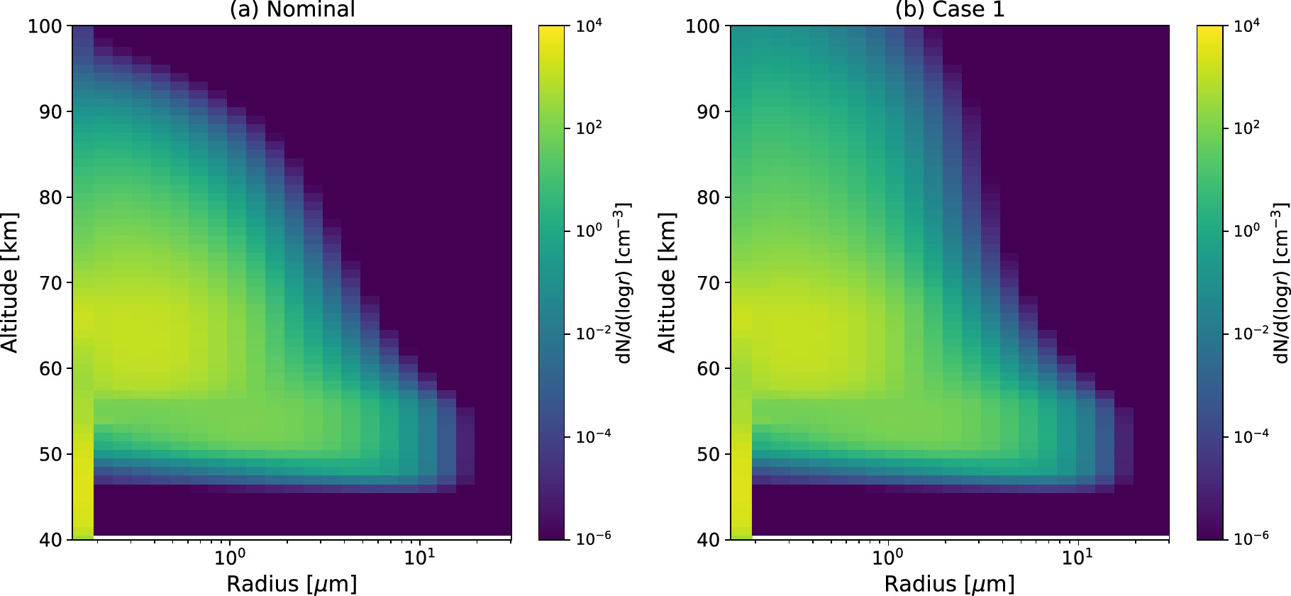
Figure 4. The simulated particle size distribution as a function of radius and altitude in (a) the Nominal Case and (b) Case 1.
Download figure:
Standard image High-resolution image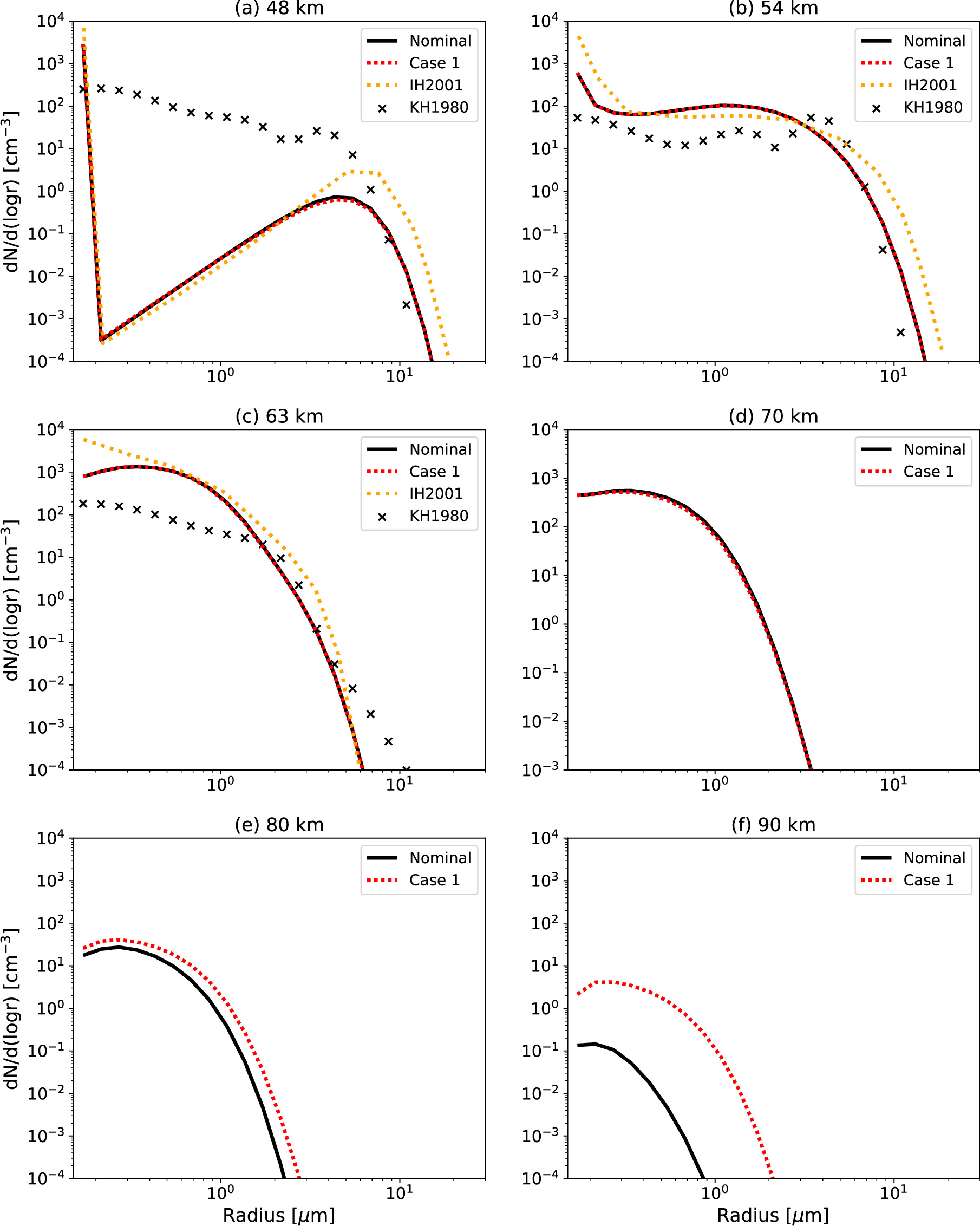
Figure 5. The simulated particle size distribution as a function of radius at (a) 48 km, (b) 54 km, (c) 63 km, (d) 70 km, (e) 80 km, and (f) 90 km in the Nominal Case (black solid line) and Case 1 (red dotted line) in comparison with the previous work by Imamura & Hashimoto (2001; labeled as IH2001). The size distribution measured by the LCPS on board PV (Knollenberg & Hunten 1980) is plotted as KH1980.
Download figure:
Standard image High-resolution imageAbove 53 km, the H2SO4 supersaturation becomes sufficiently high to suppress the Kelvin effect, allowing all particles to undergo condensational growth (Figure 5(b)). Consequently, the smaller peak clearly seen below 53 km altitude eventually merges into the size distribution of the upper cloud. Below 51 km altitude, all particles start to evaporate because of the increasing H2SO4 saturation vapor pressure. The evaporation gradually decreases the droplet number density, leading to the near-complete disappearance of droplets around the cloud base at around 47 km altitude.
Figure 5 demonstrates that the size distribution simulated in the present study closely agrees with earlier work by Imamura & Hashimoto (2001). They showed that the size distribution in the lower and middle cloud layers is bimodal at steady state and that a trimodal distribution can form owing to convective mixing. Furthermore, Baker et al. (1998) suggested that the microphysical properties of the clouds could be altered by condensation processes initiated by cold downwelling plumes from neutrally stable regions in the cloud layers. This implies that the absence of an explicit connection with convective activity in the current study may explain why a trimodal distribution is not observed in these cloud layers.
The upper haze features a broad, unimodal size distribution with a mode radius of ∼0.4 μm (Figures 5(e) and (f)). This radius possibly represents Mode 2 particles as observed by Wilquet et al. (2009) or the effective radius calculated by Luginin et al. (2016), assuming a unimodal size distribution. The particle population in the upper haze is maintained by the upward transport of particles from the upper cloud layer via eddy diffusion.
Changes in the eddy diffusion coefficient above 85 km lead to an enhanced upper haze population. It is evident that the upper haze extends vertically more than in the Nominal Case because of efficient eddy diffusion transport (Figure 4(b)). The size distribution closely resembles that of the Nominal Case at 70 km, but the differences between the two cases become increasingly evident at higher altitudes (Figures 5(d), (e), and (f)). The total particle number density of Case 1 is orders of magnitude larger than in the Nominal Case at 90 km, and larger particles are more abundant in Case 1. This underscores the importance of eddy diffusion transport in shaping the upper haze particle population and its microphysical properties.
Figure 6 shows the simulated cloud structure as a function of altitude. To obtain the mass loading, we calculated the density of the H2SO4–H2O solution droplets by interpolating the density of pure H2O liquid and pure H2SO4 liquid based on weight fraction of H2SO4 (see Figure 9(a)). For the determination of the extinction coefficient, the open-source software MiePython (Prahl 2023) is used to calculate the Mie scattering extinction efficiency of the aerosols. For the input of Mie scattering calculation, we used the refractive index from Palmer & Williams (1975) as a function of the concentration of the H2SO4–H2O solution. The simulated mass loading in the Nominal Case is basically consistent with the PV in situ observations by Knollenberg & Hunten (1980) (Figure 6(a)). The mass loading is highest in the middle cloud layer owing to rapid cloud formation induced by convective activity, aligning with in situ observations. The simulated value is about a factor of 2 smaller than the observed one in the middle cloud layer. The mass loading in the upper cloud is consistent with the observations, although slightly underestimated by a factor of 2. The in situ observations were conducted at the equator, capturing the photochemical production rates of H2SO4 vapor and CN in low latitudes. In contrast, our model uses rates from midlatitudes, which are lower. This likely accounts for the discrepancy between the simulated and observed values.
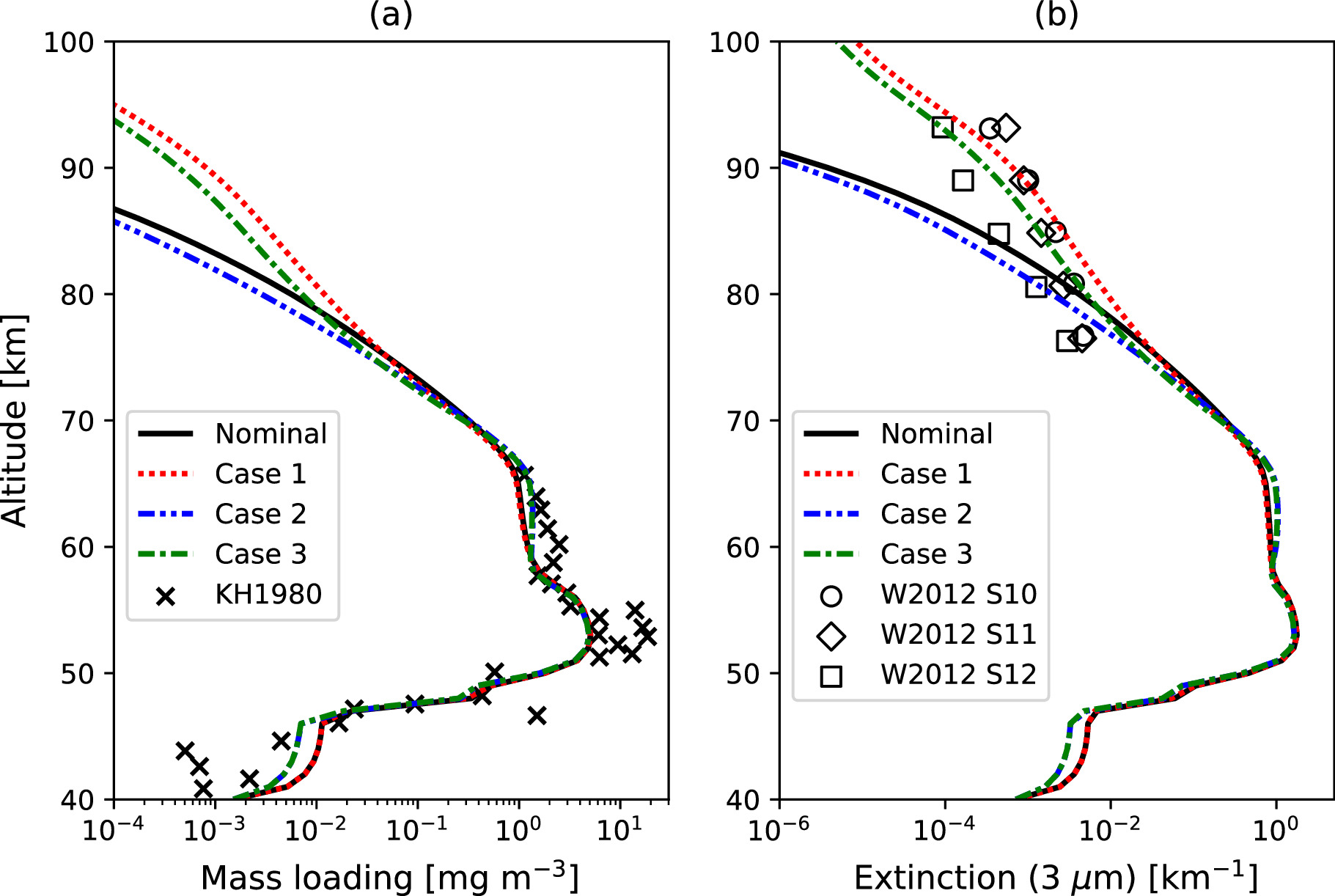
Figure 6. (a) Vertical profiles of the simulated mass loading (mg m−3) in the Nominal Case, Case 1 (red dotted line), Case 2 (blue double-dotted–dashed line), and Case 3 (green dashed–dotted line). The mass loading obtained by the LCPS (Knollenberg & Hunten 1980) is plotted for comparison as KH1980. (b) Vertical profiles of the simulated extinction coefficient (km−1) at 3 μm wavelength in the Nominal Case (black solid line), Case 1 (red dotted line), Case 2 (blue double-dotted–dashed line), and Case 3 (green dashed–dotted line) in comparison with the extinction coefficient at 3 μm wavelength measured by the VEx/SOIR (Wilquet et al. 2012) labeled as W2012 (season 10: S10; season 11: S11; season 12: S12).
Download figure:
Standard image High-resolution imageOn the other hand, the Nominal Case fails to replicate the observed extinction coefficient profile (Figure 6(b)). In the upper haze layer, the extinction coefficient decreases exponentially with altitude, but the simulated gradient is steeper than observed, resulting in values about two orders of magnitude smaller. The use of increased eddy diffusion coefficient in Cases 1 and 3 reduces the discrepancy with SOIR observations and results in a more extended upper haze layer. It is clearly shown that the cases with efficient eddy diffusion are in good agreement with the observed vertical profiles by Wilquet et al. (2012). This suggests that the recently estimated eddy diffusion coefficient (Mahieux et al. 2021) is suitable for the reproduction of the observed upper haze optical properties.
Figures 7 and 8 show the vertical profiles of condensational gas species. The H2SO4 VMR is fixed at 4 ppm at the bottom of the model and takes the maximum value of ∼6 ppm around the cloud bottom at 47 km for all cases (Figure 7(a)). This peak arises from droplet sedimentation in the lower cloud and subsequent evaporation. Between the cloud bottom and 60 km, the H2SO4 VMR aligns with the saturation vapor profile. This pattern agrees with observations from the Magellan mission (Kolodner & Steffes 1998) and recent VEx data (Oschlisniok et al. 2021), suggesting H2SO4 VMR levels of 5–7 ppm in the subcloud region at midlatitudes.
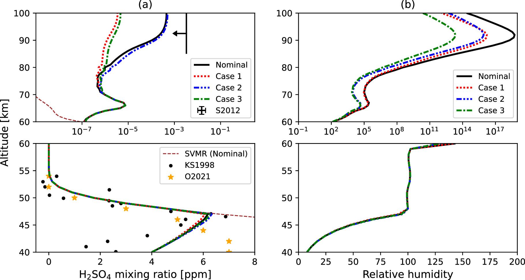
Figure 7. (a) Vertical profiles of the simulated H2SO4 VMR in the Nominal Case and Cases 1, 2, and 3 compared with the observations by Magellan radio occultation measurements (Kolodner & Steffes 1998; labeled as KS1998), VEx/VeRa measurements (Oschlisniok et al. 2021; labeled as O2021), and the upper limit suggested by Sandor et al. (2012; labeled as S2012). The saturation level of H2SO4 VMR (SVMR) is also indicated by a brown dashed line for the Nominal Case. (b) Vertical profiles of the simulated H2SO4 relative humidity in the Nominal Case and Cases 1, 2, and 3.
Download figure:
Standard image High-resolution image
Figure 8. Vertical profiles of the simulated H2O VMR in the Nominal Case and Cases 1, 2, and 3 compared with observations by SPICAV/SOIR (Fedorova et al. 2008), VIRTIS-H (Cottini et al. 2012), NASA Infrared Telescope Facility (Krasnopolsky et al. 2013), SPICAV/IR (Fedorova et al. 2016), and SPICAV/SOIR (Chamberlain et al. 2020), labeled as F2008, C2012, K2013, F2016, and C2020, respectively.
Download figure:
Standard image High-resolution imageAbove 75 km, the simulated H2SO4 VMR presents two distinct profiles. The first includes the Nominal Case and Case 2 scenarios with a maximum VMR of ∼5 × 10⁻⁴ ppm; the second includes Cases 1 and 3 with a maximum VMR of ∼5 × 10⁻⁶ ppm in the upper haze layer. The latter cases feature a higher eddy diffusion coefficient above 75 km, leading to a more abundant upper haze particle population. This facilitates condensation onto these particles, as the H2SO4 vapor is supersaturated. The peak values for both profile types are lower than the upper limit reported by Sandor et al. (2012), indicating that H2SO4 vapor is not a dominant source of sulfur species in the upper haze layer.
The H2SO4 VMR is supersaturated above 60 km and reaches its second-highest value at 67 km, due to the photochemical production of H2SO4 vapor across all cases. This finding is consistent with Dai et al. (2022), who used a cloud condensation model without detailed microphysics but assumed the same H2SO4 production profile as ours. These results indicate that the supersaturation above 60 km is a robust feature across different models when using the photochemical production of H2SO4 vapor from the 1D photochemical model of Krasnopolsky (2012). They further showed that if a Gaussian distribution is assumed for H2SO4 production, the H2SO4 VMR closely follows the saturation VMR in the upper haze layer. This is because the Gaussian distribution exhibits an extremely low value outside the half-width of the peak production altitude, and loss by H2SO4 condensation dominates over the photochemical production. The earlier work by Imamura & Hashimoto (2001), which also assumed a Gaussian profile, did not find supersaturation except near the peak production altitude. This sensitivity of the H2SO4 VMR profile to the assumed photochemical production profile suggests that it is a critical factor in modeling.
The H2O vapor VMR in the Nominal Case monotonically decreases from 40 to 67 km and stabilizes at ∼9 ppm above 67 km (Figure 8). This trend aligns qualitatively with VEx observations (Fedorova et al. 2008; Cottini et al. 2012; Fedorova et al. 2016), although the simulated values are slightly higher. The VMR gradient below the cloud base is steeper than in earlier work by Imamura & Hashimoto (2001) and recent microphysics model results reported by McGouldrick (2017) and McGouldrick & Barth (2023). The reason is that we use a lower eddy diffusion coefficient for those altitudes, based on the previous study by Woo et al. (1982). This steeper H2O VMR gradient helps balance the H2O vapor supply by upward eddy diffusion flux against loss from chemical reactions. In the lower and middle cloud layers, the gradient is less steep owing to stronger eddy diffusion, which acts to flatten the H2O vapor VMR profile. The mass fraction of liquid H2O in the droplets increases (corresponding to a decrease in liquid H2SO4 mass fraction, as shown in Figure 9(a)), indicating that the uptake of H2O vapor by the droplets also contributes to the decreasing H2O VMR from lower to upper cloud layers. Around 67 km, the H2O VMR experiences a sharp drop due to efficient chemical loss by H2SO4 formation (Equation (3) and Figure 1).
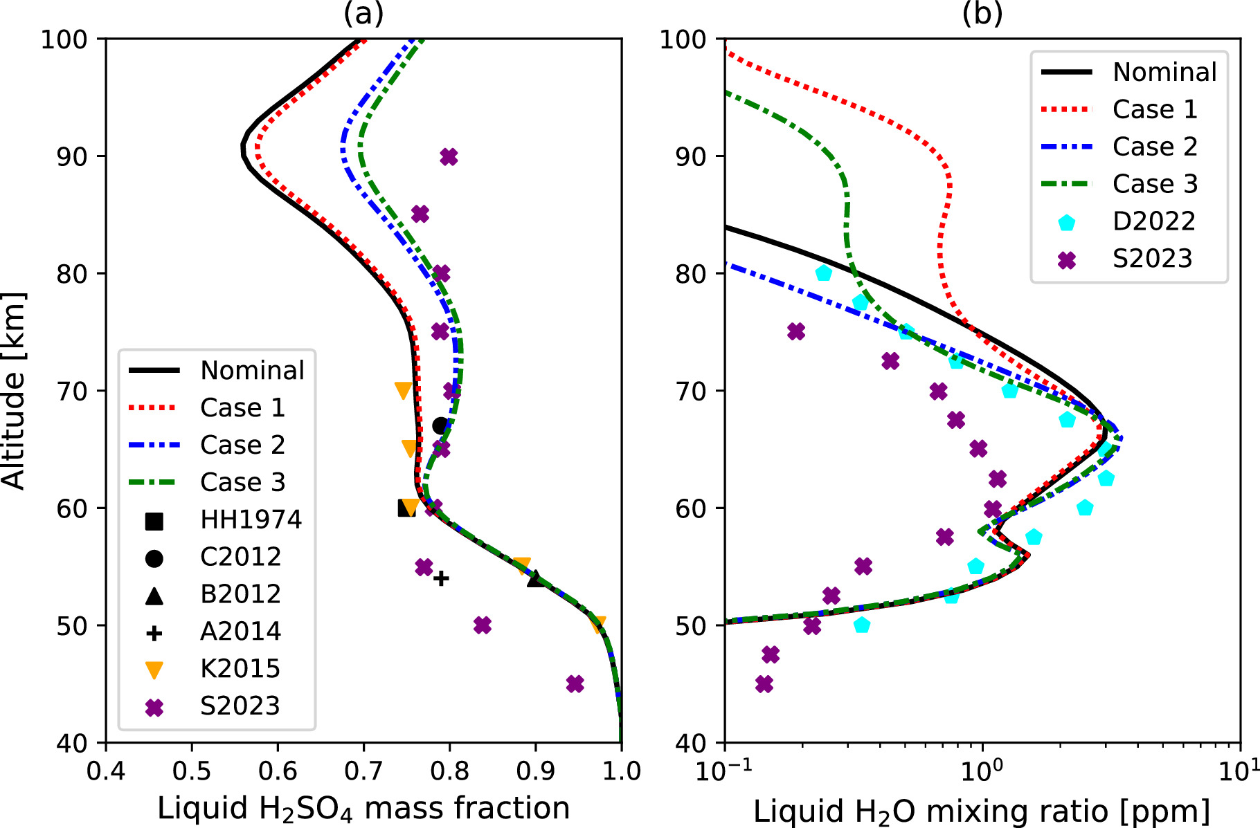
Figure 9. (a) Vertical profiles of the simulated liquid H2SO4 mass fraction in the Nominal Case and Cases 1, 2, and 3 in comparison with the modeling studies by Krasnopolsky (2015) and Stolzenbach et al. (2023), labeled as K2015 and S2023, respectively. The observations by Hansen & Hovenier (1974), Barstow et al. (2012), Cottini et al. (2012), and Arney et al. (2014) are labeled as HH1974, C2012, B2012, and A2014, respectively. (b) Vertical profiles of the simulated liquid-phase H2O VMR in the Nominal Case and Cases 1, 2, and 3 in comparison with the modeling studies by Dai et al. (2022) and Stolzenbach et al. (2023), labeled as D2022 and S2023, respectively.
Download figure:
Standard image High-resolution imageThe H2O VMR is highly sensitive to the assumed eddy diffusion profile used in the model (Figure 8). In Cases 2 and 3, the H2O VMR gradient is steeper between 60 and 70 km than in the Nominal Case and Case 1. Consequently, the H2O VMR decreases sharply in the upper cloud layer, aligning well with VEx observations (Fedorova et al. 2008; Cottini et al. 2012; Fedorova et al. 2016; Chamberlain et al. 2020) in these two cases. The defining feature of Cases 2 and 3 is the lower eddy diffusion coefficient between 60 and 70 km, suggesting that the mesospheric H2O vapor levels are influenced by the efficiency of eddy transport at these altitudes, as expected since the chemical loss of H2O is fixed.
Figure 9(a) shows liquid H2SO4 mass fraction in the cloud particles as a function of altitude. Below 50 km, the H2SO4 mass fraction exceeds 0.95 and decreases up to 60 km. It then stabilizes at ∼0.75 from 60 to 75 km in the Nominal Case and Case 1 scenarios, while increasing to ∼0.8 in Cases 2 and 3. The simulated values in the cloud layer are consistent with previous observations (Hansen & Hovenier 1974; Barstow et al. 2012; Cottini et al. 2012) in all cases. In particular, Cases 2 and 3 better match the data from Cottini et al. (2012). This vertical profile is also consistent with reported modeling studies (e.g., Krasnopolsky 2015; Stolzenbach et al. 2023), although our results are overestimated compared to Stolzenbach et al. (2023) below 60 km. Stolzenbach et al. (2023) argued that such a difference could be caused by the lower temperature bias of their model. Above 75 km, the H2SO4 mass fraction decreases again, reaching a minimum around 90 km before rising again up to the model top altitude for all cases. The decrease of the H2SO4 mass fraction between 75 and 90 km is attributed to a sharp temperature decrease, as temperature is the key factor determining thermal equilibrium.
The equilibrium condition is also influenced by the background H2O VMR, as the H2SO4 mass fraction adjusts to equilibrium through the uptake or release of H2O molecules at the particle surface. Therefore, a lower ambient concentration of H2O molecules results in reduced uptake by the droplets. As shown in Figure 8, the H2O VMR above 60 km is about an order of magnitude lower in Cases 2 and 3 compared to the Nominal Case and Case 1. This leads to less H2O being absorbed into the droplets and, conversely, a higher H2SO4 mass fraction within them.
Figure 9(b) shows the H2O VMR condensed in droplets as a function of altitude. Upon careful examination, the influence of eddy diffusion on the condensed H2O VMR is noticeable between 60 and 70 km. Specifically, the condensed H2O VMR is more concentrated at the cloud formation altitude around 66 km in Cases 2 and 3, due to the reduced eddy diffusion coefficient (see Figure 2). Above 70 km, Cases 1 and 3 exhibit higher levels of liquid H2O compared to the Nominal Case and Case 2. This is attributable to the extended aerosol layer in these two cases facilitated by the efficient eddy transport, leading to the upward transport of liquid H2O in its liquid phase. The condensed H2O VMR aligns well with the condensation model of Dai et al. (2022) in Cases 2 and 3. In their study, the liquid H2O VMR was ∼2 ppm in the upper cloud layer, ∼0.1 ppm at 50 km, and ∼0.2 ppm at 80 km. Note that the eddy diffusion profile they assumed was ∼0.3 m2 s−1 at 40 km, ∼1 m2 s−1 at 40–50 km, and 1–6 m2 s−1 at 60–70 km (see Table 4), resulting in a similar eddy transport timescale to our model.
Table 4. Comparison of Eddy Diffusion in This Study and Dai et al. (2022)
| Altitude (km) | Eddy Diffusion in Cases 2 and 3 (m2 s−1) | Eddy Diffusion in Dai et al. (2022) (m2 s−1) |
|---|---|---|
| 40 | 0.1 | ∼0.3 |
| 50 | 5 | ∼0.7 |
| 60 | 2 | 1 |
| 70 | 2 | ∼6 |
Download table as: ASCIITypeset image
A twofold difference in the eddy diffusion coefficient in the upper cloud layer leads to an order-of-magnitude difference in H2O VMR in the mesosphere, as shown in Figure 8. To investigate the sensitivity of H2O vertical profile with eddy diffusion, we compared the H2O flux profiles for the Nominal Case and Case 2 in Figure 10; positive fluxes indicate upward transport, and negative fluxes indicate downward transport. Below 60 km altitude, both profiles are identical since the eddy diffusion coefficient is nearly the same at these altitudes. It is noteworthy that the flux balances for the two cases are also similar between 60 and 70 km, even though the eddy diffusion coefficient for Case 2 is twice as large as that of the Nominal Case. Indeed, in a steady-state condition, the upward H2O vapor flux essentially balances with the sum of the liquid diffusion flux, liquid sedimentation flux, and cumulative chemical loss. However, as demonstrated in Figure 10(c), the difference in liquid flux between the two cases is relatively small, accounting for less than 20% difference in the total sum of the liquid flux and chemical loss. Given that the cumulative chemical loss is a constant parameter in all cases, the sums of the liquid flux and the cumulative chemical loss end up being similar. Consequently, the upward vapor fluxes are also similar, as they are balanced with the downward fluxes.
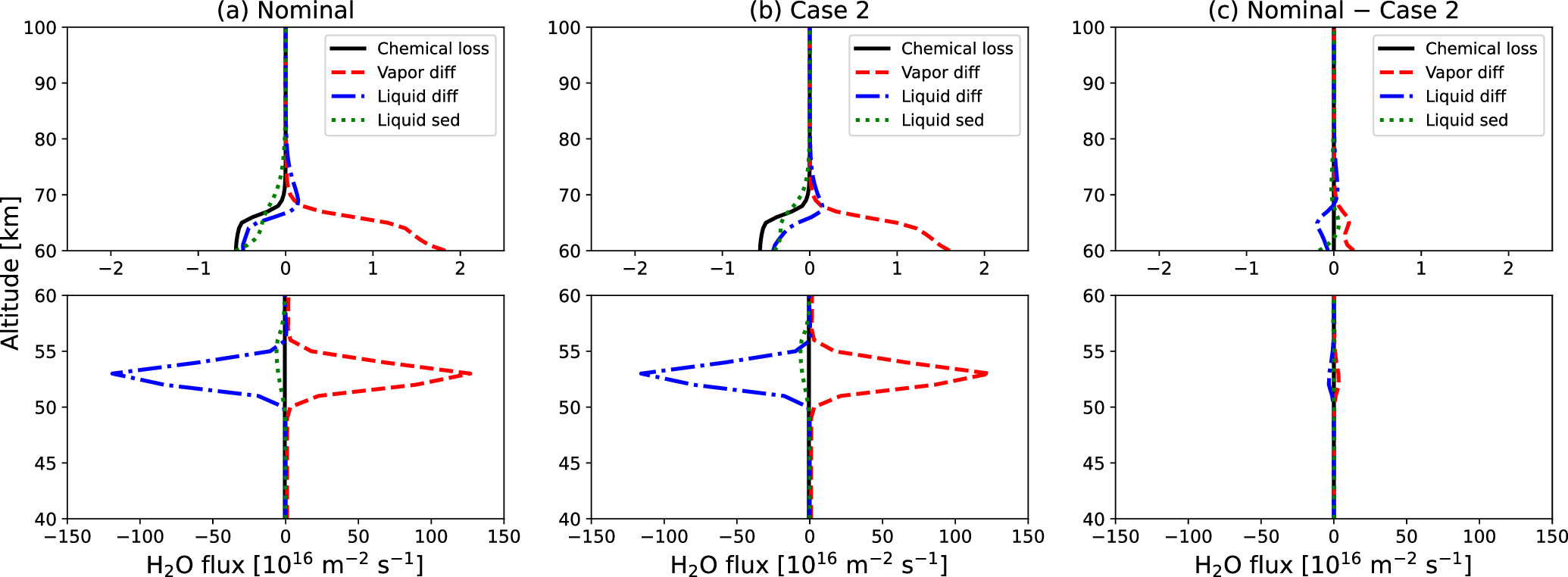
Figure 10. Vertical profiles of the simulated cumulative chemical loss of the H2O vapor (black solid line), H2O vapor diffusion flux (red dashed line), H2O liquid diffusion flux (blue dashed–dotted line), and H2O liquid sedimentation flux (green dotted line) in (a) the Nominal Case and (b) Case 2. (c) Difference of each flux between the Nominal Case and Case 2 (Nominal Case minus Case 2 values).
Download figure:
Standard image High-resolution imageThe two different H2O VMR trends shown in Figure 8 result from the fact that all cases exhibit similar upward H2O vapor fluxes between 60 and 70 km. In the present study, the species in the gas phase are transported only by eddy diffusion. The H2O vapor flux due to eddy diffusion  is expressed as
  , where Kzz
is the eddy diffusion coefficient, na
is the number density of air, and
, where Kzz
is the eddy diffusion coefficient, na
is the number density of air, and  is the H2O VMR. As shown in Figure 10,
  does not differ significantly in each case and can be regarded as a constant for simplicity. If Kzz
is increased by a factor of 2, the H2O VMR gradient
does not differ significantly in each case and can be regarded as a constant for simplicity. If Kzz
is increased by a factor of 2, the H2O VMR gradient  must be divided by 2 to yield the same vapor flux
  . This is why a twofold difference in the eddy diffusion coefficient leads to a significant change in the extent of H2O vapor depletion in the mesosphere. Consequently, the steep gradient reduces the H2O VMR in the upper cloud layer, leading to a H2O VMR that is about an order of magnitude smaller above 70 km in Cases 2 and 3.
In the present study, the chemical production/loss rate of condensational gas species is fixed. However, as shown in Figure 10, the cumulative H2O chemical loss also plays a significant role in determining the compensating upward H2O vapor flux. Namely, if the chemical loss rate is increased and Kzz
is fixed,  should increase to balance with the chemical loss. Given the amplitude of the cumulative chemical loss compared to the liquid flux components, it is expected that a factor of variation of the loss rate may lead to considerable change in
  .
.
The recent cloud condensation model from Dai et al. (2022) showed a similar relationship between eddy diffusion and the H2O gradient in the upper cloud layer. With the same H2O chemical loss profile as in our study, the Nominal Case from Dai et al. (2022) used an eddy diffusion coefficient of 1 m2 s−1 at 60 km and ∼3 m2 s−1 at 65 km. This suggests that the efficiency of eddy transport in their study aligns closely with ours. Their resulting H2O VMR gradient between 60 and 70 km was steep enough to reduce the H2O VMR to a few parts per million at 70 km. In contrast, when they used the eddy diffusion profile from Bierson & Zhang (2020), which had a value of ∼4 m2 s−1 between 60 and 70 km, they observed a less steep H2O gradient. The resulting H2O VMR exceeded 10 ppm at 70 km. Our results also overestimated the H2O VMR at 70 km when the eddy diffusion is set to 4 m2 s−1 between 60 and 70 km. The similarities between our findings and those from Dai et al. (2022) highlight the critical role of the eddy diffusion coefficient in the upper cloud layer. Furthermore, both studies concur that an eddy diffusion of ∼2 m2 s−1 serves as a threshold beyond which hygroscopic effects become significant.
The influence of eddy diffusion on the chemical production/loss rates should also be explored. It has been established that the vertical profiles of sulfur species are significantly influenced by eddy diffusion. Krasnopolsky (2012) demonstrated that variations in eddy diffusion coefficients above 55 km can lead to a significant difference in SO2 concentrations in the upper cloud region. Additionally, Bierson & Zhang (2020) found that the altitude and rate of H2SO4 production vary considerably with the eddy diffusion coefficient in the cloud layers. Given the vital role of the chemical production profile in the formation of the upper cloud and the depletion of H2O, the H2SO4 and H2O fluxes could be altered by the response of sulfur chemistry to eddy diffusion. However, here we focus on the impact of changing eddy diffusion on cloud microphysics and its effect on the H2SO4 and H2O fluxes, and the coupling between photochemistry and cloud microphysics will be addressed in future research.
3.2. Sensitivity to Upper Temperature Profiles
We examined the sensitivity of aerosol and gas species distributions to variations in the upper temperature profile by comparing the VIRA temperature cases (Nominal Case and Case 3) and the SOIR temperature cases (Cases 4 and 5). The mass loading and extinction coefficient in both scenarios are very similar up to 80 km and in good agreement with the LCPS observations, as shown in Figure 11. Above 80 km, the upper haze is more extended in Cases 3 and 5 because both cases use the updated eddy diffusion by Mahieux et al. (2021), which is consistent with the results shown in Section 3.1. However, we observed that the population of the upper haze particles is slightly reduced when using the temperature profile from SOIR. As will be discussed later, this reduction is due to the aerosol evaporation, which is triggered by the warm layer evident in the SOIR temperature profile.
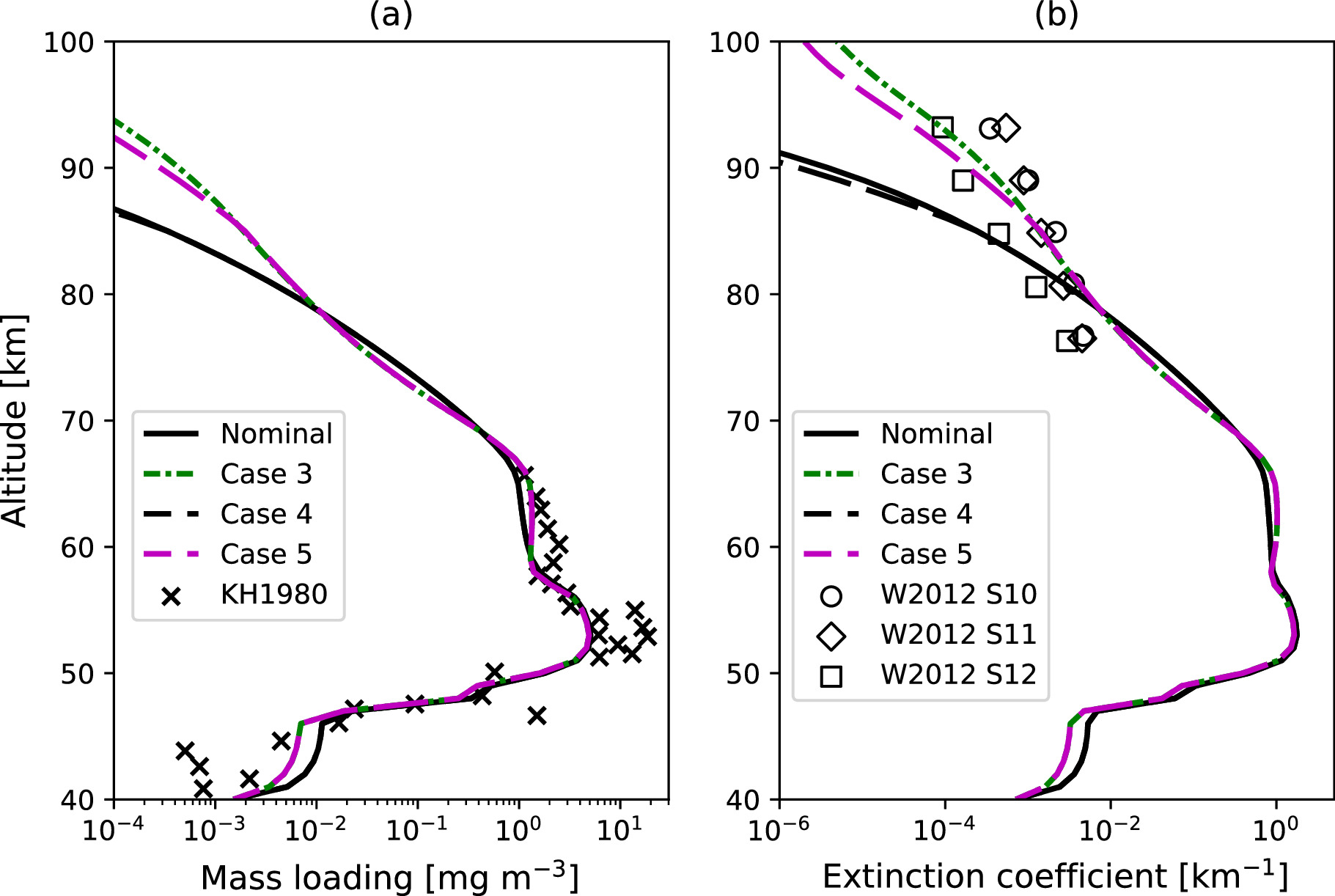
Figure 11. Same as Figure 6, but the simulated results for Cases 4 and 5 are added with black and magenta dashed lines, respectively, and the Case 1 and 2 results are removed for visibility.
Download figure:
Standard image High-resolution imageThe H2SO4 VMR in Case 5, which uses the SOIR temperature profile, closely resembles that of Case 3 up to ∼85 km altitude but diverges significantly from Case 3 above 85 km (see Figure 12(a)). On the other hand, the H2SO4 VMR in Case 4 is larger than the Nominal Case, but the amplitude is much less pronounced. The saturation H2SO4 VMR calculated using the SOIR profile (Case 5) is orders of magnitude higher than the one calculated using the VIRA profile, as the maximum temperature of the SOIR profile is up to ∼50 K higher than that in the VIRA profile. Due to this elevated saturation VMR, the H2SO4 vapor is undersaturated in the upper haze layer above ∼90 km in Cases 4 and 5 (Figure 12(b)). This undersaturation leads to the evaporation of the upper haze particles, in turn increasing the H2SO4 VMR in the SOIR temperature cases. However, the deviation from VIRA temperature case is more evident in Case 5 than in Case 4 because the extended upper haze layer supplies H2SO4. As a result of the combined effect of enhanced eddy diffusion and higher temperature, the H2SO4 VMR aligns with the upper limit suggested by Sandor et al. (2012) in Case 5, suggesting that the mesospheric H2SO4 vapor could be detectable under high-temperature conditions.

Figure 12. Same as Figure 7, but the simulated results for Cases 4 and 5 are added with black and magenta dashed lines, respectively, and the Case 1 and 2 results are removed for visibility. The saturation level of H2SO4 VMR (SVMR) is also indicated by a cyan dashed line for Case 4 in panel (a).
Download figure:
Standard image High-resolution imagePrevious photochemical studies suggested that ∼1 ppm of H2SO4 vapor is required to act as a precursor for SO2 and SO in the upper haze layer (Zhang et al. 2010, 2012). However, the simulated values are orders of magnitude lower than this suggested value, even when using the SOIR temperature (see Figure 12(a)). This discrepancy raises the possibility that sources other than H2SO4 aerosol may be needed to provide sufficient sulfur, such as elemental sulfur suggested by Zhang et al. (2012).
The H2O VMR in Case 4 does not deviate from that obtained in the Nominal Case, as also seen in H2SO4 VMR. This is due to the lack of aerosols in the upper haze layer in both cases. However, when Cases 3 and 5 are compared, the H2O VMR simulated with the SOIR temperature profile diverges notably from that simulated using the VIRA profile, especially above ∼85 km (Figure 13). In Case 5, the H2O VMR reaches a minimum value at ∼85 km and then increases with altitude. This pattern aligns with the H2O VMR profile observed by Fedorova et al. (2008) and Chamberlain et al. (2020). The increase in H2O VMR above 85 km can be attributed to the strong dependence of equilibrium conditions on the background temperature. It is important to note that the diverging altitude can vary depending on how the temperature profile is constructed in the model and may also change when taking into account the interprofile variability discussed in Section 2.3.

Figure 13. Same as Figure 8, but the simulated results for Cases 4 and 5 are added with black and magenta dashed lines, respectively, and the Case 1 and 2 results are removed for visibility.
Download figure:
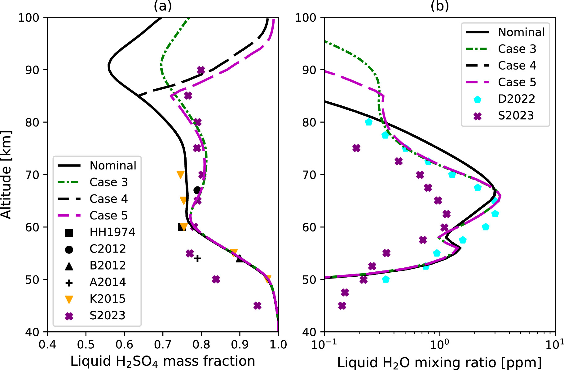
Standard image High-resolution imageThe equilibrium condition manifests in the liquid H2SO4 mass fraction within the droplets. In Cases 4 and 5, there is a significant increase in the H2SO4 mass fraction above 85 km, corresponding to the sharp temperature increase in the SOIR profile (Figure 14(a)). This suggests that the droplets cannot maintain a high H2O content above this altitude. The reduced liquid H2O VMR in the droplets is corroborated in Case 5 (Figure 14(b)). Specifically, the liquid H2O VMR experiences a sharp decline above 85 km. This implies that there are more H2O molecules in gas phase in the SOIR temperature scenario compared to the VIRA temperature case because of the warm layer that leads to H2O evaporation. Thus, the increasing H2O VMR in Figure 13 can be attributed to the release of the H2O molecules from the upper haze particles that have been transported upward from below 85 km.
Figure 14. Same as Figure 9, but the simulated results for Cases 4 and 5 are added as the black and magenta dashed lines, respectively, while Cases 1 and 2 are removed for visibility.
Download figure:
Standard image High-resolution image
4. Discussion
4.1. Best-fit Atmospheric Parameters
In Section 3.1, we identified a strong dependence of both aerosol and gas species distributions on the eddy diffusion profiles. The aerosol distribution is highly sensitive to the eddy diffusion coefficient above 85 km (Figure 6). Results for Cases 1 and 3, using the eddy diffusion recently estimated by Mahieux et al. (2021), closely match the upper haze distribution observed by SOIR (Wilquet et al. 2012). Furthermore, Cases 2 and 3 using lower eddy diffusion coefficients between 60 and 70 km are consistent with the observed H2O VMR distribution reported by VEx observations (Fedorova et al. 2008; Cottini et al. 2015; Fedorova et al. 2016; Chamberlain et al. 2020). Given that Case 3 successfully reproduces both the observed gas species and aerosol distributions, the present study suggests that the eddy diffusion should be ∼360 m2 s−1 in the upper haze layer and ∼2 m2 s−1 in the upper cloud layer, when the chemical production/loss rates of condensational species are fixed.
In our study, as mentioned earlier, the eddy diffusion includes global transport processes such as Hadley-type circulation since our model represents the whole atmosphere with a 1D column. To compare the eddy diffusion coefficient obtained in the present study with those derived from the general circulation model (GCM), we employ timescale estimations. The eddy transport timescale is given by τ = H2/Kzz , where H is the scale height of the atmosphere. On the other hand, the timescale of the global-scale circulation can be estimated by τ = H/w, where w is the typical vertical wind speed. Assuming that eddy transport is mainly driven by the global-scale circulation, the relationship Kzz = H w can be derived. Takagi et al. (2018) obtained a zonally and temporally averaged vertical wind speed magnitude on the order of ∼0.001 m s−1 at 70 km using Atmospheric GCM for the Earth Simulator for Venus (AFES-Venus). With a corresponding scale height of 5 km, these values yield Kzz = 5 m2 s−1, which is within the same order of magnitude as the eddy diffusion coefficient assumed between 60 and 70 km in the present study. Navarro et al. (2021) found a zonally and temporally averaged vertical wind speed magnitude on the order of ∼0.1 m s−1 at 90 km using the Institut Pierre-Simon Laplace (IPSL) GCM, and the scale height at the corresponding altitude is ∼3.7 km. These two values give Kzz = 370 m s−1, which is equivalent to the eddy diffusion coefficient assumed above 85 km in our study. A GCM study by Sugimoto et al. (2019) showed that vertical eddy diffusion coefficients due to small-scale turbulences should be less than 0.02 m2 s−1 to reproduce realistic super-rotation. This value is significantly smaller than the eddy diffusion derived using the above formulation. This could suggest that global-scale circulation effectively represents the eddy diffusion transport in a 1D column. Specifically, the dynamical timescales obtained in the GCMs are consistent with the timescale required to reproduce observed cloud structure and condensational gas species. Above 85 km, the existence of subsolar-to-antisolar (SSAS) circulation is supported by observations of O2 nightglow at the antisolar point (Soret et al. 2012) and the Venus Thermospheric GCM (e.g., Brecht et al. 2012; Hoshino et al. 2013; Navarro et al. 2021). Thus, the large eddy diffusion above 85 km may be attributed not only to Hadley-type circulation but also to the influence of the SSAS circulation.
The case studies showed that the H2O VMR profile is highly sensitive to the eddy diffusion coefficient between 60 and 70 km. The eddy diffusion coefficient used in this study is broadly consistent with previous observations and numerical models. Therefore, a thorough examination of the eddy diffusion coefficient in this altitude range is crucial for understanding H2O transport through the cloud layer. Numerical investigations of the eddy diffusion coefficient can be performed using a GCM, as shown by Zhang & Showman (2018). Recently, Fujisawa et al. (2022) achieved a realistic representation of wind and thermal structures using a data assimilation technique that combines AFES-Venus and AKATSUKI observations. Such data assimilation products could serve as valuable resources for deriving an eddy diffusion coefficient that accounts for both global and local transport processes.
In terms of the mesospheric temperature, the SOIR profile is more suitable to reproduce the observed H2O VMR increase above 85 km (see Figure 13). Therefore, the present study suggests that Case 5 provides the best match with observed atmospheric parameters. However, observed temperature profiles appear to differ depending on the instrument used for observation. In general, radio occultation measurements yield lower temperature profiles compared to those obtained through infrared observations (Limaye et al. 2018), as depicted in Figure 3(a). In addition, Krasnopolsky (2011) argued that high temperatures between 95 and 100 km disagree with the rotational temperature of the O2 nightglow at 1.27 μm.
This discrepancy could potentially be resolved by measuring the liquid H2SO4 mass fraction in upper haze particles. As shown in Figure 9(a), the liquid H2SO4 mass fraction varies significantly depending on the temperature—a variation that should be detectable. Consequently, we can use the H2SO4 mass fraction as a proxy to better understand the upper-mesospheric temperature profiles and the resulting equilibrium conditions. However, as Mahieux et al. (2023b) pointed out, the temperature difference could be caused by the local time dependence. In that case, the temperature observations can be used as a proxy for the H2SO4 mass fraction of aerosols. Regardless of the scenario, acquiring more detailed observations that focus on the local time dependence of mesospheric temperatures is crucial for enhancing our understanding of the microphysical properties of aerosols.
4.2. Implication for Atmospheric Evolution
The H2O abundance at the homopause regulates the hydrogen (H) escape rate through diffusion-limited flux. Assuming a H2O vapor abundance of ∼1 ppm and HCl of ∼0.5 ppm at the homopause, the diffusion-limited flux is calculated to be ∼3 × 10¹¹ m−2 s−1 (Catling & Kasting 2017). This value is consistent with an estimate of the nonthermal escape flux of ∼3 × 10¹¹ m−2 s−1 (Lammer et al. 2006), indicating that the diffusion-limited flux serves as a good approximation for estimating the present-day H escape flux. Therefore, the H2O vapor abundance at the homopause is crucial for understanding the current atmospheric evolution of Venus.
The long-term stability of the Venusian clouds is still controversial. Bullock & Grinspoon (2001) showed that the clouds would not be stable if the atmospheric SO2 amount is buffered by carbonate. Conversely, Hashimoto & Abe (2005) argued that the clouds would be stable if the atmospheric SO2 amount is buffered by pyrite. These contrasting scenarios could lead to significant differences in H2O loss rates, given that the cloud layer affects the diffusion-limited escape rate. Therefore, the presence of clouds and their impact on mesospheric H2O abundance should be carefully considered in models of Venusian atmospheric evolution. The present study shows that cloud processes are essential to evaluate the H2O VMR vertical profile, which is deeply connected to H2O vapor abundance at the homopause. Consequently, cloud processes cannot be disregarded when studying the mesospheric H2O abundance and the diffusion-limited escape rate. These cloud effects should be considered not only for the present-day atmosphere but also for the past atmospheric conditions. Furthermore, observations of trace gas species and clouds, possible with the future EnVision mission, will further elucidate the effects of clouds on atmospheric evolution (e.g., Widemann et al. 2023). The VenSpec-H instrument on board the Envision spacecraft will observe H2O abundance below and above the cloud layer with high accuracy, and the Radio Science experiment will obtain liquid H2SO4 abundance in the cloud layer (Akins et al. 2023). This information will allow the community to investigate the role of clouds in regulating the mesospheric H2O abundance and its impact on the hydrogen escape.
4.3. Bimodal Distribution in the Upper Haze Layer
The simulated size distribution in the upper haze layer is unimodal, diverging from the bimodal distribution suggested by VEx observations (Wilquet et al. 2009). Previous microphysics studies (Gao et al. 2014; Parkinson et al. 2015) have also reported unimodal distributions in the upper haze layer at steady state. However, Gao et al. (2014) argued that transient vertical winds could give rise to the observed bimodal distribution. The inclusion of dynamical effects, which is not considered in the present study, may be necessary to accurately reproduce the observed particle size distribution and should be explored in future research.
Homogeneous nucleation processes could play a significant role in the generation of the Mode 1 particles. Dai et al. (2022) obtained a supersaturated H2SO4 VMR profile in the upper cloud and haze layer, which aligns with the findings of our study; their results were obtained using a cloud condensation model. They argued that under such a supersaturated condition homogeneous nucleation is likely to occur. The enhanced CN population could correspond to Mode 1 particles, as observed in the lower and middle cloud layers of the recent microphysical model (McGouldrick & Barth 2023). This idea is supported by the VIRA temperature cases (Nominal Case and Cases 1–3), where the H2SO4 vapor is highly supersaturated in the upper haze layer, as shown in Figure 7(a). The potential for homogeneous nucleation should be further explored using a cloud microphysics model that includes CN size distributions in future studies.
5. Summary and Conclusions
We developed a 1D cloud microphysics model based on the work of Imamura & Hashimoto (2001) and extended the model top altitude from 70 to 100 km. The temperature and pressure profiles are adapted from the midlatitude profiles from VIRA (Seiff et al. 1985) to represent the global average atmosphere. We updated the production rate of H2SO4 vapor using recent photochemical model results (Krasnopolsky 2012). The simulated size distribution and mass loading are in good agreement with in situ observations (Knollenberg & Hunten 1980) and successfully replicate the earlier work by Imamura & Hashimoto (2001). A sharp peak of the H2SO4 VMR forms below the clouds, reaching a value of ∼6 ppm, which is quantitatively consistent with previous observations (Kolodner & Steffes 1998; Oschlisniok et al. 2021).
To investigate the transport processes of gas species and aerosols, we conducted case studies consisting of four distinct eddy diffusion patterns. These patterns were created using a pair of small and large eddy diffusion coefficients between 60–70 km and 85–100 km. When using the recently updated eddy diffusion coefficient from Mahieux et al. (2021) in the upper haze layer (85–100 km), the aerosol extinction coefficient is in good agreement with VEx/SOIR observations (Wilquet et al. 2012), indicating that efficient dynamical transport is essential for maintaining this layer. The H2O vapor profile is consistent with VEx/SOIR observations (Fedorova et al. 2008) when the eddy diffusion coefficient in the upper cloud layer is halved relative to previous radio scintillation measurements (Woo & Ishimaru 1981). The H2O VMR is highly sensitive to changes in eddy diffusion at these altitudes, as the gradient of H2O VMR profile varies significantly depending on the eddy diffusion coefficient. The H2SO4 VMR in the upper haze layer is also highly sensitive to the eddy diffusion coefficient above 85 km, ranging from ∼5 × 10⁻⁶ (5 ppt) to ∼5 × 10⁻⁴ ppm (0.5 ppb). However, the simulated values are orders of magnitude lower than the observational upper limit suggested by Sandor et al. (2012) across cases using the VIRA temperature vertical profile.
To investigate the impact of temperature on gas species and aerosol distributions, we conducted an additional case study using a temperature profile obtained by VEx/SOIR (Mahieux et al. 2015, 2023b). Due to the presence of a warm layer in the SOIR temperature profile, the H2SO4 VMR increases to ∼3 ppb above 90 km, as the elevated temperature raises the H2SO4 saturation pressure. However, when compared to the photochemical modeling results of Zhang et al. (2010), the elevated H2SO4 VMR is still insufficient to account for the observed SO2 inversion layer. In the upper haze layer, the liquid H2SO4 mass fraction in the aerosols shows a notable increase compared to the VIRA-based case and H2SO4 vapor reaches the upper limit of 3 ppb measured by Sandor et al. (2012).
The present study identifies the best-fit eddy diffusion coefficients as ∼360 m2 s−1 above 85 km and ∼2 m2 s−1 between 60 and 70 km. Updating the eddy diffusion coefficient in the 60–70 km altitude range is essential for understanding the transport dynamics of H2O vapor through the cloud layers. In addition, it is also expected that the increase of H2SO4 production rate enhances H2O loss, which results in the depletion of H2O above the upper cloud layer. Such updates could be achieved through numerical investigations using data assimilation products or future missions. In addition, this study suggests that the H2O VMR profile is better replicated using the SOIR temperature profile. However, previous observations have shown variability in the temperature profiles in the upper haze layer depending on the instrument used for observation. Measuring the liquid H2SO4 mass fraction in droplets could serve as a discriminative factor for validating temperature profiles and establishing the equilibrium conditions in the upper haze layer.
This study shows that the mesospheric H2O abundance is affected by the transport in the upper cloud layer, which could potentially regulate the diffusion-limited escape rate. Therefore, we suggest that the effects of clouds should be included in models of Venus's atmospheric evolution. In addition, the formation of Mode 1 particles in the upper haze layer could be linked to homogeneous nucleation processes. These topics warrant further investigations through more sophisticated cloud microphysics models in future studies.
Acknowledgments
This study was supported by the Japan Society for the Promotion of Science (JSPS) (KAKENHI grant Nos. JP23KJ0201, JP23H01236, JP22H00164, JP20H01958, JP19H05605, and JP19K14789), the Fusion Oriented REsearch for disruptive Science and Technology (FOREST) Program of the Japan Science and Technology Agency (JST) (grant No. JPMJFR212U), the Astrobiology Center of National Institutes of Natural Sciences (NINS) (grant No. AB0509), and the International Joint Graduate Program in Earth and Environmental Sciences (GP-EES) of Tohoku University. Venus Express is a planetary mission from the European Space Agency (ESA). We thank all ESA members who participated in the mission, particularly H. Svedhem and D. Titov. We thank our collaborators at IASB-BIRA (Belgium), Latmos (France), and IKI (Russia). The research program was supported by the Belgian Federal Science Policy Office and the European Space Agency (ESA, PRODEX program, contracts C 90268, 90113, 17645, 90323, and 4000107727). A.M. was supported by the Marie Skłodowska-Curie Action from the European Commission under grant No. 838587. S.V. was supported by the Belgian Science Policy Office through the BrainBe MICROBE Project Project under grant No. B2/191/P1/MICROBE.