

Abstract
Agrivoltaic systems that locate crop production and photovoltaic energy generation on the same land have the potential to aid the transition to renewable energy by reducing the competition between food, habitat, and energy needs for land while reducing irrigation requirements. Experimental efforts to date have not adequately developed an understanding of the interaction among local climate, array design and crop selection sufficient to manage trade-offs in system design. This study simulates the energy production, crop productivity and water consumption impacts of agrivoltaic array design choices in arid and semi-arid environments in the Southwestern region of the United States. Using the Penman–Monteith evapotranspiration model, we predict agrivoltaics can reduce crop water consumption by 30%–40% of the array coverage level, depending on local climate. A crop model simulating productivity based on both light level and temperature identifies afternoon shading provided by agrivoltaic arrays as potentially beneficial for shade tolerant plants in hot, dry settings. At the locations considered, several designs and crop combinations exceed land equivalence ratio values of 2, indicating a doubling of the output per acre for the land resource. These results highlight key design axes for agrivoltaic systems and point to a decision support tool for their development.
Export citation and abstract BibTeX RIS

Original content from this work may be used under the terms of the Creative Commons Attribution 4.0 license. Any further distribution of this work must maintain attribution to the author(s) and the title of the work, journal citation and DOI.
1. Introduction
Agrivoltaics, the practice of co-locating photovoltaic arrays and agricultural production on the same land, is of growing interest as the world transitions to renewable energy (Macknick et al 2022). Historically, more than half of the land used for photovoltaic production is converted from crop production (Kruitwagen et al 2021), and photovoltaics could occupy 10% or more of the land currently used for crops in some regions by 2050 (OECD/IEA 2021, van de Ven et al 2021). Agrivoltaics presents the opportunity to reduce the competition between food and energy needs for scarce land resources (Dupraz et al 2011, Barron-Gafford et al 2019). Results from initial agrivoltaic pilot projects suggest system benefits from interactions between the crop and solar array can make agrivoltaics competitive relative to conventional solar arrays and, in some cases, conventional agriculture (Amaducci et al 2018, Barron-Gafford et al 2019, Agostini et al 2021)
The central challenge of agrivoltaics is apportioning sunlight among the crop and the photovoltaic panels to support adequate crop and electricity production. To date, the agrivoltaics field has not systematically evaluated design approaches—largely because the optimal partition of sunlight depends on geography and crop selection. Implementations range from low density, semi-transparent panels at high coverage levels to vertically oriented, widely spaced bifacial panels that provide negligible shading and obtain substantial illumination from reflected light (Elamri et al 2018, Othman et al 2020, Ott et al 2020, Riaz et al 2020, Abidin et al 2021, Agostini et al 2021, Trommsdorff et al 2021). The diversity of agrivoltaic pilot projects reflects agricultural diversity, but translating the knowledge between settings is challenging without understanding the interplay between system components and the effect of local climate conditions on those interactions. Current models neglect key drivers of plant function and thereby overlook critical features of agrivoltaic system interactions.
Agrivoltaic researchers have adopted the concept of the land equivalence ratio (LER) from intercropping systems (Mead and Willey 1980, Trommsdorff et al 2021). This nondimensional metric is equal to the amount of land required to replicate the agrivoltaic system's yield of electricity (in kW-hr yr−1) and crops (in the metric appropriate for the specific crop considered) using conventional solar array and agricultural practices on separate land plots (equation (1)),
While this metric is succinct, it reduces all performance comparison to land savings. Important for dryland regions, the LER approach neglects the impact on water consumption—the primary limiting factor in food production (Jaeger et al 2017). The addition of a photovoltaic array directly affects soil evaporation and crop transpiration, collectively known as evapotranspiration (ET), by altering the radiation environment. Because freshwater withdrawals already exceed 100% of renewable water resources in some regions, the impact of agrivoltaics on water consumption is a crucial metric.
The agrivoltaics field has begun building on existing modeling frameworks developed for photovoltaics (Usama Siddiqui et al 2012, Liu et al 2016, Jain et al 2017) and agronomy (Valiantzas 2013, Jones et al 2017) to predict crop and energy production for integrated systems. To date, these efforts have fallen into two categories. In one, modelers apply a light response curve combined with the reduction in photosynthetically active radiation (PAR) caused by shading (Campana et al 2021, Trommsdorff et al 2021, Riaz et al 2022), thereby neglecting vital plant physiology determinants of performance and simply predicting a decline in crop productivity with increasing array coverage. These simulations predict a direct tradeoff between food and energy production in the settings considered but have not explored climate contributions to agrivoltaic performance. The second modeling approach uses parameterized crop models (Amaducci et al 2018, Elamri et al 2018) tying these models to specific input and location cases. These more physiologically detailed efforts have considered a fixed array architecture and emphasized finding crop partners for agrivoltaics accompanied by experiment. These endpoints of model complexity leave a gap in ability to evaluate and predict whole system performance.
Here we evaluate the effects of array design and crop selection on agrivoltaic energy production, crop production, and water use in three case study locations in the southwestern United States. We present a new intermediate modeling approach that adds a temperature response to the light response component and estimates water use. The goals of the analysis are to identify array design characteristics that minimize impacts to crop productivity and maximize savings of irrigation water. We anticipate identifying some system configurations that increase crop productivity in tandem with significant water savings in arid environments. Finally, we combine the analysis of energy production from the arrays to determine a trade-off with electricity generation for array designs that maximize crop productivity or water savings.
2. Methods
2.1. Modeling approach
We approach the question of how an agrivoltaic array will affect water consumption and plant growth by determining how the array changes the illumination conditions in the field and then applying those illumination conditions to (1) a model of ET and (2) a plant productivity model (figure 1). The same calculation captures the illumination of the photovoltaic panels and hence the electricity production. The model is implemented in MATLAB (MathWorks). For simplicity, the model assumes conditions under the array are the same as the control setting in all aspects other than illumination. While multiple studies have reported differences in air temperature in the presence of photovoltaic arrays (Barron-Gafford et al 2019, Broadbent et al 2019, Jiang et al 2021), the effects are not consistent in magnitude or sign across or within studies. To examine the sensitivity of the results to this assumption, we also considered scenarios where the air temperature under the array differed from the ambient by up to ±5 °C (see supplemental).

Figure 1. Schematic representation of modeling scheme for this study. User-selected inputs of array geometry, time and location are used to calculate the shade pattern at six minute intervals. The agrivoltaic shading is in turn used to determine electricity and crop production and water consumption in combination with data on local solar and climate conditions. The model combines electricity and crop production to determine the land equivalence ratio (LER), which, along with the water consumption, is the model output.
Download figure:
Standard image High-resolution image2.2. Array geometry and shading
The first modeling step generates an array geometry based on the unit panel dimensions, the panel orientation (azimuth and tilt angle) and the panel height (figure 2(a)). The array unit cell includes the unit panel (2 m wide and 1.3 m in height, elevated 2.5 m) and variable space, tiled two directions (figure 2(b)). The analysis considered array rows of either North-South (NS) or East-West (EW) axes. We also examined three panel tilt angles, 0, 20 and 30 degrees to the South (for EW rows) or West (for NS rows). Together, these design permutations span the density and orientation of most fixed-panel solar installations and includes average tilt angles for latitudes up to approximately 45 degrees.
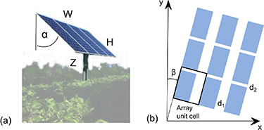
Figure 2. Schematic view of agrivoltaic array parameters that can be varied within the model. In panel (a), dimension of panel width, W and height (H); mounting height (Z); and mounting angle (α). As the image shows, the panel may be composed of multiple photovoltaic devices in one unit, depending on the design. In panel (b), the array parameters: angle of row (β) relative to ordinal directions, spacing between rows (d1) and spacing between panels within rows (d2). The array unit cell illustrates the element tiled in two directions to create the full array.
Download figure:
Standard image High-resolution imageArray coverage (projected area of the panels from nadir divided by the field area) ranges from 100% to 1% and is the primary basis of comparison between the designs in the subsequent analysis. To generate the shade pattern, we first calculated the solar angle at six-minute intervals for each day of the year at each location (Blanco-Muriel et al 2001). We determined the shade fraction by comparing the area of the panel shadow projected onto the ground plane to the area of the array unit cell. Any self-shading by adjacent panels was corrected in total shading and electricity production calculations.
2.3. Modeling of water consumption
We model the array impact on ET using the FAO formulation of the Penman–Monteith equation (equation (2)) (Allen et al 1998).
This model estimates the ET of a plant layer based on the energy balance between incoming solar radiation (G), outgoing thermal radiation (Rn ), and latent heat from ET, as governed by the local air conditions: vapor pressure deficit (es –ea ), the air density (ρa ), specific heat (cp ), psychrometric constant (γ) and slope of the vapor saturation pressure curve (Δ), and bulk and aerodynamic resistances (rs and ra ) that represent the restrictions to water transport through the soil, plant tissues and canopy.
For full sun ET estimates, G is the global horizontal irradiance, and for full shade conditions, G is the diffuse irradiance, both taken from the National Solar Radiation Database (Sengupta et al 2018). We assume that the leaf surface temperature is equal to the air temperature, the sky temperature is 273 K and the albedo is 0.7, which together determine the outgoing radiation (Rn ) (Evangelisti et al 2019). Temperature, ambient water vapor pressure and wind speed are hourly climate normals for the location, interpolated for model timesteps (Arguez et al 2012). The surface roughness/diffusivity parameters of the PM model, ra and rs , are the baseline values for grass (Allen et al 1998).
To analyze water savings for each array case, we weighted the baseline full sun and full shade ET rates at each timestep by the sun and shade fractions and calculated an average ET rate for the field as a whole. This instantaneous ET rate was then integrated over each day or the total year to quantify seasonal and cumulative trends.
2.4. Modeling of crop productivity
As in many current ecosystem modeling efforts, our model avoids distinguishing among plant species, but rather collapses plant differences into two broad types: shade-tolerant plants and sun-tolerant plants. Productivity in our model refers to photosynthetic activity, which we treat as a proxy for all crop products. We assume that the plants are managed to avoid water or nutrient restriction without specifying an irrigation method, and our model generates an instantaneous crop productivity value based on illumination and temperature. We include temperature in our model, because photosynthesis has a strong dependence on temperature and because temperature has diurnal, seasonal and location variations that interact with the diurnal and seasonal illumination changes caused by the agrivoltaic array (Farquhar et al 1980, Leuning 2002, Sage and Kubien 2007).
Our plant model calculates productivity as the product of two responses. First, plant productivity increases to an asymptote with irradiance (Pickett and Myers 1966) (equation (3)):

Here I is the cumulative irradiance on the plants in W m−2 and Isat is the saturation irradiance. We use the cumulative irradiance rather than the PAR, because PAR is well-correlated with cumulative irradiance at the level of precision required by this model (Yu et al 2015).
The second component of the plant model is a temperature response that rises with temperature to a peak value and then declines. The function is based on the maximum catalytic rate as a function of leaf temperature, as reported in (Leuning 2002), which captures the asymmetric rise and fall of activity of the enzyme Rubisco with temperature (equation (4)):
Ha is the activation energy and Hd the deactivation energy, R is the gas constant, T0 is a reference temperature (298 K), T is the leaf temperature, and Sv is an entropic term. For this model we use the referenced tabulated values for Ha and Sv corresponding to Brassica rapa, while we adjust the value of Hd to set the desired peak temperature and C is a scaling constant that adjusts the peak value to one. The full plant model productivity (equation (5)) is the product of the light response (LPR) and temperature response (TPR) for a given set of conditions:
The model output value range lies between zero and one, where one represents the maximum possible instantaneous productivity.
Sun tolerant plants use the same model parameters for both full sun and full shade conditions, specifically Isat is 300 W m−2 and the peak response temperature is 26 °C. For the shade-tolerant plants, the model uses the same parameters in the shade, but in full sun the peak response temperature is 22 °C, simulating plants that are more sensitive to high temperatures in full sun. The values for the peak response temperatures and Isat parameters are chosen to match the aggregate photosynthetic performance of a variety of plants in agrivoltaic experiments under full sun and full shade conditions (Barron-Gafford et al n.d.).
We calculate the plant response for each six-minute time step under full sun and full shade conditions. Agrivoltaic productivity for the field for each time step is the average of the full sun and full shade productivity values, weighted by the instantaneous shade fraction of the field. The instantaneous productivity values are integrated over each day and over a growing season from day 120 to day 275 of the year. We also include an integration over the whole year to obtain cumulative values of the crop productivity potential for settings that may grow crops over multiple seasons. All productivity values are compared to an unshaded baseline case.
2.5. Model application
The analysis examines the impact of agrivoltaic designs on water consumption and crop and electricity productivity for an agrivoltaic system in Tucson, AZ (mean temperature 21 °C, mean annual precipitation 269 mm) (Arguez et al 2012). The analysis is further extended to Stockton, CA (mean temperature 17 °C, mean annual precipitation 342 mm) and Aurora, CO (mean temperature 11 °C, mean annual precipitation 367 mm) to explore how water consumption, crop productivity and LER depend on system design, location and crop selection. The three locations span the climatic space for the majority of the Southwestern United States, a region that has large agricultural production, arid or semi-arid climate, and water resources under increasing stress due to climate change and demand growth (Overpeck and Udall 2020).
For each location we calculated the shade pattern, total water consumption and crop productivity for arrays with both EW and NS orientation, panel coverage ranging from 1% to 100% and tilt angles of 0, 20 and 30 degrees to the South (for EW rows) or West (for NS rows). We simultaneously calculated the electricity production, with panel illumination calculated as the sum of the direct irradiance projected onto the panel area and the diffuse irradiance. Electricity production of select array configurations at each location were compared to projections from the PVWatts (Dobos 2014) model for validation. Portions of the panel shaded by adjacent panels are assumed to produce zero electricity. For all scenarios, we compare the production of crops and electricity for the agrivoltaic system to a baseline case consisting of a full sun conventional agriculture field and a second photovoltaic-only field with a baseline photovoltaic array consisting of EW rows of panels tilted 30 degrees to the south and 50% area coverage. For both conventional and agrivoltaic crop productivity we consider a summer growing season from day 120 to day 275. By comparing the agrivoltaic crop and energy productivity to the baseline, we obtain an LER value for each design permutation.
3. Results
3.1. Water consumption results
There is a clear correlation between array coverage and water savings, due to shading reducing the incoming irradiation and therefore the ET rate (figure 3(a)). The NS arrays show a linear trend until roughly 70% coverage for all tilt orientations. The EW arrays follow three slightly different linear trends corresponding to different panel tilts, with larger tilt values experiencing larger water savings. At very high coverage fractions, the linear trend for all array types shifts to a lower rate of increase with area, due to increasing self-shading of the array. If the air temperature were warmer under the array, water savings decrease by roughly 3% per degree of temperature difference. Conversely, savings increase by 3% per degree if the air is cooler (see supplemental).
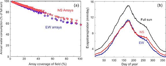
Figure 3. In panel (a), the cumulative annual water consumption predicted for agrivoltaic arrays in Tucson, AZ as a percentage of the full-sun annual evapotranspiration (ET) demand, versus the fraction of the field covered by the arrays in a top-down view. In panel (b), the daily evapotranspiration rate over the course of the year for agrivoltaic arrays with ∼50% coverage in Tucson, AZ. The North-South (NS) array has panels tilted 20 degrees to the west and the East-West (EW) array has panels tilted 30 degrees to the south.
Download figure:
Standard image High-resolution imageAgrivoltaic arrays with different azimuth orientation but equivalent coverage both decrease water consumption by a similar amount relative to the full sun baseline (figure 3(b)). The NS array has a higher water consumption in the winter months, while the EW array is higher in the early summer, suggesting seasonal variations in the shading pattern for the two classes of array.
The daily and seasonal trends in shading fraction for these two arrays (see supplemental) illuminate these seasonal differences in water consumption. For south-tilted EW array, the shade fraction is higher in winter months when the sun's average zenith angle is larger, but the shade fraction does not vary over the course of the day. By contrast, the NS array has a consistent shade fraction over the course of the year, but the tilt to the west causes a higher shade fraction in the afternoon, with most light reaching the ground in the morning. The shade fraction averaged over the day for a NS array is independent of the panel tilt angle, only the distribution of light within the day is affected.
3.2. Crop productivity results
For the sun-tolerant crop (figure 4(a)), productivity in the shade is lower than productivity in the sun for the entirety of both days considered. By contrast, the shade-tolerant model (figure 4(b)) shows lower in-shade productivity on day 50, but higher in-shade productivity the majority of day 200. On day 200, the temperature rapidly rises to a level above the peak activity temperature for the model in full-sun, and productivity is suppressed. In the shade, the model has a higher peak activity temperature and suffers a less severe mid-day depression in productivity. Over the course of the year, the shade-tolerant daily plant productivity in the agrivoltaic setting shows a large variation, ranging from 40% of the control productivity in the winter to over 110% of the control setting productivity for days in the mid to late summer. The sun-tolerant plant model also exhibits lower productivity in winter, particularly for EW arrays at roughly 50%–60% of the control setting, however in summer the productivity is only 80% of the control setting value for both EW and NS arrays.
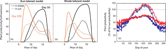
Figure 4. In panel (a), the plant productivity over the course of days 50 and 200 for plants in full sun and full shade based on a sun-tolerant plant model. In panel (b), the plant productivity over those days in full sun and full shade for a shade-tolerant plant model. In both (b) and (c), solid traces indicate full-sun conditions and dotted traces indicate full shade. The color of the trace indicates the day of year which supplied the temperature and illumination values for the plant model inputs.In panel (c), the total daily plant productivity as a percentage of the full sun productivity for both plant models under agrivoltaic arrays with 50% coverage in Tucson, AZ. The east-west oriented array traces are blue and the north-south traces in red. Solid curves indicate the sun-tolerant plant model and dotted curves correspond to the shade-tolerant model.
Download figure:
Standard image High-resolution imageComparing the performance of both crop models over the full year (figure 5(a)), as the field coverage fraction increases, plant productivity suffers a larger penalty relative to the control case. The shade-tolerant crop model shows a slightly higher crop productivity compared to the sun-tolerant model for arrays with NS rows. For field coverage fractions of 40% or higher, plant productivity varies by roughly 10 to 20 percentage points, depending on the combination of crop and array design.
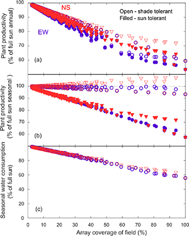
Figure 5. In panel (a), the cumulative annual plant productivity as a percentage of productivity in full sun for plants grown under agrivoltaic arrays relative to the coverage fraction of the array. In panel (b), the plant penalty vs the coverage fraction over the summer growing season (day 120 to day 275). In both panels, east-west array points are shaded blue, while north-south points are shaded red. Filled markers indicate the sun-tolerant plant model, while open markers indicate the shade-tolerant plant model. The dashed line at y = 100% is included to guide the eye. In panel (c), the water consumption over the summer growing season, as a percentage of the full sun water consumption, versus the field coverage. Again, East-West array points are drawn as blue circles and north-south points as red triangles and these relationships reflect Tucson, AZ.
Download figure:
Standard image High-resolution imageReanalysis for the summer growing season alone (figure 5(b)) shows a large separation in the behavior of the two plant models. The sun tolerant crop productivity still declines with array coverage, but the shade-tolerant crop under NS arrays with a western tilt has a productivity up to 8% higher than the full-sun baseline. This effect comes from the uneven distribution of shading over the course of the day for west-tilted NS arrays, which allows the shade-tolerant crop to take advantage of morning sun while temperatures are lower. The crop productivity curves (figure 4(b)) illustrate this behavior in detail. The shade tolerant crop under EW arrays shows a productivity penalty of 10% or less compared to the baseline, but it receives no net benefit from the shading.
The water consumption over the summer growing season (day 120–day 275) versus the field coverage fraction (figure 5(c)) is almost identical to the full-year trend (figure 3(a)). For both NS and EW arrays, water consumption declines by roughly 45% of the array coverage fraction. This indicates that for NS arrays with 40% or higher coverage, the agrivoltaic field would have 20%–45% water savings over the full-sun control depending on the coverage level, with productivity enhanced above the baseline for shade-tolerant crops (figure 5(b)).
3.3. Location comparison
For Tucson (figure 6(a)) the shade-tolerant crop model productivity and water saving trade-off is small to positive. However, for the sun-tolerant model, the water savings are close to the loss in crop performance regardless of design. In the results for Stockton (figure 6(b)) the shade-tolerant model performs well but does not show productivity benefits. Tilted NS arrays lose less than 5% relative to the baseline. This performance difference compared to Tucson is due to the cooler temperatures in Stockton, which also result in lower water savings. For Aurora, CO (figure 6(c)), the behavior of both crop models and both array orientations collapse into a single behavior trend. Based on these simulations, an agrivoltaic system in Aurora would suffer a plant productivity penalty of roughly two thirds of the water savings over the summer growing season regardless of the coverage level when compared to a full-sun field. The water savings are lowest for this location among the three, at roughly 1/3 of the coverage level. The effect of warmer or cooler temperatures under the array also depends on location, crop type and season considered. In Tucson warmer temperatures reduce summer shade tolerant crop productivity to a level comparable to that in Stockton, while crops benefit from warmer temperatures in Aurora (see supplemental).
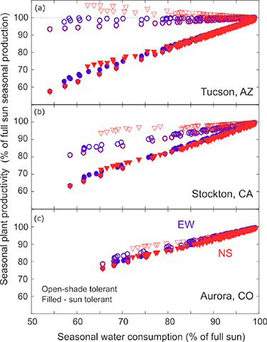
Figure 6. Plant productivity vs water consumption over the summer growing season (day 120 to day 275) for both shade-tolerant and sun-tolerant plant models at three locations. In panel (a), Tucson, AZ. In panel (b), Stockton, CA. In panel (c), Aurora, CO. In all panels, blue points correspond to East-West arrays, red to North-south, while filled markers indicate the sun-tolerant plant model and open markers indicate the shade-tolerant model. The dashed line at y = 100% in panel (a) is included to guide the eyes.
Download figure:
Standard image High-resolution image3.4. Land equivalent ratio analysis
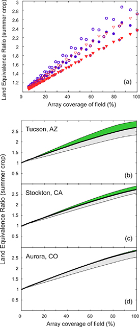
All agrivoltaic scenarios considered had LER values greater than one, indicating that even low-coverage designs increase the land use efficiency. While LER increases with area coverage, there is a large degree of variation in the LER at comparable coverage levels (figure 7(a)). At coverage of 60% and higher, the choice of array orientation and tilt and the shade tolerant vs sun tolerant crop can change the LER value by up to 0.6. In all cases, the range of potential LER values increases with the coverage, however the Aurora location LER values are much more closely bounded for a given coverage level. As the narrow green region indicates, this is due to the Aurora location having productivity independent of crop type (figure 7(c)).
Figure 7. In panel (a) the land equivalence ration (LER) vs area coverage for agrivoltaic arrays in Tucson, AZ including crop productivity over the summer growing season (day 120–day 275). In panels (b)–(d), the upper and lower bounds of LER vs area coverage for agrivoltaic systems in Tucson, AZ, Stockton, CA, and Aurora, CO. Portions of the plot shaded in green represent the amount of variation in LER controlled by crop selection. Portions shaded in gray represent the LER variation controlled by array design. The heavy black curve in the central region is the LER trend for arrays with sun-tolerant crops and EW arrays at 50% coverage and a 30 degree southern tilt, the baseline configuration.
Download figure:
Standard image High-resolution image
4. Discussion
Growing land-use conflicts between food and energy production have increased interest in agrivoltaics as a dual-use approach that could benefit both sectors. The design challenge of managing the tradeoffs associated with overstory PV panel light capture versus light transmission to food production has become a barrier to wider-scale adoption. Our modeling approach illustrates that agrivoltaics have potentially large benefits across the food, energy, and water sectors within drylands, such as the Southwestern US, but the benefits vary depending on the design of the agrivoltaic system. All locations examined showed a reduction in water consumption proportional to the array coverage level. This would represent a direct savings of irrigation inputs in a region with more than 8 million irrigated acres (Cody and Johnson 2015, Lahmers and Eden 2018) where the future water supply is projected to decline by 10%–20% on average (Pathak et al 2018, Sheikh and Stern 2019, Ray et al 2020, Miller et al 2021). We also illustrated multiple combinations of crop and array design minimally detrimental or even beneficial to crop productivity—even with array coverage exceeding 50%. These results indicate that tradeoffs between energy production and crop productivity are sensitive to local conditions. At the hottest, driest location, array design and crop selection combine to have large impacts on crop productivity. By contrast, at the coolest, wettest location, crop productivity varied only a small amount with crop type and array design. Finally, all locations showed the potential to have LER values of 2 or higher. PV developers have long been able to utilize a range of tools, such as the System Advisor Model, to anticipate electricity production within traditional PV systems (Blair et al 2018). This model provides a similar tool for predicting plant productivity in an agrivoltaic system, allowing stakeholders to quantify trade-offs to coupled food, energy, and water systems in their climate setting.
This new model identifies the role of array design in mediating the impact of the agrivoltaic array on crop productivity. Prior simulations of agrivoltaics that did not account for diurnal temperature variations have predicted that crop productivity would decline with array coverage (Dupraz et al 2011, Riaz et al 2020, Trommsdorff et al 2021), in contrast to experimental results (Barron-Gafford et al 2019). By including effects of temperature, the model can simulate crop productivity increases with coverage for specific array designs that create an uneven distribution of shading over the course of the day, with shading coinciding with high temperatures. This design approach results in shade-tolerant crop productivity up to 8% higher over the summer growing season than arrays with comparable coverage where the shade fraction does not vary over the course of the day and suggests that tracking arrays (ITRPV 2022) may further allow tailoring of the shade profile for maximum plant growth.
The second important insight from the model is the significance of crop selection. At the Tucson and Stockton locations, agrivoltaic shading is either minimally detrimental or positive for shade-tolerant plants. By contrast, sun-tolerant crops in this model respond to any shading with a loss of productivity proportional to the coverage level. The need to pair solar arrays with crop partners that tolerate shading has been well established (Dupraz et al 2011, Trommsdorff et al 2021, Riaz et al 2022), however this model gives insight into particular plant physiological characteristics that will perform well in agrivoltaic settings. Plants that are sensitive to high heat under high illumination conditions may benefit from agrivoltaic shading, particularly at hot locations. Our results are consistent with crop-specific models such as GECROS, which have predicted that agrivoltaics can increase unirrigated crop yields relative to full-sun controls in years with low precipitation (Amaducci et al 2018). Future research could modify these model functions with field-derived data on plant performance from specific crop types and any degree to which these crops can adapt to a shade. Photosynthetic acclimation—whereby leaves alter their morphology and/or biochemistry to adapt photosynthetic efficiency subject to long-term changes in the light environment—is well documented (Townsend et al 2018); however, no studies on plant acclimation within agrivoltaics exist to-date. Photosynthetic acclimation of crops in an agrivoltaics setting would likely increase the calculated benefits of agrivoltaics, and this represents a potentially valuable subfield of study.
The third fundamental characteristic considered in this study, geography, also governs the trade-offs between crop and energy in agrivoltaic systems. While all three locations saw a reduction in water consumption, the two hottest, driest locations showed a bifurcation in performance between shade and sun-tolerant crop types. At cooler, wetter Aurora, CO the model predicts no beneficial shading effects. Intriguingly, recent results from a nearby site showed that grasses growing beneath a photovoltaic array exhibited higher growth in regions receiving morning sun and afternoon shade despite having lower average soil moisture content than regions with morning shade and afternoon sun (Sturchio et al 2023). These experimental results suggest that (1) plants may acclimatize to agrivoltaic shading or (2) that the benefits of afternoon agrivoltaic shading may be more pronounced when crops experience water restriction. Both possibilities may be valid simultaneously.
The sensitivity of both water savings and crop productivity to the air temperature under the array (see supplemental) signals a need for more detailed modeling capturing the impact of the array on the local microclimate. Existing observations of array temperature impacts have focused on unirrigated dryland settings and a narrow range of array designs. A model that accounts for array design and density and predicts temperature effects on diurnal and seasonal time scales will be valuable for predicting array impacts on crop productivity.
The array, crop, and geographic drivers all affect LER. At all locations, the highest LER values at every coverage level were those that maximized electricity production rather than crop productivity. The west-tilted NS arrays that maximize crop production suffer a larger reduction in electricity production (∼10%) than the increase in crop productivity (at most 8%) relative to the comparable coverage EW array with a 30% tilt to the south. Within that context, the agrivoltaic system designer is presented with a trade-off: maximize crop production through afternoon shading at the expense of total electricity production. Similarly, a farmer seeking to reduce the irrigation demand of a shade-tolerant crop may choose to partner with an agrivoltaic array, thereby increasing the total system productivity with little or no crop productivity loss.
The results of this analysis suggest several avenues for further investigation to improve the fidelity and scope of subsequent crop models. Extending the plant model in this analysis to include performance under water stress would allow extension to settings dependent entirely on precipitation. Experiments aimed at identifying within-crop variability in traits linked with responses to environmental variability would facilitate tailored crop selection.
5. Conclusion
This analysis shows that integrated agrivoltaic systems have potential to benefit coupled energy, food and water systems by reducing land costs of photovoltaic production while maintaining agricultural production with lower water use. While the photovoltaic array can have a negative impact on crop productivity, all agrivoltaic systems considered had higher land use efficiency LER than equivalent conventional systems and reduced water consumption proportional to the coverage level. Agrivoltaic systems with roughly 50% coverage will reduce crop water consumption by 15%–20% or more depending on the location. Ultimately location, crop selection and array design combine to determine the agrivoltaics optimization landscape (Macknick et al 2022), and these results demonstrate the value of a modeling approach that captures agrivoltaic sensitivity to geography, crops, and array design.
This model allows system designers to quantify crop and energy tradeoffs for individual systems. For a given location and coverage the variation in LER depended on array design and crop selection choices. A system combining photovoltaics with a sun-tolerant crop or a system located in a climate similar to Aurora, CO, will face a direct tradeoff between energy production and crop productivity. If there is some maximum acceptable reduction in crop productivity for the farmer, that threshold will determine the maximum array density tolerable and consequently the maximum LER achievable by those systems. By contrast, in hot, dry locations with a shade-tolerant crop, productivity may in some cases increase with array coverage, thereby achieving a high LER with high density arrays. Maximizing crop production requires an array design that provides predominantly afternoon shading over a shade tolerant crop. This array orientation reduces electricity production 10%, but crop production remains high under very high coverage levels. In meeting the land needs for photovoltaic energy generation and ongoing investments in agriculture, agrivoltaics may provide benefits whose performance reflects geographically variability, array design choices, and crop performance.
Acknowledgments
This research received funding support from (1) the National Science Foundation Geography and Spatial Sciences through Award 2025727 and (2) the National Renewable Energy Laboratory's InSPIRE project, through the U.S. Department of Energy Office of Energy Efficiency and Renewable Energy (EERE) Solar Energy Technologies Office under award DE-EE00034165
Data availability statement
All data that support the findings of this study are included within the article (and any supplementary files).
Supplementary data (0.6 MB PDF)