


Abstract
We explore and evaluate various processes that could drive the variations in the volume mixing ratio (VMR) of atmospheric O2 observed by the quadrupole mass spectrometer (QMS) of the Sample Analysis at Mars (SAM) instrument suite on the Mars Science Laboratory (MSL) Curiosity rover. First reported by Trainer et al. (2019), these ∼20% variations in the O2 VMR on a seasonal timescale over Mars Years 31–34, in excess of circulation and transport effects driven by the seasonal condensation and sublimation of CO2 at the poles, are significantly shorter than the modeled O2 photochemical lifetime. While there remains significant uncertainty about the various processes we investigated (atmospheric photochemistry, surface oxychlorines and H2O2, dissolution from brines, and airborne dust), the most plausible driver is surface oxychlorines, exchanging O2 with the atmosphere through decomposition by solar ultraviolet and regeneration via O3. A decrease in O3 from increased atmospheric H2O would reduce the removal rate of O2 from the atmosphere to form oxychlorines at the surface. This is consistent with the tentative observation that increases in O2 are associated with increases in water vapor. A lack of correlation with the local surface geology along Curiosity's traverse within Gale crater, the nonuniqueness of the relevant processes to Gale crater, and the short mixing timescales of the atmosphere all suggest that the O2 variations are a regional, or even global, phenomenon. Nonetheless, further laboratory experiments and modeling are required to accurately scale the laboratory-measured rates to Martian conditions and to fully elucidate the driving mechanisms.
Export citation and abstract BibTeX RIS

Original content from this work may be used under the terms of the Creative Commons Attribution 4.0 licence. Any further distribution of this work must maintain attribution to the author(s) and the title of the work, journal citation and DOI.
1. Introduction
The Martian atmosphere is primarily composed of CO2 at 95%, with the remainder made up of minor species such as N2, Ar, and O2. Among these minor species, O2 has received particular and enduring scientific interest. Indeed, O2 is a key species behind one of the earliest problems in Mars science. Commonly referred to as the "stability of the Martian atmosphere," this problem suggests that the Martian CO2 atmosphere would gradually be converted into O2 and CO via photochemistry, resulting in the accumulation of large amounts of O2 and CO. However, the first characterizations of the Martian atmosphere in the 1960s using Earth-based spectroscopy (Chamberlain & Hunten 1965; Belton & Hunten 1966; Spinrad et al. 1966) and Mariner 4 radio occultation (Kliore et al. 1965; Chamberlain & McElroy 1966) found significantly less O2 and CO. While the classic papers of McElroy & Donahue (1972) and Parkinson & Hunten (1977) have supplied a key piece of the puzzle in the form of odd-hydrogen (HOx ) chemistry that is driven by species such as OH and HO2, the puzzle remains incomplete and discrepancies between models and observations still remain (Lefèvre & Krasnopolsky 2017). A highly reactive chemical species, O2 would also have played an important role in controlling chemical alteration rates at the surface and subsurface over the planet's history (e.g., Huguenin 1976; Burns & Fisher 1993; Lammer et al. 2003; Zolotov & Shock 2005; Zolotov & Mironenko 2007). This chemical reactivity of O2 also makes it an important metabolite for complex life, and the O2 partial pressure (pO2) is often a crucial parameter in discussions of the astrobiological potential of an environment and the metabolic pathways it can support (e.g., Rummel et al. 2014).
O2 in the Martian atmosphere has been measured via a variety of observational techniques and geometries. Earth-based spectroscopic measurements include early telescopic observations by Barker (1972), Carleton & Traub (1972), and Trauger & Lunine (1983), as well as more recently by Hartogh et al. (2010). At Mars, O2 has been measured in stellar occultations by both the SPectroscopy for the Investigation of the Characteristics of the Atmosphere of Mars (SPICAM) on Mars Express (Sandel et al. 2015) and the Imaging UltraViolet Spectrograph (IUVS) on the Mars Atmosphere and Volatile EvolutioN (MAVEN) spacecraft (Gröller et al. 2018). In situ measurements have been made by the Viking mass spectrometers in the atmosphere (Nier & McElroy 1977) and on the surface (Owen et al. 1977), as well as by the Sample Analysis at Mars (SAM) on the Curiosity rover of the Mars Science Laboratory (MSL) mission (Trainer et al. 2019). These measurements have generally returned O2 volume mixing ratios (VMRs) on the order of 10−3. While differences across the data sets could simply be due to the different instrument calibrations, the O2 VMR is also found to vary within individual data sets, indicating that these variations are physically real. In particular, the SAM observations show seasonal variations of as much as 20% over the small region in Gale crater where the Curiosity rover has been traversing (Trainer et al. 2019). With O2 having a photochemical equilibrium lifetime of ∼60 yr (Krasnopolsky 2017), variations of this magnitude over a timescale of 100 sols are unexpected.
In this paper, we will be exploring potential abiotic drivers behind the variations in O2 VMR observed by SAM at Gale crater, in particular the unexpected rise of O2 over the first half of the Martian year followed by its equally unexpected decline afterward. We will first introduce the data set in the next section, before evaluating the potential drivers from atmospheric photochemistry and surface processes in Section 3. In Section 4, we look at some factors that are potentially correlated with the observations and their implications. We conclude in Section 5.
2. MSL SAM O2 VMR Observations
The Quadrupole Mass Spectrometer (QMS) in the SAM instrument suite on the MSL Curiosity rover conducts periodic sampling and measurement of the VMRs of the five most abundant species—CO2, N2, Ar, O2, and CO—in the ambient atmosphere around the rover. This experiment has been described extensively in Mahaffy et al. (2012) and Franz et al. (2014). Briefly, the gas manifolds in the instrument are first evacuated and the background signal is measured. Then, an atmospheric sample is ingested into the instrument through an inlet valve that subsequently closes to isolate the sample from the Martian environment. This sample is introduced through a glass capillary inlet into the QMS ion source, where it is ionized via electron ionization by a filament. A combination of radio frequency and static voltages is applied to four hyperbolic rods to achieve mass separation in the mass analyzer, and the counts are measured at intervals of 1 ("unit scan") or 0.1 ("fractional scan") in the mass-to-charge ratio (m/z, with m given in daltons 5 and z in terms of the elementary charge e). After background subtraction (Trainer et al. 2019), the quantities of CO2, N2, O2, and CO relative to 40Ar are determined through the application of calibration constants and secondary correction factors to the measured counts for their respective "marker" fragments relative to the measured count for m/z = 40, the marker fragment for 40Ar (Franz et al. 2015, 2017). For O2, the marker fragment is the molecular ion at m/z = 32. The VMRs of the five species are then calculated by renormalizing their relative quantities such that they now sum to unity. Absolute quantities (such as partial pressures) of the five species are not measured by SAM, although the Rover Environmental Monitoring Station (REMS) on Curiosity does measure surface pressures (Gómez-Elvira et al. 2012).
Over the observation period spanning Mars Years (MY) 31–34, the O2 VMR was found to exhibit significant variation (Trainer et al. 2019). These O2 VMR measurements are reproduced in Appendix A. As noted in Trainer et al. (2019), very high signal levels were seen in the instrument during the first full derivatization experiment on the Ogunquit Beach (OG) dune sample on sol 1909 (Malespin et al. 2018). This experiment on sol 1909 (2017 December 19) caused a shift in the sensitivity of the instrument detector, requiring a change in the QMS electron multiplier gain setting and reevaluation of the calibration constants. Thus, while more VMR measurements have been taken since sol 1909 (Appendix E), these measurements will be presented and discussed in a future work, pending confirmation of the new calibration constants. Here we focus on interpretation of the O2 variability described in Trainer et al. (2019).
These VMR variations are the sum of effects from a variety of phenomena, which we shall divide into two classes. The first class comprises circulation, transport, and mixing processes that do not change the total amount of O2 in the atmosphere. In the lower atmosphere (<∼80 km) that is sampled by Curiosity, mean meridional circulation and transport around the equinoxes resemble classic Hadley circulation in Earth's troposphere, with ascending branches near the equator and descending branches ∼30° away (Barnes et al. 2017). These vertical branches are connected by horizontal branches, which bring polar air to the equatorial regions near the surface and equatorial air to the polar regions at altitude. However, differences between Mars and Earth translate into deviations from this classic picture over the rest of the year. The low surface thermal inertia of Mars results in larger temperature variations at the higher latitudes with the seasons. Furthermore, the thinness of the Martian atmosphere means that CO2 condensation and sublimation at the polar regions can give rise to significant surface pressure changes, such as a 30% decrease during southern winter (e.g., Hess et al. 1980). The result is a striking dominance of one of the Hadley cells over the other, with the dominant cell spanning both sides of the equator with a width of more than 90° of latitude. This puts the ascending branch in the warmer/summer hemisphere and the descending branch in the cooler/winter hemisphere, with horizontal transport near the surface from the latter to the former.
The VMR of O2 and other minor atmospheric species is affected by the aforedescribed circulation and transport. In addition, there is also mixing arising from the change of atmospheric composition from CO2 freezing onto and subliming from the polar regions. We can trace the sum of these effects through the VMR of another minor species, the noncondensible and inert Ar. In the equatorial region where Curiosity is, the Ar VMR has been observed to vary seasonally by ∼10% with the Mars Odyssey Gamma Ray Spectrometer (GRS; Sprague et al. 2012), MSL SAM (Trainer et al. 2019), and the Alpha Particle X-ray Spectrometers (APXS) on the Mars Exploration Rovers (MERs) and MSL (VanBommel et al. 2018, 2020). Over southern fall and early winter, "freeze distillation" from CO2 freezing out onto the south polar cap results in an enrichment of Ar in the air mass over the pole, reaching a maximum at LS ∼ 120° (Lian et al. 2012; Sprague et al. 2012). Mixing of this enriched air mass with the lower latitudes is hampered by the strong polar vortex, however. At LS ∼ 150°, net accumulation of CO2 ice onto the polar cap switches to net sublimation, and dilution starts to occur instead of enrichment. This dilution reduces the Ar VMR directly over the polar cap, creating a front enriched in Ar at the boundary of the polar vortex. The increasing pressure from CO2 sublimation also weakens the polar vortex and pushes the enriched front northward along the lower horizontal branch of the Hadley circulation. This gives rise to the maximum in Ar VMR at LS ∼ 210° preceding the maximum in surface pressure at LS ∼ 250° at the equatorial region, an observation made by the MERs (VanBommel et al. 2018, 2020) and MSL (Trainer et al. 2019). The Ar VMR continues to fall with further CO2 sublimation and transport from the south pole. A similar and complementary phenomenon occurs over the north polar region, with a smaller maximum in northern spring compared to that in southern spring due to a weaker polar vortex from the proximity of northern winter with perihelion. These effects are expected to act on the other noncondensible species in the atmosphere to a similar degree to that on Ar—indeed, SAM has observed the N2 VMR to vary seasonally in the same way as the Ar VMR (Trainer et al. 2019).
In addition to the mean circulation, thermal tides and planetary waves can arise from perturbations in the atmosphere (such as from the differential heating of the surface by solar radiation) and manifest as oscillations in atmospheric temperature, pressure, and density (Forbes et al. 2002) with periods ranging from less than a sol to several sols. These phenomena and their effects on the local circulation at Gale crater have been well documented (e.g., Haberle et al. 2014; Guzewich et al. 2016; Martínez et al. 2017; Viúdez-Moreiras et al. 2020a; Battalio et al. 2022). Similar to transport and mixing processes, tides and waves do not change the total amount of noncondensible species in the atmosphere. Instead, their effects act on the entire volume of the local atmosphere and thus can be tracked by inert tracers such as Ar. Over the duration of sols 45–1869 that is spanned by our data set, Curiosity's elevation has also varied between −4521 and −4172 m relative to the aeroid from its traverse over the bottom of Gale crater. While these elevation changes have an effect on the measured surface pressures (Martínez et al. 2017), the atmosphere is well mixed at these elevations, and they should not have a significant effect on the measured VMRs.
The abovementioned processes have similar effects on O2 to those they have on Ar, and we can remove the sum of their effects and isolate any residual variations in the O2 VMR by normalizing the O2 VMR by the Ar VMR. In contrast to Trainer et al. (2019), where the O2 VMR was normalized through dividing by the absolute Ar VMR, here we choose a different method that will preserve useful information about the absolute magnitudes of the O2 VMR variations. We first divide each Ar VMR measurement by the mean of all the Ar VMR measurements to determine the relative Ar variation. Each O2 VMR measurement is then normalized by dividing by the relative Ar variation that corresponds to the same TID as the O2 measurement. Figure 1 shows the O2 VMR after this normalization procedure. We can see that there are residual variations of as much as ±400 ppmv or 20% in the O2 VMR that cannot be attributed solely to the "bulk redistribution" processes described above that would effect VMR changes in all the noncondensible minor species collectively. Instead, these residual O2 VMR changes will be due to O2-specific processes that change the amount of O2 in the atmosphere. The second class of processes involving the addition or removal of O2 from the atmosphere will be the focus for this paper.

Figure 1. O2 VMR against LS over MY 31–34, normalized by the fractional variation of 40Ar VMR measurements about their mean. The gray line indicates the mean value. The increases in normalized O2 VMR at the beginning of MY 32, 33, and 34 are highlighted with dashed lines, with their different slopes from possible interannual variability.
Download figure:
Standard image High-resolution image3. Evaluating Potential O2 Sources and Sinks
Figure 1 shows the variation in the O2 VMR that we attribute to O2-specific processes after removing the contribution from bulk redistribution processes that is represented in the Ar VMR. Over the first half of the Martian year, we see increases of ∼300 ppmv in the normalized O2 VMR, indicating addition of O2 into the atmosphere. There are also decreases (most notably the ∼400 ppmv drop occurring at LS ∼ 150° in MY 33), indicating O2 removal. There appears to be noticeable interannual variability in terms of the magnitude and timing of the increases.
In this study, we will explore and evaluate the possible drivers behind these increases and decreases in the normalized O2 VMR. For this, we adopt the strategy of looking for oxygen 6 reservoirs of sufficient size and processes that can exchange O2 between these reservoirs and the atmospheric O2 reservoir at a sufficient rate. To do this, we have to convert the variations in the normalized O2 VMR to requirements on the number density and rate. Over a Martian year at Gale, the daily mean near-surface air temperature ranges between 210 and 235 K, while the daily mean near-surface atmospheric pressure varies between 740 and 920 Pa (Martínez et al. 2017). Estimating using the ideal gas law, we get a near-surface total number density of (2–3) × 1017 cm−3. Using the normalized O2 VMR values, this translates into the requirement of 1014 O2 molecules cm−3 for the minimum reservoir size. The increases and decreases occur over a timescale of ∼100 sols (107 s), and this gives us the requirement of a minimum exchange rate of 107 O2 molecules cm−3 s−1.
Since our discussion is about atmospheric O2, it will be natural for us to start our search with the other oxygen reservoirs in the atmosphere. Oxygen in these reservoirs would be converted to and from O2 through atmospheric photochemistry.
3.1. Atmospheric Photochemistry
Atmospheric photochemistry comprises the set of chemical reactions involving atmospheric species that is primarily driven by solar radiation. Generally, atmospheric photochemistry at Mars tends not to be spatially localized. The photochemistry that occurs at some local volume of the atmosphere would be determined by the composition and temperature of the volume, as well as the incident solar radiation flux. All these quantities vary gradually over the Mars atmosphere, mediated by the relatively short transport and mixing timescales. Simulations using global circulation models (GCMs) found both the vertical and horizontal mixing timescales to be less than 100 sols (e.g., Barnes et al. 1996), except over the polar regions at altitudes 20–40 km, where the timescales can be higher than 200 sols (Waugh et al. 2019). Given Curiosity's location in Gale crater at −5° N, these air masses, restricted by the polar vortex, would not have a significant influence on the ambient atmosphere around Curiosity and thus are not relevant to this study. Although the relief of ∼6 km at Gale crater has some effects on the local atmospheric circulation (e.g., Rafkin et al. 2016), the high eddy diffusivities up to 107 cm2 s−1 (e.g., Taylor et al. 2007; Pathak et al. 2009) and the growth of the planetary boundary layer to several kilometers in the daytime (Guzewich et al. 2017; Fonseca et al. 2018) would have facilitated mixing of the atmosphere between the inside and outside of the crater. Modeling of the circulation within the crater also found fast mixing timescales of 1 sol (Pla-García et al. 2019). With the transport and mixing timescales being shorter than the 100 sol timescale of the O2 variations, the O2 variations observed by Curiosity at Gale crater and any photochemical process driving them are likely not localized to Gale crater, but rather part of a larger global phenomenon.
With this assumption, we use a 1D globally averaged coupled ion–neutral photochemical model to investigate oxygen photochemistry in the Martian atmosphere. The details for this model have previously been described in Lo et al. (2021). Spanning the surface to 240 km altitude at a resolution of 1 km, this model calculates the number densities of the various species and the rates of the various reactions at steady state using an exhaustive reaction list with the most updated reaction rates and cross sections, making it well suited for a comprehensive investigation of the effects of photochemistry on the surface O2 VMR. While the use of a 1D photochemical model offers efficiency in our search for any potentially important but previously ignored reaction in its exhaustive reaction list and our investigation into the effect of different boundary conditions (Section 3.2), many phenomena that are relevant and important to our problem cannot be modeled by a 1D photochemical model. To mitigate these limitations, we use average temperatures and number densities of CO2, N2, Ar, and H2O from the Mars Climate Database (MCD, version 5.3) at different seasons and solar activity levels for our model inputs. The MCD is a collection of results from the Mars Planetary Climate Model (PCM), developed at the Laboratoire de météorologie dynamique (LMD) of the French Centre national de la recherche scientifique (CNRS) (Forget et al. 1999; Millour et al. 2018). Results from the MCD have been extensively validated using available observational data and span the altitude range of the photochemical model, allowing for ease of its incorporation as inputs. Separate temperature and number density profiles are constructed for different seasons and solar activity levels. For seasons, a set of aphelion profiles based on MCD results from LS = 60° to 90° (aphelion occurs at LS = 71°) and a set of perihelion profiles based on MCD results from LS = 180° to 330° are constructed to account for the dependence of the photochemical processes on the highly varying solar radiation flux from the eccentricity of the Martian orbit. The different solar activity levels are set through the MCD "solar maximum" and "solar minimum" climatology scenarios. In addition to being able to describe 3D circulation, the PCM models a wide variety of phenomena not in the photochemical model, such as dust and ice aerosols, CO2 ice formation and sublimation on the ground and in the atmosphere, and the water cycle with modeling of cloud microphysics. These phenomena are key to an accurate description of the temperatures and H2O abundance, important variables for controlling oxygen photochemistry.
Figure 2 shows the main reactions that make up oxygen photochemistry at Mars, as elucidated from the photochemical model. Although we have included a maximal set of oxygen reactions available in the literature in our photochemical model, many of these reactions have turned out to be insignificant, and the overall picture we obtained is consistent with previous results from other photochemical models (e.g., Atreya & Gu 1995; Krasnopolsky 2010; Viúdez-Moreiras et al. 2020b). Ultimately, O2 is sourced from the photodissociation of CO2 and H2O by solar ultraviolet (UV) radiation. Based on the model, the highest rates for O2 production come from seven reactions:


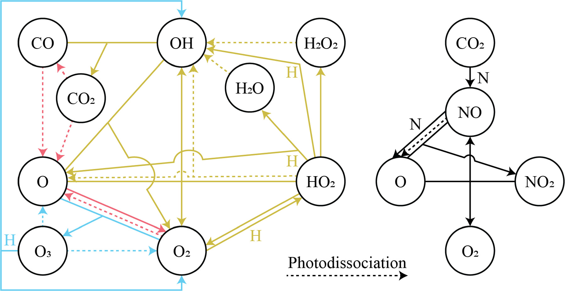
Figure 2. Schematic of significant species and reactions for oxygen photochemistry in the Martian atmosphere. For clarity, the reactions are divided into those involving COx and HOx on the left and those involving NOx on the right. Arrows point from reactants to products, with dashed lines indicating photodissociation reactions. "H" or "N" indicates a reaction with atomic hydrogen or atomic nitrogen, respectively, while the third bodies ("M") for carrying away momentum in three-body reactions are not shown. Colors indicate the reaction groups as discussed in the text: red for "CO2 photodissociation," yellow for "HOx chemistry," blue for "O3 photochemistry," and black for "NOx chemistry."
Download figure:
Standard image High-resolution imageHere M represents a third body, typically CO2 at Mars, required for the conservation of momentum in the reaction. The majority of O2 loss occurs via three reactions:


Rate coefficients for the above reactions are provided in Table B1 in Appendix B. For ease of discussion, we classify the seven production reactions and three loss reactions into four groups. The first group, which we shall refer to as "CO2 photodissociation," comprises reactions (P1) and (L1). The second group of "HOx chemistry" comprises (P2), (P3), (P4), and (L2), and the third group of "NOx chemistry" comprises (P5). The fourth group of "O3 photochemistry" comprises (P6), (P7), and (L3).
The first group of "CO2 photodissociation" is so named because it comprises the channel for the formation of O2 from CO2. O is primarily produced from the photodissociation of CO2, either directly or through a two-step process involving CO. This O is then rapidly converted into O2 through (P1), with the reverse reaction of (L1) maintaining a small amount of O and preventing O2 from increasing indefinitely. These two reactions of (P1) and (L1), together with the CO2 photodissociation reaction, are among the oldest known reactions in the Martian atmosphere, and they set the stage for the scientific problem of the "stability of the Martian atmosphere." The fast (P1) versus the slow spin-forbidden CO + O + M → CO2 + M (reaction constants k at 200 K of ∼10−33 cm6 molecule−2 s−1 and ∼10−36 cm6 molecule−2 s−1, respectively; Tsang & Hampson 1986) would result in the accumulation of substantial CO and O2 in the atmosphere, and at a ratio of 2:1.
The observed quantities of CO and O2 at Mars are 2 orders of magnitude smaller than predicted by the "CO2 photodissociation" reactions alone, and in a 1:2 ratio rather than the predicted 2:1. The "HOx chemistry" reactions were proposed as a solution. Sourced from the photodissociation of H2O, the HOx species (H, OH, and HO2) form two catalytic cycles regenerating CO2 from CO, O, and O2. The first cycle, proposed by McElroy & Donahue (1972), comprises


with the net effect of converting CO and O into CO2. The second cycle, proposed by Parkinson & Hunten (1972), comprises


with the net effect of converting CO and O2 into CO2.
From the perspective of O2, HOx chemistry introduces H2O as a second ultimate source of O2 through (P2), with a column-integrated rate ∼85% that of (P1) at aphelion and a much larger 7–8 times that of (P1) at perihelion when the H2O abundance is significantly higher. The first cycle, with 10 times the rate of the second cycle (e.g., Nair et al. 1994; Krasnopolsky 2010), is net neutral with respect to O2. Net O2 loss with the breaking of the O–O bond can occur through the second cycle with H2O2 photodissociation, or earlier with HO2 photodissociation or reaction with H after its primary production reaction of (L2). Collectively, these three reactions make up ∼30% of the breaking of the O–O bond, while (L1) makes up ∼50% (Lefèvre & Krasnopolsky 2017). The dominance of (P3) over (P4) also results in the preferential consumption of O over O2, tipping the equilibrium CO:O2 ratio toward higher O2 .
NOx chemistry comprises a cycle converting O into O2 through reaction with NO and NO2. NO, produced from the reaction of CO2 with N (produced from N2 photodissociation at ∼120 km), first reacts with O to form NO2, and further reaction of NO2 with O produces O2 and regenerates NO through (P5). The column-integrated rate for (P5) is about 30% that of (P2) during the perihelion season, and about 10% during aphelion. NO2 can also be produced from reaction of NO with HO2 (this constitutes the remaining ∼20% of O–O bond breaking; Lefèvre & Krasnopolsky 2017), but with the subsequent production of O2 through (P5) there is no net O2 loss through this channel.
Finally, O3 photochemistry comprises the rapid interconversion between O2 + O and O3 via (P6) and (L3) and conversion of O3 back into O2 with OH through (P7). All these reactions preserve the O–O bond and are together net neutral with regard to O2. As a result of this and the significantly higher rate of (P6) and (L3) over the other O2 formation and loss reactions, we can effectively treat each O3 molecule as the combination of an O2 molecule and an O atom for the purposes of bookkeeping the O2 in the Martian atmosphere.
Understanding how the various O-containing species are linked to O2 through photochemical reactions allows us to examine the photochemical drivers behind the observed O2 variations. From the VMRs of the various O-containing species provided in Table 1, we find that only CO2, CO, and H2O have sufficiently high VMRs to function as potential oxygen reservoirs for driving the O2 variations. An important point to note is that although the atmospheric H2O reservoir has a maximum VMR of only 200 ppmv, there is significant exchange with the surface H2O reservoirs, and thus the amount of available oxygen can actually be higher. Indeed, sublimation and condensation of frost at the higher latitudes (particularly the north polar cap) are a significant driver for variations of atmospheric H2O on the seasonal timescale (e.g., Montmessin et al. 2017). This is handled in the photochemical model through fixing the H2O number density profile, such that the atmospheric H2O reservoir is never depleted and the steady-state number densities and reaction rates are calculated based on this fixed density profile. For O, even though it has a somewhat high VMR at 135 km altitude, it is important to remember that the overall density of the atmosphere decreases with altitude. Taking into account the difference in pressures between 135 km and the surface, the actual amount of O from 135 km will correspond to a much smaller (and insufficient) VMR if brought down to the surface. This is also reflected in the lower column-averaged VMR, which is strongly weighted toward the surface in its calculation. While the abundances of O, OH, HO2, H2O2, NO, and NO2 are too low for them to function as oxygen reservoirs, these trace species can act as bridges connecting O2 to the CO2, CO, and H2O reservoirs.
Table 1. Volume Mixing Ratios of the O-containing Species in Figure 2
| Species | VMR | Altitude | Reference |
|---|---|---|---|
| CO2 | 0.945–0.954 | surface | Trainer et al. (2019) |
| CO | 400–1200 ppmv | surface | Trainer et al. (2019) |
| 400–2000 ppmv | 0–60 km, outside poles | Olsen et al. (2021a); Fedorova et al. (2022) | |
| 400–4000 ppmv | 0–60 km, including poles | Olsen et al. (2021a); Fedorova et al. (2022) | |
| H2O | 0–30 pr. μm | column | Smith et al. (2009); Crismani et al. (2021) |
| 0–200 ppmv | 0–100 km | Fedorova et al. (2023) | |
| O | 0.5–0.7 ppmv | column average | this study |
| 0.5–1.2% | 135 km | Strickland et al. (1972); Chaufray et al. (2009) | |
| O3 | 0–30 μm atm | column | Lefèvre et al. (2021) |
| 0–800 ppbv | 0–30 km | Olsen et al. (2022) | |
| OH | 10−12 | column average | this study |
| 10−11–10−10 | peak at ∼30 km | this study | |
| HO2 | 10−12–10−11 | column average | this study |
| 10−11–10−10 | peak at 20–30 km | this study | |
| H2O2 | 0–40 ppbv | column average | Clancy et al. (2004); Encrenaz et al. (2004, 2015) |
| NO | 10−9 | column average | this study |
| 10−5–10−4 | 120–140 km | Nier & McElroy (1977); Stevens et al. (2019); Cui et al. (2020) | |
| NO2 | 10−12 | column average | this study |
| 10−12–10−9 | peak at 160–190 km | this study |
Note. Provided are the column-averaged values, representing the total amount of the species in the atmosphere, and the values at specific altitudes of interest. Derived from Lefèvre & Krasnopolsky (2017).
Download table as: ASCIITypeset image
Even if the CO2, CO, and H2O reservoirs contain more oxygen than the O2 variations, not all the oxygen in these reservoirs will be liberated to eventually form O2. From Figure 2, we can see that photodissociation is the key gatekeeper step in the conversion of CO2, CO, and H2O into O2, with O and OH functioning as intermediaries. Since the observed O2 variations are deviations from an equilibrium VMR of ∼1700 ppmv, it would be the variations in the photodissociation rates over time, rather than the total rates, that would provide the additional release of oxygen to drive O2 increases above its equilibrium value.
Photodissociation of CO2 can produce O in the ground (3 P) or excited (1 D) state, with the combined rate peaking at ∼30 km altitude in our dust-free photochemical model. The preponderance of CO2 in the atmosphere means that CO2 photodissociation rates depend mostly on the solar UV flux, and thus the 40% increase in solar UV flux from aphelion to perihelion translates into a comparable increase of 50% in the column-integrated rate (Table 2). High solar activity also increases rates by about 10% compared to low solar activity. If we assume the CO2 photodissociation rate to vary sinusoidally over the Martian year between the maximum and minimum values for each solar activity scenario and all liberated O from this variation to be immediately converted into O2, we will find O2 variations with a column-integrated amplitude of ∼4 × 10¹⁸ O2 molecules cm−2 for both solar activity scenarios. If we further assume that these variations are well mixed down from the photodissociation peak at 30 km to the surface with a 10 km scale height, then we would get an increase of ∼4 × 10¹² molecules cm−3 in the surface O2 number density. Even with the two preceding assumptions that would maximize the variations in surface O2, we get a value that is more than an order of magnitude smaller than our requirement of 1014 molecules cm−3.
Table 2. Modeled Column-integrated Rates for Selected Reactions from Figure 2
| Column-integrated Rate (cm−2 s−1) | ||||
|---|---|---|---|---|
| Reaction | Perihelion, LSA | Aphelion, LSA | Perihelion, HSA | Aphelion, HSA |
| CO2 + h ν → CO + O | 1.2 × 10¹² | 8.1 × 10¹¹ | 1.3 × 10¹² | 9.0 × 10¹¹ |
| CO + h ν → C + O | 1.6 × 10⁷ | 8.7 × 10⁶ | 6.0 × 10⁷ | 3.0 × 10⁷ |
| H2O + h ν → OH + H | 6.1 × 10⁹ | 7.6 × 10⁷ | 6.8 × 10⁹ | 8.4 × 10⁷ |
| O2 + h ν → 2O | 3.2 × 10¹⁰ | 1.7 × 10¹⁰ | 3.7 × 10¹⁰ | 2.0 × 10¹⁰ |
| HO2 + h ν → OH + O | 8.2 × 10⁸ | 6.2 × 10⁷ | 9.3 × 10⁸ | 7.0 × 10⁷ |
| HO2 + H → 2OH | 5.2 × 10¹⁰ | 5.4 × 10⁸ | 6.0 × 10¹⁰ | 6.2 × 10⁸ |
| HO2 + H → H2O + O | 1.2 × 10⁹ | 1.2 × 10⁷ | 1.3 × 10⁹ | 1.4 × 10⁷ |
| H2O2 + h ν → 2OH | 2.3 × 10⁷ | 4.8 × 10⁵ | 2.8 × 10⁷ | 5.6 × 10⁵ |
Note. Products include both ground and excited states. LSA: low solar activity; HSA: high solar activity.
Download table as: ASCIITypeset image
Photodissociation of CO occurs high in the atmosphere, with rates peaking at ∼140 km altitude and dropping to zero below 90 km. Overall rates and their variation with season are much lower compared to CO2 photodissociation (Table 2). Applying the same treatment as in CO2 photodissociation, we find that increased CO photodissociation rates can only give rise to a very small increase of 108 molecules cm−3 in O2 surface number density, making it unlikely that CO photodissociation would play a significant role in driving the observed O2 variations.
With a peak at ∼50 km altitude, H2O photodissociation rates vary significantly with the seasons (Table 2), driven by the highly varying H2O abundance (Table 1) arising from exchange with the surface reservoirs. Nonetheless, these seasonal variations are not sufficient, providing an increase of only 1011 molecules cm−3 in the surface O2 number density under the two maximalist assumptions.
Just as variations in the photodissociation rates of CO2, CO, and H2O could drive O2 variations by controlling the release of oxygen, variations in the rates of the various O2 loss processes can do the same by taking O2 out of the atmosphere. Ultimate loss of O2 occurs through O2 photodissociation into O in (L1) and the loss of HO2 after (L2). While most HO2 is regenerated into O2 through (P3), a fraction is lost through photodissociation, reaction with itself ((P4), followed by photodissociation of the H2O2 product), and reaction with H.
O2 photodissociation occurs primarily at the surface. Seasonal variations in its rate are too small, translating to a variation of only 1011 molecules cm−3 under the two assumptions.
The HO2 loss reactions of photodissociation and reaction with H both peak at 20–30 km altitude, driven primarily by the HO2 density peak there. We find that the maximum O2 variation from HO2 photodissociation is 1010 molecules cm−3, while those from reaction with H to form OH and to form H2O and O are 1012 and 1010 molecules cm−3, respectively. HO2 can also react with itself to form H2O2, which then photodissociates with a peak rate also at 20–30 km altitude. Maximum seasonal variation from this channel corresponds to 108 molecules cm−3.
Altogether, the seasonal variability of the production and loss channels can only account for O2 variations that are an order of magnitude smaller than observed. In addition to the maximalist assumptions that all liberated O is converted into O2 and the O2 variations are confined to the bottom 10 km of the atmosphere, the photodissociation rates above are calculated assuming an aerosol-free atmosphere. In reality, aerosols from dust and condensates can increase atmospheric UV opacities, reducing photodissociation rates. This effect is particularly significant below ∼40 km altitude and is stronger during the perihelion season (e.g., Montmessin et al. 2006; Määttänen et al. 2013), thus countering the increase in the solar UV flux then. The UVISMART radiative transfer model, which includes these aerosol effects and has also been validated with in situ data from Curiosity, found that UV irradiance at Gale crater generally varies throughout the year within a band of ±15% (Viúdez-Moreiras 2021), smaller than the 40% used in the photochemical model. With their peak rates occurring within the aerosol haze layer, photodissociation of CO2, O2, HO2, and H2O2 would be significantly affected by the inclusion of aerosol effects. Their rates would vary less with the seasons, making them even less viable drivers for the observed amplitudes in the O2 variations.
Thus, even though there are oxygen reservoirs in the Martian atmosphere with sizes larger than the magnitude of the O2 variations, the processes linking these reservoirs to O2 do not vary enough to produce sufficiently large variations about the equilibrium O2 VMR in the required time frame. The O2 variations cannot be driven by atmospheric photochemistry alone, and we need to look toward surface processes for an answer.
Before we do so, however, a caveat has to be noted. The photochemical stability of the Martian atmosphere is still not well understood today, and this poor understanding shows up as very low modeled values for long-term equilibrium CO and O2 VMRs. A common "solution" for the low O2 VMRs in 1D photochemical models is to introduce a surface flux through the lower boundary condition, either directly with an appropriate magnitude to match the observations or indirectly by setting the abundance (e.g., Atreya & Gu 1995). This O2 surface flux seems plausible, but justification has generally been poor in the instances where it has been invoked. We will examine the processes that can contribute to this surface flux later in Section 3.2. The same is not plausible for CO, however, giving rise to the "CO problem," where modeled CO VMRs are as much as 7 times lower than the observations. Lefèvre & Krasnopolsky (2017) provides an excellent exposition of the problem. GCMs with photochemistry, such as PCM (Forget et al. 1999) and GEM-Mars (Neary & Daerden 2018), generally avoid the O2 and CO problems by picking an initial atmosphere consistent with the observations and then evolving the atmosphere while subjecting O2 and CO to only transport effects, or taking advantage of the long photochemical lifetimes of the two species and stopping the models before the simulation time becomes too long and instabilities set in. For the results we have reported earlier from our photochemical modeling, we have set the O2 surface boundary condition to zero flux. Particularly for an investigation of O2 VMR variations effectively at the surface, setting a nonzero surface flux would overwhelm any effects from the atmosphere's response to the different solar fluxes and H2O content during different seasons, and thus would be contrary to our goal of investigating photochemical drivers. Our calculated O2 VMRs are, as a result, more than an order of magnitude smaller than the observed values over almost all altitudes. These low modeled O2 abundances could be due to the actual O2 production being faster (perhaps from larger photodissociation cross sections and/or missing reactions) and/or actual O2 loss being slower (from smaller O2 photodissociation cross sections). Our conclusion here that atmospheric photochemistry cannot be the sole driver of the surface O2 VMR variations observed by SAM has to be accepted with the important caveat that we may still be missing key pieces in our understanding of Martian atmospheric photochemistry.
3.2. Surface Processes
Before we examine what specific processes at the surface could drive the atmospheric O2 VMR variations that SAM has observed just above the surface, we shall first investigate the effects of a general oxygen flux out of the surface while staying agnostic on the exact mechanism of this release. The oxygen release is not necessarily in the form of O2; rather, some other O-containing species can be photochemically converted to O2 after its release into the near-surface atmosphere. We can see from Figure 2 that this could be the case for O, OH, HO2, and H2O2. We investigate the significance of such releases using our photochemical model, this time by setting fluxes of these species individually at various magnitudes as the lower boundary condition, rather than setting them to be zero as in our earlier investigation. We found the effect of these surface fluxes to be minimal, strongly suppressed by photochemistry. When compared against the zero surface flux atmospheres, only the particular species with the surface source flux exhibits a significant increase in abundance (except in the case of HO2, where H2O2 also increased), and this is restricted to the bottom few altitude bins of the model. O2 abundances remain relatively unchanged.
Setting the O2 surface flux gives a different picture, however. With a flux of 5 × 1010 cm−2 s−1, we are able to obtain an O2 VMR of 1900 ppmv at the surface under the perihelion low solar activity scenario. While the average O2 level in the Martian atmosphere can be maintained by this baseline surface flux, a significantly higher flux above this baseline value would be required to supply the amount of O2 in the observed O2 increases. We recall the minimum requirement of 107 O2 molecules cm−3 s−1 that we have calculated earlier. Assuming that all released O2 is confined to and well mixed within the bottom 10 km of the atmosphere, this will translate into the requirement of a surface flux of 1013 cm−2 s−1. This inclusion of a surface flux does not have a significant impact on the O2 photochemical lifetime, however, and it remains long at 5 × 10⁸ s. Thus, while the addition of a surface source would solve the problem of low modeled O2 abundances in the atmosphere, additional loss processes are also needed to reduce the O2 lifetime to the 107 s timescale of the variations.
With this new understanding, we can narrow our investigation to only releases of O2 and not of other O-containing species. We apply a similar strategy to the one we used earlier investigating the photochemical drivers: identify sufficiently large oxygen reservoirs at the surface or in the shallow subsurface, as well as processes that enable the exchange of oxygen between these reservoirs and the atmosphere. Oxygen can be chemically or physically sequestered in these reservoirs and released into the atmosphere through chemical decomposition or breakdown of the physical structure trapping the O2.
3.2.1. Perchlorates and Chlorates
First, perchlorates (ClO4 −) and chlorates (ClO3 −) in the regolith can decompose and release O2 when heated, or when irradiated by galactic cosmic rays (GCRs) or high-energy electromagnetic radiation. Since the first perchlorate detection by the Phoenix Mars Lander in the north polar region (Hecht et al. 2009), these minerals have also been found at Gale crater in the equatorial region (Glavin et al. 2013; Leshin et al. 2013; Ming et al. 2014; Sutter et al. 2017; Hogancamp et al. 2018; Clark et al. 2021) and in Martian meteorites (Kounaves et al. 2014; Steele et al. 2018; Jaramillo et al. 2019). Although orbital mapping of perchlorates using the Compact Reconnaissance Imaging Spectrometer for Mars (CRISM) on the Mars Reconnaissance Orbiter (MRO) is complicated by the presence of an artifact at 2.1 μm (Leask et al. 2018), studies such as Weitz & Bishop (2019) have argued for the physical reality of some of the detections. The distribution of perchlorates and chlorates globally has yet to be definitively characterized; nonetheless, these oxychlorine minerals are believed to be widespread at the Martian surface (Clark & Kounaves 2016), with important implications for the stabilization of brines (e.g., Chevrier et al. 2009), the astrobiological potential of "Special Regions" (e.g., Carrier et al. 2020), and the human exploration of Mars (e.g., Davila et al. 2013).
The amount of O2 produced upon decomposition depends on the species being decomposed and the conditions of the decomposition. Decomposition in the presence of Fe2+ cations releases less O2, possibly from oxidation of the Fe2+ to Fe3+ (Hogancamp et al. 2018). While it would be difficult to determine precisely the total O2 that can be liberated from perchlorate and chlorate decomposition given the complexity of Martian mineralogy, we can nonetheless put an upper bound on the size of this oxygen reservoir by assuming that the amount of O2 that can be liberated from decomposition under natural Martian conditions would be at most that when samples are heated up to a high temperature of 870°C during SAM evolved gas analysis (EGA) experiments (Mahaffy et al. 2012). Note that this represents a liberal estimate and it is likely that the amount of oxygen actually accessible is lower. After subtracting for the contributions from sulfate and nitrate decompositions, the amount of evolved O2 attributed to perchlorates and chlorates is typically ∼0.025 μmol per milligram of regolith, but it can be as high as 0.24 μmol mg−1 (Sutter et al. 2017). Using the typical value and a regolith density of 1.4 g cm−3 (Peters et al. 2008), we find the magnitude of the atmospheric O2 variations to be equivalent to a 5 cm layer of regolith. With UV penetration depths of only millimeters into the Martian surface (Cockell & Raven 2004), this layer would be too thick to be fully accessible by photolytic decomposition, but radiolytic decomposition by GCR can occur as deep as 10 cm (Pavlov et al. 2012). Stirring of the surface by sediment transport processes can further increase the thickness of this layer that can exchange with the atmosphere, particularly on the millimeter scale associated with photolytic decomposition.
Thermal decomposition occurs over different temperatures depending on the cation (Clark et al. 2021), but significant decomposition is known to occur only at temperatures above 200°C (Glavin et al. 2013; Clark et al. 2021), much higher than the ground temperatures of 170–290 K at Gale as measured by REMS (Martínez et al. 2017).
Radiolytic decomposition has been demonstrated in the laboratory using energetic electrons (Góbi et al. 2016; Turner et al. 2016; Crandall et al. 2017) and  ions (Crandall et al. 2017). Turner et al. (2016) estimated the O2 production flux from radiolysis by energetic electrons within the top meter of the surface to be 106 molecules cm−2 s−1. Crandall et al. (2017) produced a similar amount of O2 with only 13% of the exposed molecules but almost 1500 times the dose, thus giving a yield almost 200 times smaller. This smaller yield from the experiments by Crandall et al. (2017) perhaps arises from the limited amount of perchlorates present, with the amount of O2 produced seeming to increase diminishingly with further dose increases from both irradiation duration and additional irradiation by
  . Furthermore, the ratio of the amount of O2 produced to the amount of exposed perchlorate is significantly greater than 0.5, which is the ratio expected from
  , which Turner et al. (2016) determined to be the dominant decomposition reaction in their lower-dose experiments. The higher dose in Crandall et al. (2017) perhaps allowed substantial decomposition via other pathways that are more energetically difficult, such as, but not limited to, the accumulation and subsequent decomposition of the chlorate decomposition product, resulting in the lower yield. With less than 20% of the exposed perchlorates reacting in Turner et al. (2016), the amount of perchlorate is unlikely to be significantly limiting in their experiments, and we use their yields to calculate O2 release rates at Mars. Using the same assumption as in our photochemical sources that the released O2 is restricted to the bottom 10 km of the atmosphere, we find the yields to correspond to only an atmospheric O2 increase rate of 100 molecules cm−3 s−1, orders of magnitude below the required 107 molecules cm−3 s−1. In addition to the perchlorates, chlorates can also be expected to undergo radiolytic decomposition to produce O2. Rates have not been characterized in the laboratory, but their contribution is likely to be smaller than the perchlorates based on our interpretation of the experiments from Crandall et al. (2017) that it is more difficult to further decompose the perchlorate decomposition products.
Photolytic decomposition of perchlorates and chlorates under irradiation by UV (Herley & Levy 1975), X-rays (Heal 1953, 1959) and γ-rays (Prince & Johnson 1965; Quinn et al. 2013) has also been studied. Herley & Levy (1975) reported a very fast initial O2 production rate of 1022 s−1 cm−2 when sodium chlorate is irradiated by a mercury lamp, but unfortunately the incident UV intensity on the chlorate sample was not provided—a surprise given that Herley & Levy (1975) did investigate how this rate varied with lamp intensity. For an estimation of the UV flux, we assume that the entirety of the input power into the 1000 W General Electric BH6 mercury lamp is converted into UV and then radiated out isotropically onto the sample 5 cm away. This gives a flux of 105 W m2. The solar irradiance in the UVC is 100 W m2, and so even if we scale the rate down accordingly by 5 orders of magnitude (the scale factor would be smaller with a lamp of lower efficiency or the sample placed farther away), the resulting rate would still be 10 orders of magnitude higher than the required 107 molecules cm−3 s−1. While experiments with X-rays and γ-rays yielded one to five O2 molecules per 100 eV of radiation (Heal 1953, 1959; Prince & Johnson 1965; Quinn et al. 2013), photolytic decomposition by radiation at these short wavelengths is unlikely to be significant compared to by UV radiation given their short penetration depths and lower levels.
Earlier, we determined that there are sufficient oxychlorines within the top 5 cm of the regolith to drive a single episode of atmospheric O2 increase. However, SAM observations suggest that these increases are annually recurring, and so we would expect the oxygen reservoir to quickly be exhausted should there be no replenishment of the reservoir. Thus, in evaluating the viability of surface perchlorates and chlorates as a reservoir for driving the O2 variations, we also have to look at the processes for regenerating the oxychlorines at the surface.
Perchlorates and chlorates can be formed from the oxidation of Cl2 or chlorides (such as HCl and NaCl) in the presence of O3 (e.g., Kang et al. 2008; Rao et al. 2010), or when irradiated by UV (e.g., Kang et al. 2006; Rao et al. 2012). Modeling by Catling et al. (2010) and Smith et al. (2014) found pure atmospheric photochemistry with O3 to be insufficient to produce the observed concentrations of perchlorates at the surface by orders of magnitude over a billion-year timescale, let alone the subannual timescale required for our O2 variations. GCR-driven radiolysis in the surface could give rise to a OClO flux from the surface into the atmosphere, where it is converted photochemically into perchlorate and dry-deposited back onto the surface (Wilson et al. 2016). Rates for this process are significantly faster, but the highest OClO fluxes would only reduce the time required to millions of years, still too long for our seasonal variations.
Heterogeneous catalysis appears more promising. Carrier & Kounaves (2015) investigated the production of perchlorates and chlorates from irradiating a halite sample with UV under Martian conditions. The pure halite sample produced minimal oxychlorines, but in the presence of SiO2, Fe2O3, Al2O3, or TiO2, as much as ∼40 nmol of oxychlorines was produced from ∼11.2 mmol of Cl− after 168 hr. Assuming the oxychlorine production to follow an exponential with time, we can calculate the time constant for the conversion of the chlorides to oxychlorines to be 1011 s. Rather than using a solid sample, Zhao et al. (2018) used Cl− brines with varying concentrations of Mg2+, K+, Fe3+, SO , and Br−. The brines were illuminated by a 254 nm UV lamp for 120 hr at a pressure of 1 atm and temperature of 25°C. Applying the same analysis, we find a time constant of 108 s. This shorter time constant may be due to the aqueous reaction environment, higher temperatures (Zhao et al. 2018 wrote, "Temperature conditions lower than 25°C were not pursued due to expected similar reaction mechanisms in general but sluggish kinetics"), and/or the high lamp irradiance (8.5 mW cm−2 at a distance of 2 cm) that corresponds to ∼50 times the solar UVC solar irradiance at Mars (e.g., Woods & DeLand 2021). Oxychlorine production rates with O3 have also been measured. Jackson et al. (2018) investigated the oxidation of NaCl and HCl under an O3 flow rate of 0.75–0.90 mg minute–1 in a glass tube reactor over durations of an hour to 20 days. We calculate a time constant of 109–1010 s from their results. However, measurements at Mars have found a surface O3 VMR of <400 ppbv (Olsen et al. 2022), or a number density of <1011 cm−3. This suggests that the experimental O3 flow rate, which translates into 1017 s−1, would be quite difficult to achieve with winds or diffusion under natural conditions at Mars. Adopting similar experimental setups to those of Zhao et al. (2018) and Jackson et al. (2018), Qu et al. (2022) investigated oxychlorine production from a variety of NaCl-mineral mixtures with both UV (over 144 hr) and O3 (over 12 hr). They obtained yields of 0.0003%–0.06% (UV) and 0.0002%–9.8% (O3), corresponding to time constants of 109–1011 s and 105–1010 s, respectively. To summarize, the experimental results indicate that heterogeneous catalysis can substantially increase the production rate of oxychlorines from chlorides. O3 rates are prima facie higher than UV rates, but further research has to be done to properly scale the rates to Martian conditions. Nonetheless, if the O2 variations observed by SAM are driven by the removal of oxygen from the atmosphere to form oxychlorines from chlorides, there are sufficient chlorides in the Martian surface. Thomas et al. (2019) have determined the surface chlorine content to be ∼1 wt%, and with most of this chlorine in the form of chlorides, there would be sufficient chloride in the top centimeter of the surface to draw out the required amount of O2 to result in the observed decrease of 1014 molecules cm−3 (again assuming that the O2 variations are limited to the bottom 10 km of the atmosphere).
The common occurrence of oxychlorines and chlorides at the Martian surface and the general availability of favorable conditions for reaction (presence of UV, O3, adsorption surfaces for heterogeneous catalysis, etc.) imply that oxychlorines at the Martian surface are maintained by a balance between the decomposition and formation reactions. They also imply a global scale for this phenomenon, rather than being limited to Gale crater, where an unusual combination of conditions happens to be present. Our observed variations in atmospheric O2 could then be due to changes in the balance between the decomposition and formation reactions. Decomposition of perchlorates and chlorates is dominated by UV photolysis, while formation is through heterogeneous catalysis with UV and O3. While exactly how the decomposition and formation rates are controlled by the incident UV flux has yet to be investigated, we think it is unlikely that the small increase in solar UV flux reaching the surface during the perihelion season would produce a large enough shift of the equilibrium to result in O2 variations of the observed magnitude, similar to our earlier conclusions for photochemistry, which is also driven by solar UV. On the other hand, O3 in the atmosphere can vary drastically with the seasons, particularly at the higher latitudes (e.g., Lefèvre et al. 2021). From Figure 2 and our earlier discussion on photochemistry, we can see that O3 is strongly moderated by HO2, which reduces the available O for reaction with O2 to form O3 through (P3). HO2 abundances are in turn highly associated with H2O, which on photodissociation functions as the ultimate source of hydrogen in the atmosphere. An increase in H2O would thus result in lower O3, a relationship that has been confirmed by observations (e.g., Lefèvre et al. 2021; Patel et al. 2021; Daerden et al. 2022; Olsen et al. 2022). As pointed out in Section 3.1, the equilibrium among O, O2, and O3 is maintained by rapid reactions (timescale of <5 minutes; Lefèvre & Krasnopolsky 2017), and the effects from the removal of O3 for the formation of perchlorates and chlorates would quickly be reflected in the O2 abundances. Another possibility would be the seasonal formation of thin brine layers at the surface. If we can interpret the shorter time constant from Zhao et al. (2018) compared to Carrier & Kounaves (2015) to be from the chlorides being in an aqueous rather than a solid phase, then with the majority of chlorides in the form of halite (Thomas et al. 2019), water in the shallow subsurface can dissolve the halite and increase the oxychlorine production rate from the chlorides. Nonetheless, the time constant of 108 s with brines is still an order of magnitude too long for the observed O2 variations.
While it is clear that oxychlorines at the surface are maintained by a balance between the decomposition and formation reactions, important details are still missing from the picture, and these details are key to determining whether the atmospheric O2 variations can indeed stem from a seasonal shift in the equilibrium point. Photolytic decomposition of oxychlorines by UV occurs rapidly, with a time constant 8 orders of magnitude smaller than the smallest time constant for the formation from chlorides. This would imply a surface devoid of perchlorates and chlorates, which is untrue from the numerous spacecraft observations and measurements. This contradiction is likely due to a poor characterization of the rates and their controls to be accurately scaled to Martian conditions, and perhaps also a currently unknown and faster oxychlorine formation reaction. In fact, our differing use of rate versus time constant above for the decomposition and formation reactions respectively reflects the difficulty we have faced translating the results from the incomplete published accounts of the widely varying experimental setups into a common quantity for comparison—perhaps the contradiction has arisen from errors in this process. Another detail is in the size of the accessible surface oxygen reservoir. We have determined that the top ≲5 cm of the surface would contain sufficient oxygen and chlorides for the decomposition and formation reactions, respectively. However, UV penetration into the surface is on the millimeter scale. Diffusion of O3 into the top centimeters of the surface seems plausible, but dedicated modeling has to be done to show that this can in fact occur. The effect of winds stirring the surface and deepening the accessible depth also has to be studied. A further constraint comes from recent detections of HCl in the atmosphere (Olsen et al. 2021b; Aoki et al. 2021; Korablev et al. 2021). Although its abundance of <4 ppbv is too low for the HCl to be a significant player in the O2 variations, the distribution of HCl over the bottom 30 km of the atmosphere, where most of the H2O and O3 also occurs (Lefèvre et al. 2021), means that the atmospheric HCl will likely be subject to the same reactions discussed above for the surface chlorides. Any result from the study of the production and loss of atmospheric HCl and its potential relationships with the dust and water cycle can thus be readily applied to the surface chlorides.
3.2.2. Brines
Unlike our earlier discussion about chloride brines for oxychlorine formation, here we shall look at brines directly as a potential surface oxygen reservoir. O2 can be dissolved in brines at the surface or subsurface and then released into the atmosphere when the brines evaporate or freeze, or their O2 solubility is reduced as a result of temperature changes. Stamenković et al. (2018) found O2 solubilities to be highest in supercooled magnesium and calcium perchlorate brines, with maximum values of 1018 cm−3. We require 1020 O2 molecules to be supplied per square centimeter of the surface to support the observed increases in atmospheric O2. Assuming complete dissolution of O2 from the brines, we find the minimum brine required would be equivalent to a 1 m deep layer. There is no evidence that there exists such a brine layer on a global scale on the surface or in the subsurface of Mars, and the seasonal evaporation of such a layer would release an amount of H2O into the atmosphere 4 orders of magnitude larger than the observed atmospheric water vapor column of 30 pr. μm (Table 1).
Could the O2 increases instead be driven by the evaporation of a local brine reservoir so as to not significantly increase the global atmospheric water vapor content? This local reservoir would still have to be at least equivalent to a 1 m brine layer (larger if it is not directly under the rover and the O2 has to be transported by diffusion or regional circulation). Brine stability modeling by Chevrier et al. (2020) found subsurface brines to mostly be frozen at depths greater than the annual thermal skin depth of ∼1 m. Brines with low water activities (such as the Mg/Ca-perchlorate brines) can remain liquid and evaporation can occur, but evaporation rates are below 1 mm per Martian year, too low to contribute significant O2 fluxes into the atmosphere. Within the top few meters of the surface, neutron measurements by the Mars Odyssey Neutron Spectrometer (MONS; Feldman et al. 2004; Wilson et al. 2018), the Curiosity Dynamic Albedo of Neutrons (DAN) (Mitrofanov et al. 2014), and the Trace Gas Orbiter (TGO) Fine-Resolution Epithermal Neutron Detector (FREND; Malakhov et al. 2022) also found less than 10 wt% water equivalent hydrogen (WEH) in the Gale crater region. With such low wt% WEH values, the volume of water contained in the top meter of the surface would be an order of magnitude too small to dissolve the required amount of O2.
Similar to the case of the evaporating brines, freezing and temperature-induced solubility changes would also not be able to drive the O2 increases. Since the O2 variations occur on a seasonal timescale, we again are restricted to the annual skin depth of ∼1 m, below which temperature variations are not expected to result in phase or solubility changes. The insufficient amount of water within the top ∼1 m means that the maximum total dissolved O2 is insufficient, whether liberated through evaporation, freezing, or solubility changes.
3.2.3. H2O2
Although we have shown the direct injection of H2O2 to be ineffective in increasing O2 abundance through atmospheric photochemistry alone, H2O2 can readily decompose to form H2O and O2 with heterogeneous catalysis at the surface. Atmospheric H2O2 with a VMR of up to 40 ppbv would not be a sufficiently large reservoir to drive the >300 ppmv O2 variations even with heterogeneous catalysis, and additional H2O2 has to be supplied from a reservoir in the subsurface.
Currently, no known process is able to produce sufficient H2O2 in this subsurface reservoir. Using a coupled soil–atmosphere model, Bullock et al. (1994) suggested that atmospheric H2O2 could diffuse into the regolith, where it would be adsorbed onto the soil grains. While as much as 1017 molecules of H2O2 cm−2 could be sequestered in the surface via this mechanism over 108 s, this is still significantly less than the 1020 molecules cm−2 that has to be stored over 107 s to drive the O2 variations. H2O2 can also be produced in the subsurface through radiolysis of perchlorates (Crandall et al. 2017), but rates are similarly too low. With GCR proton fluxes of <10 cm−2 s−1 (O'Neill 2010; Guo et al. 2021; Zhang et al. 2022), it would take 1016 s to match the number of particles in the laboratory experiments of Crandall et al. (2017). Even with the drastically higher fluxes in the laboratory, Crandall et al. (2017) were only able to produce 1013 molecules of H2O2 cm−2 over 10 hr (=104 s), a rate 4 orders of magnitude smaller than what we require.
While we do not currently know of any process that could build up the required H2O2 reservoir, we nonetheless can put some observational constraints on the size of this reservoir assuming that such a process actually exists. Taking the <10 wt% WEH values from MONS and DAN and assuming that only H2O2 in the top meter of the surface can exchange with the atmosphere, we find that we would only require H2O2 to constitute 0.04% of the total measured hydrogen content to be sufficient. A much stronger constraint comes from the SAM EGA experiments. Any H2O2 present would decompose to produce O2 when the surface samples are heated to ∼870°C. Currently, the evolved O2 is entirely attributed to oxychlorines after subtraction of the separately measured nitrate and sulfate contributions (Sutter et al. 2017). If we now assume that a fraction of this "oxychlorine O2" actually came from H2O2 instead, then using the 5 cm layer from our oxychlorine discussion earlier and a 1 m accessible depth for H2O2, we find that we would need at least 5% of the evolved O2 to be misattributed to oxychlorines instead of H2O2 to indicate a sufficiently large H2O2 reservoir. While independent measurements would be needed to determine precisely the actual extent of this misattribution, we find it unlikely that there is actually a significant H2O2 contribution given the minimal O2 evolved below 150°C (Sutter et al. 2017).
3.2.4. Airborne Dust
Not only does dust in the atmosphere play a role in controlling photochemistry as discussed earlier in Section 3.1, but it can also contribute to the O2 production and loss through similar processes to those in our discussions on oxychlorines and H2O2. The lifting of dust can effectively be treated as taking the top layer of the regolith and dispersing it into the atmosphere. Analysis by the two MERs found the dust at their widely separated locations to have a similar composition, pointing to a global extent of the soil unit that the dust is sourced from (Yen et al. 2005). Further analysis by the MSL APXS and ChemCam found the dust chlorine content to be similar to that of Gale crater soils (Berger et al. 2016; Lasue et al. 2018), suggesting similar oxychlorine and chloride abundances in the dust and soil.
This dispersion of dust through the atmosphere would likely speed up reaction rates from increasing surface areas for heterogeneous catalysis and more effective mixing of O3 and chlorides without having to rely on diffusion into the surface. These increased reaction rates would likely be restricted to the lower altitudes, however, as dust lifting into the middle atmosphere will increase the H2O abundance and result in increased O3 destruction rates there (Daerden et al. 2022). In addition, the movement of dust particles in the atmosphere can also give rise to triboelectric charging and discharge, driving plasma chemistry that can produce both oxychlorines (Tennakone 2016; Wu et al. 2018; Martínez-Pabello et al. 2019; Wang et al. 2023) and H2O2 (Atreya et al. 2006). Among the oxychlorine studies, the recent study by Wang et al. (2023) had the highest production and gave atmospheric HCl levels consistent with observations (Olsen et al. 2021a; Aoki et al. 2021; Korablev et al. 2021). Even so, it would take 108 Mars yr to generate the observed abundances of oxychlorines in the top centimeter of the regolith, too slow to have a seasonal impact. An uncertainty in the rate comes from their assumption that the reactions occur only during global dust storms, as well as their adoption of an arbitrary probability for the occurrence of discharge. In reality, the same processes would also occur within regional dust storms and dust devils, and Wang et al. (2023) suggested that the probability could actually also be 1–2 orders of magnitude higher. Nonetheless, it seems unlikely that rates would be the required 9 orders of magnitude higher, particularly with their correspondence with the HCl observations. Furthermore, the season for dust devils (e.g., Uttam et al. 2022) and dust storms at Mars also occurs around perihelion in the later half of the year, as opposed to the O2 increases that occur in the earlier half. For H2O2, Atreya et al. (2006) showed that strong triboelectric fields can increase OH abundance from electron impact dissociation of H2O, which in turn increases the abundances of H, HO2, and finally H2O2. Overall, this has a net effect of converting O2 into H2O2. However, their model did not take into account the heterogeneous decomposition of H2O2 back into O2, which would also be faster during the same periods of high dust loading that give rise to the strong triboelectric fields. The overall impact on the O2 VMR from the combination of these two opposing effects is thus unclear.
An estimate of the total amount of dust in the atmosphere can be made using dust opacities. Measurements of dust optical depths from the surface in the UV (Smith et al. 2016; Vicente-Retortillo et al. 2018) and in the visible (e.g., Lemmon et al. 2015; Smith et al. 2020) found optical depths of 0.2–1.6, with the higher values associated with the dustier perihelion season. Since the dust is compositionally similar to the surface regolith, their absorbances would also be similar, and so the dust in the atmospheric layer would be equivalent in amount to the surface regolith layer with similar optical depths. Penetration depths into the surface for both the UV and the visible are on the order of millimeters (Cockell & Raven 2004), and thus the size of the airborne dust reservoir would be equivalent to that of the top millimeters or less of the surface. Revisiting our earlier discussion, we would require a reservoir size corresponding to a 5 cm layer of the surface for oxychlorines and a 1 cm layer for chlorides. Airborne dust would thus be too small a reservoir to fully drive the observed O2 variations. While the presence of airborne dust would not increase the size of the combined dust and surface reservoirs accessible to UV photolysis and GCR radiolysis (since the amount of exposed molecules does not depend on the number density of the molecules), it may change the size of the combined reservoirs accessible to reaction with O3. Determining how it changes would involve modeling of the change in O3 abundance above the surface due to the additional reactions from the dust and propagating this change to a change in the flux of O3 diffusing into the surface.
4. Potential Correlations
4.1. Atmospheric H2O
In the original version of Trainer et al. (2019), which provided the first introduction and analysis of the data set for this study, there was an unfortunate coding error in the calculation of the correlation between the atmospheric O2/Ar ratio and the daily maximum relative humidity as measured by REMS. Although the correction only slightly improved the  value of a linear fit between the two variables from 3.34 to 3.06, the corrected Figure S8(h) (reproduced in Figure D1(a)) now appears to indicate some relationship between the normalized O2 and H2O that is perhaps more complex than a simple linear function. Here we will be exploring any potential relationship between O2 and H2O further. Figure 3 shows the traces of a variety of H2O-related quantities from REMS plotted over the normalized O2 VMR from Figure 1.

Figure 3. Daily maximum relative humidity (green), water vapor content (yellow), and the rate of change of the water vapor content in ppmv sol–1 (purple) up to sol 1909, with normalized O2 VMRs from Figure 1 (blue) overplotted for reference. The relative humidity, H2O VMR, and rate of change of H2O VMR are smoothed by a ±30 sol boxcar function. Relative humidity and water vapor content are derived from REMS measurements (Martínez et al. 2017).
Download figure:
Standard image High-resolution imageREMS makes extensive measurements of the relative humidity of the immediate atmosphere around Curiosity, at ∼1.6 m height from the ground arising from the position of REMS on the rover's mast (Gómez-Elvira et al. 2012). This relative humidity can then be used in conjunction with REMS air temperature measurements to determine the water vapor content (or H2O VMR). Typically, relative humidity increases through the Martian night, reaching a maximum at around 0400–0600 local mean solar time (LMST; Martínez et al. 2017). However, these high nighttime relative humidities actually correspond to the lowest absolute H2O VMRs over a Martian sol. In the day, the H2O VMR is much higher, but air temperatures are also higher, resulting in very low daytime relative humidities with uncertainties often higher than 100% (Savijärvi et al. 2015; Martínez et al. 2016). Because of this, we will be using the more reliable nighttime relative humidity values for this study. We do not believe that this would introduce a significant bias into our investigation of a relationship between O2 and H2O. The O2 changes over a seasonal timescale are unlikely to be driven by processes with a diurnal timescale, and strong convective mixing in the day would also have ensured efficient exchange from the near-surface atmosphere to as high as 4 km altitude on the diurnal timescale (e.g., Savijärvi et al. 2015). Furthermore, the majority of the SAM measurements were taken at night (Table A1), and thus the nighttime REMS measurements would also be more relevant for catching any unexpected relevant processes.
Generally, the seasonal variability of the daily maximum relative humidity is controlled mostly by near-surface temperatures (Martínez et al. 2017; Savijärvi et al. 2019a). From Figure 3, we find the relative humidity to increase as temperatures start to fall at LS ∼ 215°, reaching a peak at LS ∼ 90° when temperatures are the lowest. Although the normalized O2 VMR also increased over a similar period, the two quantities do not follow each other closely (we calculated a correlation coefficient of 0.47). At the beginning of MY 32, the O2 VMR was sustained to at least LS ∼ 250° (and possibly even the end of the year) despite the decrease in relative humidity after LS ∼ 90°. In MY 33, the O2 measurements mostly match the relative humidity levels, except for the highest measurement on sol 1319, which continued the increasing O2 trend despite significantly lower relative humidity. If relative humidity is to be a driver for the O2 variations, it would do so by controlling the physical processes exchanging oxygen between the atmosphere and the surface or subsurface reservoirs, such as the evaporation and deliquescence of brines. Generally, such a physical process that releases O2 into the atmosphere will also release (rather than consume) H2O, and thus we should expect that a higher relative humidity will inhibit the release of both H2O and O2. This is contrary to the observed increase of O2 with relative humidity. Furthermore, the association between only increases in O2 and increases in relative humidity, but not between the decreases of either variable, suggests that relative humidity per se can at most provide a trigger for the process of increasing atmospheric O2 abundance through its own increase. These two considerations make it difficult for relative humidity to be a direct driver for the process behind the O2 variations. Neither is the near-surface temperature, which drives the relative humidity variations, a likely contributor to the O2 variations—Trainer et al. (2019) did not find any apparent relationship between the O2/Ar ratio and various temperature variables.
In both MY 33 and 34, the (daily minimum) H2O VMR started to increase at LS ∼ 60°, reaching a maximum just before LS ∼ 180°. This reflects the transport of H2O sublimating from the north polar region to the equatorial region, where Curiosity is (e.g., Knutsen et al. 2022). The high VMR is then maintained until LS ∼ 330°, possibly from isolation of the local circulation within Gale crater over the cooler months and exchange via a diurnal cycle of adsorption and desorption with the ground (Savijärvi et al. 2019b). Tracing through Figure 3, we find that the O2 VMR does not follow this H2O VMR (the correlation coefficient is even lower at 0.08). The low H2O VMR over the first half of MY 32 spans both high and low O2. For MY 33, low H2O in the first half is accompanied by high O2, while high H2O in the second half is accompanied by lower O2. H2O VMR would control the rate of chemical processes, such as the previously discussed formation of oxychlorines with O3.
We have also plotted in Figure 3 the rate of change of H2O VMR, which may suggest O2 production or loss mechanisms that involve a change in the H2O VMR. These changes in the H2O VMR appear to be more strongly correlated with O2 (correlation coefficient of 0.58), particularly apparent over sols 250–700 and 1100–1500. It is highly unlikely that the rate of change of H2O VMR per se would be a control for a process driving O2 variations, and the observed correlation is more likely to point instead to an indirect causal relationship between the two species. For example, the production of O2 from the decomposition of H2O2 released from a subsurface reservoir would also produce H2O, resulting in a correlated increase in the VMR of both species. With this perspective, it may perhaps be more physically meaningful to compare the rate of change of H2O VMR with the rate of change of O2 VMR (which would point to a process that simultaneously liberates H2O and O2), but the sparseness of the SAM O2 data set makes it difficult to calculate the gradient reliably.
4.2. Atmospheric Dust Opacity
Trainer et al. (2019) noted a potential link through their Figure 13(a) between the O2 VMR and atmospheric dust opacities as measured by MSL Mastcam (Smith et al. 2016). Specifically, the O2 variations in MY 33 appear to inversely follow the variations in dust opacity closely. However, this is not the case in MY 32, when the significant increase in opacity at LS ∼ 150° and LS ∼ 250° did not translate into any significant change in the O2 from the measurements spanning sols 638–830. Thus, we do not find sufficient evidence for a strong link between the normalized O2 and dust opacities from the data.
4.3. Curiosity's Physical Location
Over sols 45–1869 spanned by our data set, the Curiosity rover traveled from its landing location at Bradbury Landing to Vera Rubin Ridge (VRR), covering a total distance of 17.6 km. Elevation ranged between −4521 and −4172 m relative to the aeroid, generally increasing with time as Curiosity ascended Aeolis Mons (also informally referred to as Mt. Sharp). Here we will trace the SAM measurements along Curiosity's traverse over time in Gale crater to examine any relationships between the O2 variations and the local geologic context where the measurements were taken. Figure C1 shows a map of the traverse, and we will also provide rover odometry readings corresponding to when the SAM atmospheric VMR measurements were made to provide some intuition for the spatial separation of the measurements. In short, we do not see strong indications of any relationship between the normalized O2 VMRs and the changing local geology and mineralogy around Curiosity over its journey.
Geology exposed on the surface from Bradbury Landing to VRR is predominantly sedimentary, believed to be deposited mostly under subaqueous conditions (e.g., Grotzinger et al. 2015), but also to a smaller extent under subaerial conditions (e.g., the Stimson formation; Banham et al. 2018). Stratigraphically, the traverse can be divided into two, with the Bradbury group exposed on flat plains of Aeolis Palus over the first ∼9 km and the Mt. Sharp group as Curiosity started up the slopes of Aeolis Mons.
The Bradbury group comprises fine-grained sandstones, pebbly sandstones, and conglomerates (Vasavada et al. 2014). Cross-stratification in the sandstones and the low to moderate level of rounding of the pebbles point to deposition in a fluvial and fluvio-deltaic environment with a short transport distance (Williams et al. 2013; Grotzinger et al. 2015). Low chemical index of alteration values suggest minimal open-system chemical weathering, and compositional variability in the Bradbury group primarily arises from different mixtures of primary igneous minerals (Siebach et al. 2017), probably supplied by erosion of the crater wall (Grotzinger et al. 2015). Beds in the Bradbury group are approximately horizontal; thus, elevation can serve as a proxy for stratigraphic position. This also suggests that surface units are underlain by the same down-section units encountered at a lower elevation elsewhere along the traverse. Certainly, this assumption works best at shallow depths, but as discussed earlier, only the top few meters would be able to exchange effectively with the atmosphere from the thermal and diffusional perspectives and be relevant to our study.
The first measurement in our data set on sol 45 (odometer reading 294 m) was made halfway between Bradbury landing and the first major scientific stop at Yellowknife Bay, where Curiosity arrived on sol 125 at odometer reading 612 m, about 320 m later. Yellowknife Bay is a topographic depression (∼20 m below Bradbury landing), with exposed bright stratified rocks (Grotzinger et al. 2014). Thermal inertias measured at Yellowknife Bay are relatively high at 350–550 J m−2 K−1 s−1/2 (Figure D3; Vasavada et al. 2017) and have been attributed to a greater extent of cementation of the bedrock (Grotzinger et al. 2014). In contrast with the majority of the Bradbury group, the Sheepbed mudstone at Yellowknife Bay is hypothesized to be deposited in a lacustrine environment (Grotzinger et al. 2014). SAM EGA experiments on the John Klein (JK) and Cumberland (CB) samples from the Sheepbed member measured drastically different oxycholorine contents (JK: 0.09 wt%; CB: 1.05 wt%; plotted in Figure D4) (Sutter et al. 2017). The measurement on sol 77, taken at odometer reading 490 m also on the way to Yellowknife Bay, did not show a significant change in the normalized O2 VMR from the first measurement. Curiosity subsequently left Yellowknife Bay on sol 299 (odometer reading 762 m), heading southwest toward the Darwin and Cooperstown waypoints. SAM atmospheric measurements over this period from sol 278 to sol 434 (odometer readings of 727–3978 m) did not exhibit any significant excursions in the normalized O2 VMR from its departure.
A significant increase in the O2 VMR was observed between the measurements from sols 434 and 538, corresponding to a sub–1 km traverse between Cooperstown and Dingo Gap (odometer readings 3978–4966 m) and an elevation change from −4495 to −4487 m. Surface bedrock exposures and thermal inertias over this traverse between Cooperstown and Dingo Gap were not notably different from what had been previously encountered since departure from Yellowknife Bay.
Subsequently, normalized SAM O2 VMRs remained relatively constant up to sol 830. Over the period spanned by these four measurements, the Curiosity rover did an extensive investigation at the Kimberley over sols 571–634 (Rice et al. 2017) and arrived at Pahrump Hills on sol 753 (odometer reading 9458 m). Rocks at the Kimberley are characterized by high potassium content (Siebach et al. 2017), but this is unlikely to have significant implications for atmospheric O2. The SAM EGA experiment on the Windjana (WJ) sample measured intermediate oxycholorine content at 0.23 wt% (Figure D4; Sutter et al. 2017). Pahrump Hills marks the transition from the Bradbury group to the Mt. Sharp group, and the atmospheric measurement on sol 753 was made immediately on Curiosity's arrival. The Murray formation, at the base of the Mt. Sharp group and exposed at Pahrump Hills, is composed of predominantly mudstone, with some sandstone and conglomerate (Grotzinger et al. 2015). The Murray formation is believed to be deposited in a lacustrine environment at near-neutral pH (Grotzinger et al. 2015; Rampe et al. 2017), with significantly higher hematite content and a higher degree of open-system chemical weathering compared to the Bradbury group (Rampe et al. 2020a). SAM EGA analysis on the three samples from the Pahrump Hills outcrop (Confidence Hills (CJ), Mojave (MJ), and Telegraph Peak (TP)) found a low 0.05–0.10 wt% oxychlorine content (Figure D4; Sutter et al. 2017).
The increase in O2 VMR over sols 830–1319 (odometer readings from 9722 to 12,948 m, elevations from −4457 to −4430 m) spans a long traverse covering Pahrump Hills, Emerson plateau (odometer reading 10,749 m), Namib and High Dunes in the Bagnold dune field (odometer reading 11,719 m), and Naukluft plateau (odometer reading 12,654 m). The Emerson and Naukluft plateaus are composed of the aeolian Stimson sandstone formation, which lies unconformably above the Murray formation. The sandstone contains highly spherical bimodally sorted grains in meter-thick crossbeds, pointing to an origin from the lithification of an ancient dune field (Banham et al. 2018). The Stimson formation also has a somewhat higher thermal inertia (410–440 J m−2 K−1 s−1/2; Fraeman et al. 2016). While its bulk geochemical composition is similar to that of the Bradbury group, suggesting a common source region (Bedford et al. 2020), the degree of chemical alteration is limited to alteration halos around fractures and acidic leaching (Yen et al. 2017), lacking the phyllosilicates that can be found in the fluvial/lacustrine/deltaic Bradbury group (Bedford et al. 2020).
While transiting between the two Stimson exposures at the Emerson and Naukluft plateaus, Curiosity took a detour to approach and study the active Bagnold dune field over sols 1162–1254. The dune sands were found to be depleted in H2O at ∼1% (Ehlmann et al. 2017; Sutter et al. 2017), and evolution temperatures suggest that the water resides in hydroxylated phases rather than as water adsorbed onto sediment grains. Nonetheless, oxychlorine content is moderate at 0.21 wt% (the Gobabeb (GB) samples; Figure D4). The minimal cementation of the dune sands also returned some of the lowest thermal inertia measurements (Figure D3; Vasavada et al. 2017).
The subsequent decrease in O2 VMR over sols 1319–1457 (odometer readings 12,948–14,376 m, elevation −4430 to −4380 m) occurred as Curiosity left Naukluft plateau and traveled south toward its second encounter with the Bagnold dune field (Nathan Bridges Dune and Mount Desert Island). Over this period, Curiosity drove over the Murray formation, but the Stimson formation remains exposed as a capping unit for buttes and mesas in the vicinity (Fraeman et al. 2016). While the O2 variations over sols 830–1457 match those of Curiosity's sojourn around the Stimson formation during sols 924–1469, it is unclear from a geologic perspective how it would have contributed to the elevated O2 levels. Furthermore, Curiosity's detour to the Bagnold dune field over sols 1162–1254 brought it as far as ∼400 m from the nearest Stimson exposure. If proximity to the Stimson formation was a contributing factor to the elevated O2 levels, then the sol-1252 measurement not showing a decrease (but in fact an increase from sol 1145) would indicate that this proximity effect would apply in places at least 400 m from the Stimson formation. If we now apply a 400 m radius to the beginning and end of Curiosity's encounter with the Stimson formation, we should find elevated O2 for the entire period from sol ∼690 to sol ∼1510. There was, however, no elevation in the normalized O2 levels for the observations on sols 753 and 830. SAM EGA on the three surface samples over this period (Oudam (OU), Marimba (MB), and Quela (QL)) did not find any oxychlorine content from lack of an O2 peak (Figure D4; Clark et al. 2021).
After this final decrease in O2 VMR, there are no further significant O2 variations within our data set. Over the remaining duration of our data set, Curiosity arrived at Nathan Bridges Dune on sol 1602 (odometer reading 15,649 m), left the Bagnold dune field on sol 1662 (odometer reading 16,163 m), and arrived at Vera Rubin Ridge (VRR) on sol 1795 (odometer reading 17,409 m). The mineralogical and geochemical composition at this downwind location of the dune field is very similar to that at the upwind location at the Namib and High Dunes (Rampe et al. 2020a). A later derivatization experiment on the Ogunquit Beach sample from the Mount Desert Island ripple field detected N-containing organics and unidentified high molecular weight compounds (Millan et al. 2022). The VRR is composed of the Pettegrove and Jura members of the Murray formation (Edgar et al. 2020), characterized by strong absorption features at 530 and 860 nm suggestive of hematite (Fraeman et al. 2016). However, the mineralogical and geochemical composition of the VRR is very similar to that of the lower members of the Murray formation encountered earlier, and the strong hematite signal is due to grain size differences and/or the hematite occurring in phases with stronger absorptions (Rampe et al. 2020b; Frydenvang et al. 2020; Horgan et al. 2020; Jacob et al. 2020; Thompson et al. 2020).
Over Curiosity's traverse on the floor of Gale crater, DAN also made regular measurements of the hydrogen content in the top ∼1 m of the surface, where the rover is located (Litvak et al. 2008). As pointed out earlier, this also corresponds to the annual thermal skin depth, and thus the part of the shallow subsurface that we can expect to be able to exchange with the atmosphere to drive our O2 variations. Variability in the measured WEH reflects surface compositional changes under Curiosity over its traverse, such as the low WEH measurements over sandy aeolian ripples (Tate et al. 2018, 2019). Figure D2 shows the WEH measured by DAN over the period spanned by our data set. We find that the relationship between DAN WEH and the normalized SAM O2 VMR is weak in general. There is an increase in WEH between Cooperstown and Dingo Gap (sol ∼500), but the WEH has fallen back down by the time of the observation on sol 538 to a level similar to that around the observation on sol 434. Furthermore, there is a drop in WEH before the observation on sol 830, while the observation returned a level normalized O2 VMR. In MY 33, although the measured WEH is somewhat lower than in MY 32, there is no clear trend in time that indicates a correlation or anticorrelation with the monotonic O2 increase.
5. Conclusions
Measurements by the SAM instrument on Curiosity have found O2 VMRs at Gale crater to vary seasonally over MY 31–33, beyond what can be attributed to the effects of atmospheric circulation and transport that were also reflected in the Ar VMR. In this study, we have delved deeper into the processes that could potentially drive the O2 variations. The higher equilibrium abundances and shorter lifetimes from the O2 measurements suggest that we are missing both sources and sinks for the O2, but based on our current knowledge of the atmospheric and surface processes that could occur at Mars, we have found many candidate processes to be insufficient to drive the variations, some by orders of magnitude. Currently, the most plausible explanation is a seasonal shift in the interconversion rates between atmospheric O2 and surface oxychlorines. While the rate of oxychlorine decomposition into O2 by UV photolysis is not expected to vary much with the seasons, the rate of conversion of O2 into oxychlorines through O3 can vary significantly. O3 in the atmosphere is supplied by O2 and exists with O2 in an equilibrium that is moderated by H2O. Increasing H2O abundances going into northern summer will reduce the O3 available, and hence the rate of its reaction with surface chlorides to regenerate the oxychlorines through heterogeneous catalysis. The smaller O3 consumption means a smaller net loss of O2 from conversion into O3, and this gives rise to an increase in O2. There remain large holes in this narrative, however. Additional laboratory experiments are required to investigate the dependency of the reaction rates on key variables such as UV flux and O3 abundance to appropriately adapt the measured rates to Martian environmental conditions. How the equilibrium is maintained between oxychlorine photolytic decomposition, with its fast rate but shallow depth, and oxychlorine formation, with its slower rate but greater depth, also has to be further studied and better understood to draw a clear causal link from the seasonal H2O variations to the seasonal O2 variations.
Highly related to the "how?" question, which our study has so far been focused on, is the question of the spatial scale of this phenomenon. Are the O2 variations that SAM has observed limited to the immediate environment around Curiosity or the local environment within Gale crater, or do they reflect a larger regional (e.g., the equatorial region) or global phenomenon? Our trace through Curiosity's traverse has found them unlikely to be limited to the immediate environment around Curiosity. Furthermore, be it from the short mixing timescales within Gale crater and in the Martian atmosphere or the general prevalence of oxychlorines, chlorides, O3, and dust, it appears likely that the processes behind the O2 variations are at least regional in extent. Nonetheless, this general prevalence of oxychlorines, chlorides, O3, and dust does not imply their uniform distribution in both time and space. Curiosity has found the chlorine content to be on average higher in the Bradbury group and Stimson formation than in the Murray formation, but there were also isolated detections of very high chlorine content in the Murray formation (Thomas et al. 2019). Besides its close anticorrelation relationship with H2O, O3 is known to be strongly modulated by topography, with maxima occurring in topographic lows such as crater basins (e.g., Perrier et al. 2006). Regional-scale dust storms also tend to occur in the southern hemisphere, with storms occurring at different seasons having different behaviors (Kass et al. 2016). A successful explanation would need to integrate all these spatiotemporal variations in the relevant parameters to determine how they result in the observed temporal (and possibly also spatial) variations in O2.
The large spatial scale and the complex interplay of the multiple variables are likely the reasons why we did not find any strong correlations between the normalized O2 VMR values and any single variable of the local environment around the Curiosity rover. Thus, it is also important to broaden our characterization of atmospheric O2 abundance at Mars, both spatially and temporally. Such studies are already in progress. As mentioned in the beginning, SAM has been making regular measurements since the end of the data set in this study. On the confirmation of new calibration constants, the full data set would span MY 31–36 (Figure E2), providing a long baseline for studying the local O2 variations at Gale crater. MSL ChemCam has also been measuring O2 abundances in a 20 km column above Curiosity with passive sky observations using scattered sunlight (McConnochie et al. 2018), sampling a slightly different part of the atmosphere compared to SAM. Similar measurements are being made with SuperCam on the Perseverance rover (McConnochie et al. 2022). The faster cadence (as frequently as twice in a single sol on demand) for the passive sky measurements compared to SAM allows for close monitoring of the O2 abundance, particularly during global dust storms, which appear to result in significant changes in the O2 variations (McConnochie et al. 2022). Additionally, the TGO Atmospheric Chemistry Suite (ACS) has been conducting solar occultations to produce vertical profiles of O2 at altitudes of 10–60 km globally (Fedorova et al. 2021), providing a 3D global map for characterizing the O2 variations.
Other than O2, it is also important to have measurements with good spatiotemporal coverage of the key species of Ar, H2O, and O3. SAM QMS measurements are currently the only way to determine the Ar VMR, a key quantity for removing the effects of atmospheric circulation and transport from the O2 data set. Continuing the observations by the MER APXS (VanBommel et al. 2018), the MSL APXS also makes Ar measurements (VanBommel et al. 2020). This APXS data set is complementary to the SAM data set, with the ability of APXS to make measurements at a faster 30 sol cadence but only of relative changes to the Ar VMR (as opposed to the absolute Ar VMR with SAM). In addition to their O2 measurements, the ChemCam and SuperCam passive sky observations measure H2O simultaneously and over the same column as the O2 measurements. Preliminary results also suggest a correlation between the increases in H2O and O2 (McConnochie et al. 2022), similar to what we have observed for our limited SAM data set in Section 4.1. High-quality global maps of H2O and O3 would provide us with the context for investigating the potential relationship between the two species and O2, and such maps continue to be improved and extended through extensive observations of both species by SPICAM on Mars Express (e.g., Perrier et al. 2006; Lefèvre et al. 2021), as well as the Nadir and Occultation for Mars Discovery (NOMAD; e.g., Aoki et al. 2019; Vandaele et al. 2019; Patel et al. 2021) and ACS (e.g., Fedorova et al. 2020; Olsen et al. 2022) instruments on TGO. Synthesis of all these data sets is essential for elucidating the drivers for the atmospheric O2 variations.
Although O2 was among the first species to be detected in the Martian atmosphere, much about it still remains unknown after half a century of study. The SAM observations of O2 at the surface over multiple Mars years have added another open question to Mars O2 research, the answer to which may drastically change our understanding of what we now view as a long-lasting atmospheric species. Through this study, we hope to have provided a review of the current state of our knowledge in our progress toward this answer and to have pointed out the directions for future investigation both at Mars and in the laboratory. As can be seen from the diverse range of topics associated with O2 in our discussion above (many of which are themselves important science questions in Mars research), a better understanding of the abiotic sources and sinks of O2 would further our understanding of not only a multitude of important processes both in the atmosphere and at the surface of Mars but also the implications and limitations of using O2 as a biosignature for the study of astrobiology at Mars and other potentially habitable environments.
Acknowledgments
We thank the MSL science and operations teams for their hard work and dedication to the development and execution of the many multi-instrument scientific campaigns that provided the data we used in this study. In addition, we would like to thank Joanna Clark and Brad Sutter for their advice on the interpretation of the SAM EGA data. We are also grateful for the thoughtful and detailed comments we received from our two anonymous reviewers. Funding for this study is provided by the MSL mission under the National Aeronautics and Space Administration (NASA), with Daniel Lo and Sushil Atreya supported by NASA grant 80NSSC23K0178.
Appendix A: SAM QMS Measurements of Volume Mixing Ratios
SAM QMS makes periodic measurements of the VMRs of CO2, Ar, N2, O2, and CO in the ambient atmosphere around the rover. The O2 and Ar measurements up to sol 1909, previously published in Trainer et al. (2019), are used in this study. Table A1 reproduces from Trainer et al. (2019) the measured VMRs of all five species, as well as the sol, LMST and season (LS) of the ingest of the atmospheric sample. Figure A1 shows the same data for N2, Ar, and O2. Variations in the N2 and Ar VMRs closely follow each other, reflecting the effects of circulation and transport. While the O2 VMR are also subject to these effects, differences between the O2 VMR and Ar, and N2 VMRs indicate additional effects at play for O2. These additional effects can be isolated by normalizing the O2 VMR with the Ar VMR (Figure 1), and are the subject of this study.
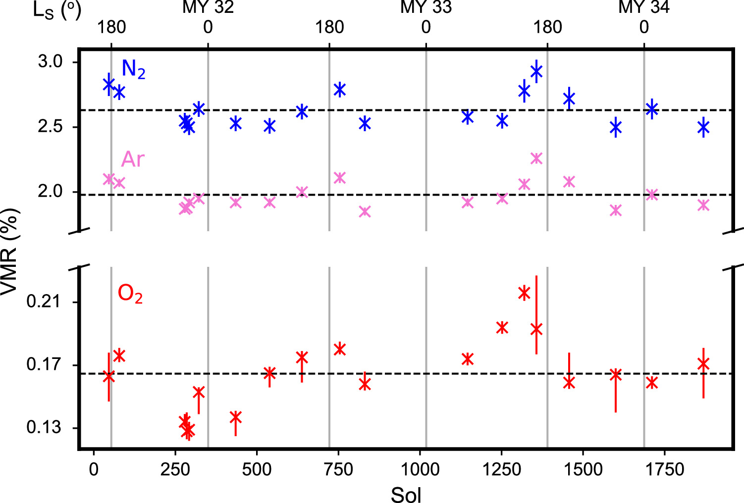
Figure A1. VMR measurements of N2 (blue), 40Ar (pink), and O2 (red) up to sol 1909 (Trainer et al. 2019). Dashed lines mark the means of the measurements for each species.
Download figure:
Standard image High-resolution imageTable A1. Volume Mixing Ratio Measurements of CO2, 40Ar, N2, and O2 up to Sol 1909 (Trainer et al. 2019)
| TID | Sol | LS | Ingest Start LMST | CO2 | 40Ar/10−3 | N2/10−3 | O2/10−3 | CO/10−3 |
|---|---|---|---|---|---|---|---|---|
| 25012 | 45.95 | 175.59 | 22:43 | 0.948 (0.001) | 21.0 (0.4) | 28.3 (0.9) | 1.63 (+0.15, −0.16) | 0.81 (0.05) |
| 25027 | 77.91 | 194.36 | 21:07, 22:42 | 0.949 (0.001) | 20.7 (0.3) | 27.7 (0.6) | 1.76 (+0.05, −0.04) | 0.72 (0.06) |
| 25084 | 278.58 | 320.79 | 13:02, 14:36 | 0.954 (0.001) | 18.7 (0.3) | 25.5 (0.6) | 1.34 (+0.05, −0.02) | 0.62 (0.03) |
| 25088 | 284.99 | 324.50 | 22:55, 00:30 | 0.954 (0.001) | 18.8 (0.3) | 25.3 (0.6) | 1.28 (+0.12, −0.05) | 0.56 (0.02) |
| 25095 | 292.13 | 328.58 | 02:25, 04:00 | 0.954 (0.001) | 19.2 (0.3) | 25.0 (0.6) | 1.29 (+0.05, −0.07) | 0.54 (0.09) |
| 25106 | 321.70 | 344.94 | 16:06, 17:41 | 0.952 (0.001) | 19.5 (0.3) | 26.4 (0.6) | 1.53 (+0.03, −0.14) | 0.57 (0.03) |
| 25150 | 434.91 | 40.91 | 21:07, 22:41 | 0.954 (0.001) | 19.2 (0.3) | 25.3 (0.6) | 1.37 (+0.04, −0.12) | 0.45 (0.03) |
| 25172 | 538.97 | 87.89 | 22:30, 00:05 | 0.954 (0.001) | 19.2 (0.3) | 25.1 (0.6) | 1.65 (+0.04, −0.09) | 0.42 (0.02) |
| 25195 | 638.08 | 134.69 | 01:05, 02:39 | 0.951 (0.001) | 20.0 (0.4) | 26.2 (0.6) | 1.75 (+0.04, −0.16) | 0.46 (0.12) |
| 25217 | 753.97 | 198.87 | 22:24, 23:58 | 0.949 (0.001) | 21.1 (0.4) | 27.9 (0.6) | 1.80 (+0.05, −0.03) | 0.64 (0.03) |
| 25232 | 830.91 | 247.85 | 21:05, 22:40 | 0.954 (0.001) | 18.5 (0.3) | 25.3 (0.6) | 1.58 (+0.08, −0.04) | 0.73 (0.03) |
| 25301 | 1145.99 | 60.23 | 22:57, 00:32 | 0.952 (0.001) | 19.2 (0.3) | 25.8 (0.6) | 1.74 (+0.04, −0.04) | 0.96 (0.15) |
| 25337 | 1252.02 | 108.30 | 23:37, 01:12 | 0.952 (0.001) | 19.5 (0.3) | 25.5 (0.6) | 1.94 (+0.04, −0.04) | 1.02 (0.10) |
| 25343 | 1319.68 | 141.28 | 16:18 | 0.948 (0.001) | 20.6 (0.4) | 27.8 (0.9) | 2.16 (+0.05, −0.05) | 1.08 (0.06) |
| 25346 | 1357.07 | 161.02 | 01:46 | 0.945 (0.001) | 22.6 (0.4) | 29.3 (0.9) | 1.93 (+0.34, −0.16) | 1.03 (0.06) |
| 25372 | 1457.07 | 220.39 | 01:35 | 0.949 (0.001) | 20.8 (0.4) | 27.2 (0.9) | 1.59 (+0.19, −0.04) | 1.10 (0.06) |
| 25395 | 1600.07 | 311.55 | 01:46 | 0.954 (0.001) | 18.6 (0.4) | 25.0 (0.8) | 1.64 (+0.04, −0.24) | 0.99 (0.06) |
| 25409 | 1711.06 | 11.86 | 01:26 | 0.951 (0.001) | 19.8 (0.4) | 26.4 (0.8) | 1.59 (+0.04, −0.04) | 1.20(0.07) |
| 25440 | 1869.07 | 84.70 | 01:42 | 0.953 (0.001) | 19.0 (0.4) | 25.0 (0.8) | 1.71 (+0.10, −0.22) | 0.99 (0.06) |
Note. Uncertainties, provided in parentheses, are symmetric except for O2.
Download table as: ASCIITypeset image
Appendix B: Photochemical Model Parameters
In this study we used a 1D globally averaged ion–neutral photochemical model to calculate the number density of various O-containing species and the rates of key reactions producing (P1)–(P7) and removing (L1)–(L3) O2 from the atmosphere. The reaction rate coefficients for calculating the rates of these key reactions are provided in Table B1.
Table B1. Reaction Rate Coefficients for (P1)–(P7) and (L1)–(L3)
| Reaction | k | Reference | |
|---|---|---|---|
| (P1) | 2O + M → O2 | 5.21 × 10⁻³⁵ e900/T [M] | Tsang & Hampson (1986) |
| (P2) | OH + O → O2 + H | 1.80 × 10⁻¹¹ e180/T | Burkholder et al. (2015) |
| (P3) | HO2 + O → O2 + OH | 3.00 × 10⁻¹¹ e200/T | Burkholder et al. (2015) |
| (P4) | HO2 + HO2 → H2O2 + O2 | 3.00 × 10⁻¹³ e460/T | Burkholder et al. (2015) |
| (P5) | NO2 + O → O2 + NO | 5.10 × 10⁻¹² e210/T | Burkholder et al. (2015) |
| (P6) | O3 + h ν → O2 + O | — | Heays et al. (2017) |
| (P7) | O3 + H → O2 + OH | 1.40 × 10⁻¹⁰ e−470/T | Burkholder et al. (2015) |
| (L1) | O2 + h ν → 2O | — | Heays et al. (2017) |
| (L2) | O2 + H → HO2 |
![$\tfrac{{k}_{0}[M]{k}_{\infty }}{{k}_{0}[M]+{k}_{\infty }}{0.6}^{\alpha }$](https://content.cld.iop.org/journals/2632-3338/5/3/65/revision1/psjad251bieqn6.gif) , k∞ = 2.40 × 10⁻¹¹
T0.2, k0 = 7.31 × 10⁻²⁹
T−1.3, , k∞ = 2.40 × 10⁻¹¹
T0.2, k0 = 7.31 × 10⁻²⁹
T−1.3, ![$\alpha =1+{\left({\mathrm{log}}_{10}\tfrac{{k}_{0}[M]}{{k}_{\infty }}\right)}^{2}$](https://content.cld.iop.org/journals/2632-3338/5/3/65/revision1/psjad251bieqn7.gif)
| Burkholder et al. (2015) |
| (L3) | O2 + O → O3 |
![$\tfrac{{k}_{0}[M]{k}_{\infty }}{{k}_{0}[M]+{k}_{\infty }}F$](https://content.cld.iop.org/journals/2632-3338/5/3/65/revision1/psjad251bieqn8.gif) ,k∞ = 2.80 × 10⁻¹², k0 = 5.29 × 10⁻²⁸
T−2.4, ,k∞ = 2.80 × 10⁻¹², k0 = 5.29 × 10⁻²⁸
T−2.4, ![$\mathrm{log}F=\mathrm{log}{F}_{c}{\left(1+{\left(\tfrac{\mathrm{log}({k}_{0}[M]{k}_{\infty }+C)}{(N-0.14(\mathrm{log}({k}_{0}[M]{k}_{\infty }+C)))}\right)}^{2}\right)}^{-1}$](https://content.cld.iop.org/journals/2632-3338/5/3/65/revision1/psjad251bieqn9.gif) , ,
| Atkinson et al. (1989); Burkholder et al. (2015) |
Download table as: ASCIITypeset image
Appendix C: Curiosity's Traverse over the Floor of Gale Crater
Over sols 45–1869 spanned by the atmospheric measurements used in this study, the Curiosity rover has traveled a total of 17.6 km on the floor of Gale crater as it studied the geology of Gale crater. Figure C1 provides a map of the traverse. The geology exposed on the surface can be broadly divided into the Bradbury and Mt. Sharp groups, with the transition occurring at the Pahrump Hill waypoint, which Curiosity arrived at on sol 753.
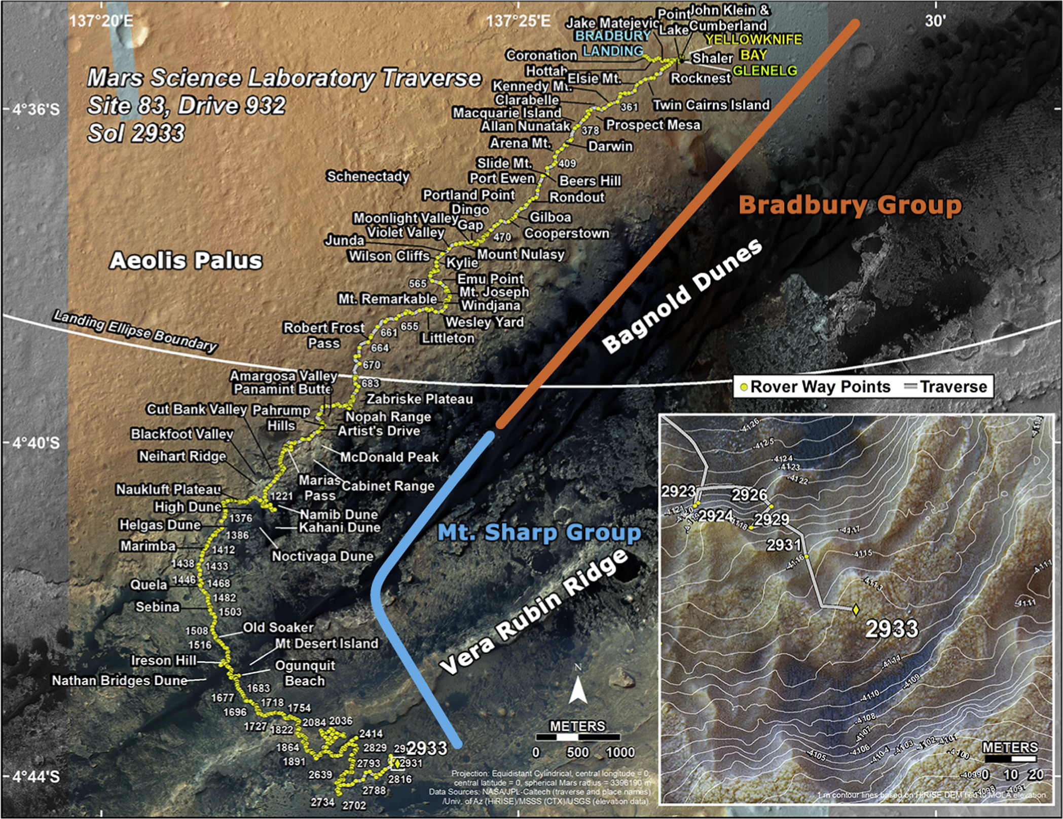
Figure C1. Curiosity's traverse map through sol 2933, with waypoint names and sol number of each drive. The division between the Bradbury and Mt. Sharp Groups, with the transition at Pahrump Hills, is shown. Image credit: NASA/JPL-Caltech/University of Arizona
Download figure:
Standard image High-resolution imageAppendix D: Variation of Normalized O2 with Various Variables
In this study, we investigated if variations in the normalized O2 VMR are associated with other atmospheric or geologic variables. Figure D1 presents correlation plots of the normalized O2 VMR with a variety of H2O-related variables. Figures D2, D3, and D4 show how, respectively, the WEH, thermal inertia and perchlorate concentration in the immediate vicinity of the Curiosity rover varies over the mission, with the normalized O2 VMR overplotted for comparison.

Figure D1. Correlation plots of the normalized O2 VMR with (a) maximum daily relative humidity as measured by MSL REMS, (b) minimum daily H2O VMR as measured by REMS, (c) rate of change of the REMS minimum daily H2O VMR in ppmv sol–1, and (d) WEH from MSL DAN. Horizontal error bars denote standard deviation over a ±30 sol window about the O2 measurements.
Download figure:
Standard image High-resolution image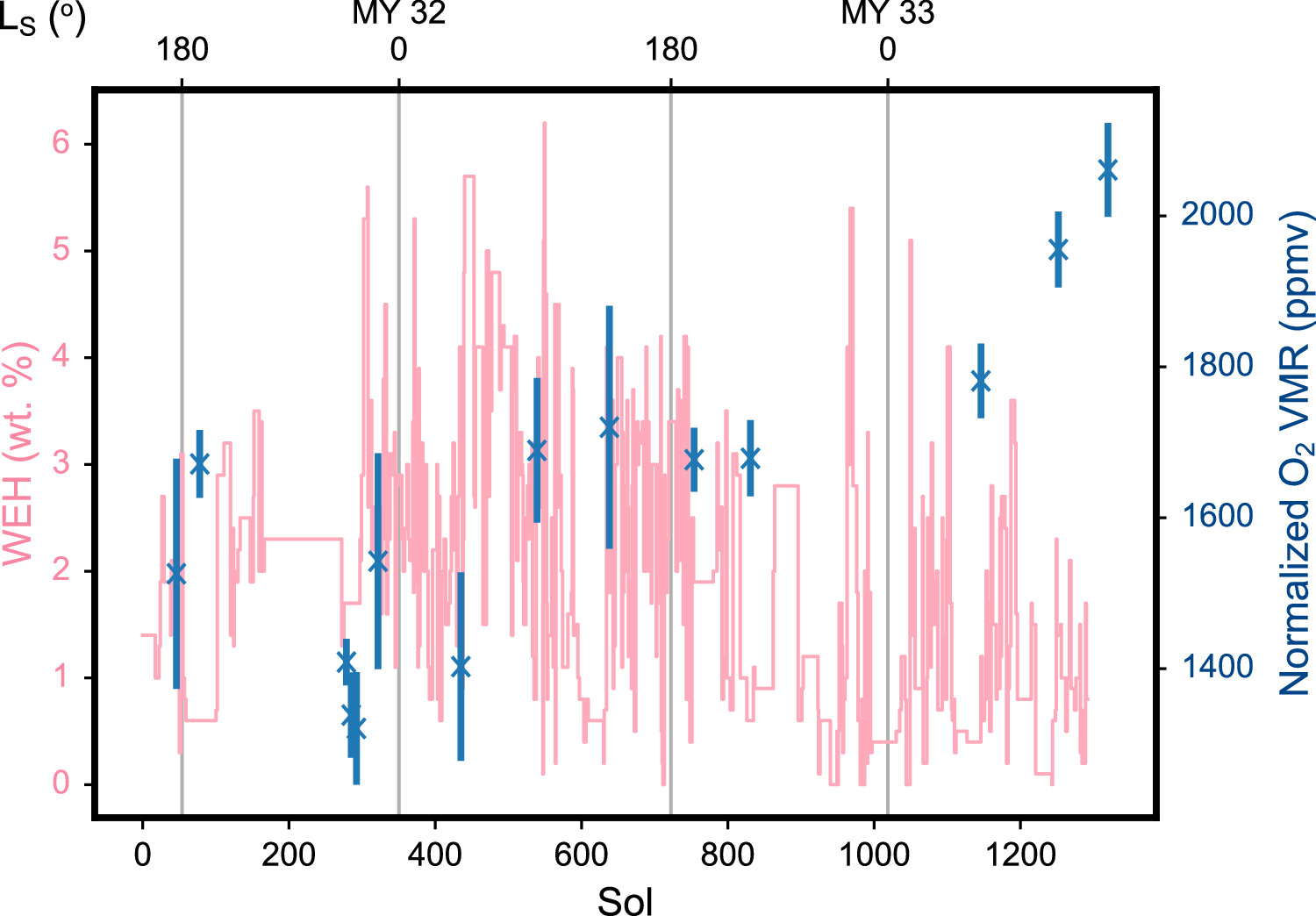
Figure D2. WEH (pink) as measured by DAN (Tate et al. 2018, 2019). Variations reflect changing geology from Curiosity's changing location, and horizontal lines mark periods when Curiosity remained stationary. Normalized O2 VMRs from Figure 1 (blue) are overplotted for reference.
Download figure:
Standard image High-resolution image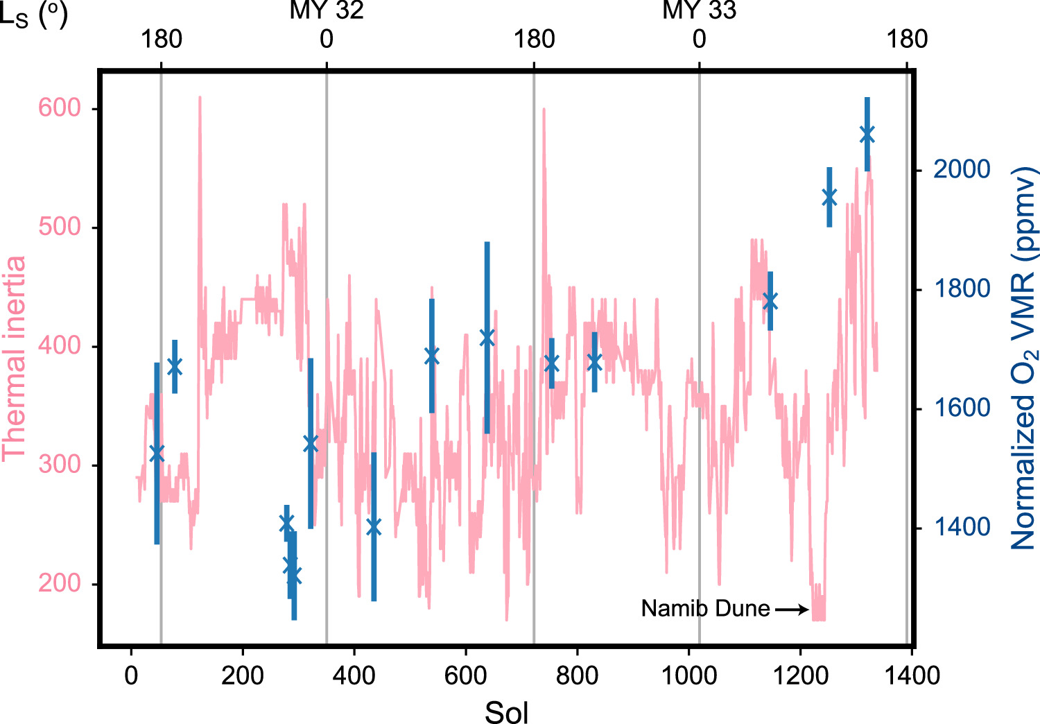
Figure D3. Thermal inertia (pink; in units of J m−2 K−1 s−0.5) over Curiosity's traverse from sol 30 to sol 1328 (Vasavada et al. 2017). Variations reflect the changing composition and nature (e.g., bedrock vs. unconsolidated fines) of the surface. Normalized O2 VMRs from Figure 1 (blue) are overplotted for reference.
Download figure:
Standard image High-resolution image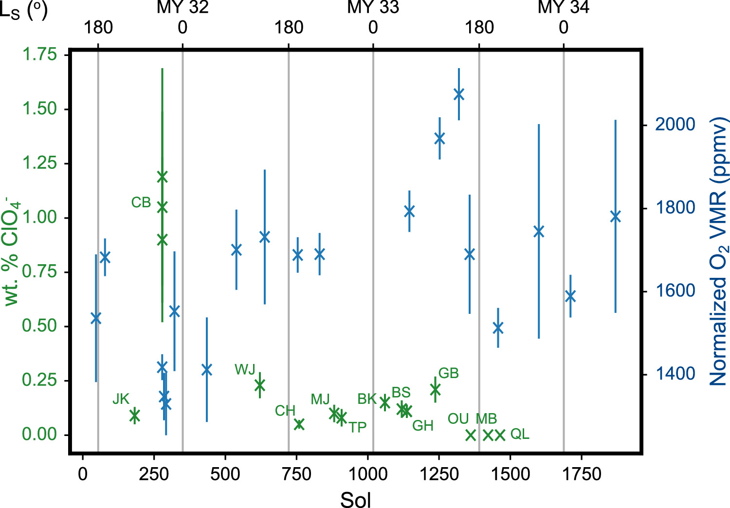
Figure D4. Perchlorate concentration in various solid samples (green) as determined from evolved O2 in SAM EGA experiments (Sutter et al. 2017; Clark et al. 2021), with the sol of sample acquisition. Labels provide the sample names (JK = John Klein; CB = Cumberland; WJ = Windjana; CH = Confidence Hills; MJ = Mojave; TP = Telegraph Peak; BK = Buckskin; BS = Big Sky; GH = Greenhorn; GB = Gobabeb; OU = Oudam; MB = Marimba; QL = Quela). No O2 peak was observed for the OU, MB, and QL samples (Clark et al. 2021). Normalized O2 VMRs from Figure 1 (blue) are overplotted for reference.
Download figure:
Standard image High-resolution imageAppendix E: Relevant Supporting SAM QMS Data
E.1. Background and Signal Trends for O2 and CO
In the original publication of the SAM mixing ratio data in Trainer et al. (2019), it was noted that after sol 1000 the retrieval of the CO VMR was suspect:
Although we have measured the CO in each atmospheric experiment through MSL sol 1,711, measurements after sol 1,000 show significantly elevated signal at m/z 12 and therefore very high CO mixing ratios. The VMR for CO obtained in MY 32, near LS 250° (MSL sol 830, TID 25232, Tables 1 and S1) shows the onset of this trend, in which the CO begins to diverge from the repeated seasonal trend in Ar (Figure 8). In addition to the derived CO mixing ratio, more than doubling from MY 32 to MY 33, the elevated measurements have not decreased or shown any seasonal modulation in MY 33 and MY 34, in contrast to the O2 measurement. This behavior is suspect, and at this time, a possible contamination or instrument effect cannot be ruled out. Especially because we know the m/z 12 signal to be highly sensitive to such effects (Franz et al. 2015), we are cautiously omitting the questionable observations from this paper. Those CO measurements thus require further investigation and will be reported at a later time.
It is important to note that the decrease in the confidence of the CO VMR derivation does not impact the O2 measurement that was reported, and that is the cornerstone of the work presented herein. One of the most important factors to consider is that the detection of CO is marginal, given its low relative abundance compared to CO2 and N2, both of which produce mass fragments that interfere with the CO signal in the mass spectrometer.
The primary peak for O2 is its molecular ion at m/z = 32, which is not impacted by the same factors as CO because (1) m/z = 32 is not a prevalent HC fragment (as compared to m/z = 12–14) and (2) it is the highest signal fragment for O2 and there is only a minor contribution from CO2.

Figure E1. Raw integrated peak areas for the mass channels used for the calculation of mixing ratios for O2 (m32) and CO (m12) for the QMS background and atmospheric ingests for multiple runs on Mars: TID 25012 = sol 45, TID 25232 = sol 830, TID 25343 = sol 1319, and TID 25440 = sol 1869. The figure is modeled after Figure 3 in Trainer et al. (2019) and includes the modeled background fits as described in that publication. Note that the calculation to remove the contribution of CO2 to m/z = 12 in order to derive CO mixing ratios happens after the background calculation is complete, and thus the corrected values are not shown with a background fit. They are provided in the plot to give a perspective to the magnitude and variation of signal in this mass channel during the progression of the mission.
Download figure:
Standard image High-resolution imageIt can be seen in Figure E1 that the background signal for O2 has been very stable throughout the mission, and there are no signs to indicate degradation of the instrument or changes in the performance at this mass channel. In contrast, the background for m/z = 12 shows more variability.
E.2. Ongoing SAM Atmospheric Measurements
Figure E2 shows the full set of atmospheric measurements that have been conducted by the SAM QMS to date that are available on PDS. The time of year/season of the measurements is indicated with the asterisk. Measurements have continued from MY 34, although not at the same cadence as the prior campaign that led to the Trainer et al. (2019) paper. Other mission measurement priorities, specifically the drilling and organic analysis measurements by the SAM instrument suite, have reduced the cadence of the atmospheric measurements. In particular, there was a large gap from mid–MY 34 to mid–MY 35 to allow the instrument resources to be dedicated to the solid sample analysis, a top priority for mission science. Currently, the mission is in the middle of a campaign to take measurements through the end of MY 37.

Figure E2. Atmospheric mixing ratio measurements completed by the SAM QMS on Mars since landing. All data are currently available at the PDS Geosciences node (https://pds-geosciences.wustl.edu/missions/msl/sam.htm).
Download figure:
Standard image High-resolution image
As noted in Trainer et al. (2019), high signal levels in the wet chemistry experiment on sol 1909 caused a shift in the sensitivity of the instrument detectors, requiring a change in the QMS electron multiplier gain setting. Mixing ratio determinations for atmospheric runs following that shift have indicated a change in the calibration ratios needed to properly derive the relative composition of the primary gases. In situ calibrations similar to that reported in Franz et al. (2017) have been performed on Mars, and the analysis of these data to derive new calibration constants is ongoing. At this time the team is not able to publish high-fidelity VMRs for this later data set that are of high enough confidence to support meaningful scientific interpretation.
Footnotes
- 5
1 Da = 1.6605390660(50) × 10−27 kg.
- 6
For clarity, we shall use "oxygen" to refer generally to an oxygen-containing species or reservoir, reserving "O2" and "O" for the specific molecular and atomic species.