

Abstract
Calculations are presented on the trajectory of a golf ball that rolls across the inclined surface of a golf green. The ball follows a curved path and comes to a stop at a point displaced at an angle to the initial launch direction. It is shown that the displaced angle is independent of the launch speed but depends on the launch angle and the ratio of the incline angle to the coefficient of rolling friction. The stopping distance is proportional to the launch speed squared. A simple experiment is described to check the calculations.
Export citation and abstract BibTeX RIS

Original content from this work may be used under the terms of the Creative Commons Attribution 4.0 licence. Any further distribution of this work must maintain attribution to the author(s) and the title of the work, journal citation and DOI.
1. Introduction
A major problem faced by all golfers is predicting the trajectory of the ball across a sloping green. The ball usually follows a curved path, although it will follow a straight line path if the ball is projected straight up or straight down the incline. The problem lies in estimating the launch speed and angle required for the ball to land either in the hole or to stop at a nearby spot. Limited assistance is available to golfers in the form of charts that show slope contours and green speeds, but golfers still need to use their own judgement of the required launch speed and angle, based on previous experience.
The physics of the problem involves acceleration of the ball down the slope due to the component of the gravitational force down the slope, plus the opposing friction forces due to static and rolling friction. Static friction ensures that the bottom of the ball comes to rest on the green if it rolls without slipping. Rolling friction allows the ball to roll to a stop up or down the slope if the slope is small enough [1]. The slope is typically less than three degrees near the hole. Specific trajectories of a ball rolling on a golf green have been calculated by Penner [2] and by Dewhurst [3], showing that the ball can curve towards or away from the hole depending on whether the ball is launched on a downhill or uphill slope respectively. The same approach is followed in the present paper to extract other results, not previously described, that apply more generally to the trajectories that are observed. In particular, it is shown that the ball comes to a stop after curving through an angle that is independent of the launch speed. Stopping distances are also calculated.
Numerical solutions are needed to determine the trajectories. The problem is similar to that when calculating trajectories of a ball through the air subject to lift and drag forces, apart from the fact the ball rolls on a golf green so the trajectory depends on rolling friction rather than aerodynamic forces. Regardless of whether the ball travels through the air or along the ground, the trajectory equations involve solutions of coupled nonlinear ordinary differential equations, so the results are more complicated than those involved in the motion of a ball projected vertically through the air or motion of a ball straight up or straight down an inclined surface.
There is an extensive literature on the physics of sport in physics teaching journals, illustrating physics encountered in undergraduate mechanics courses. The present article extends that literature to consider the trajectory of a ball rolling on an inclined surface. The basic physics is the same as that presented to undergraduate students. Newtonian physics comes to life when it is shown how it is relevant to practical problems of interest to students, such as those encountered in various sports.
2. Theoretical model
The geometry of the problem is shown in figures 1 and 2. The ball follows a curved path on an inclined plane tilted in the y direction at an angle θ to the horizontal. The coordinates of the ball on the inclined plane are x, y, the linear velocity of the center of mass of the ball is v, and the ball rolls without slipping if v = ω × R where × denotes the vector cross product, R is the ball radius (directed normal to the inclined plane) and ω is its angular velocity. The components of v and ω are related by vy = −R ωx and vx = R ωy as indicated in figure 1. Note that ωx is negative when vy > 0. For simplicity it is assumed that the ball is launched in a rolling mode. In practice, a putted ball usually slides for a short distance before it starts rolling [4], so the solutions given below are strictly only relevant after the ball starts rolling without slipping.

Figure 1. Geometry of a green sloping uphill at angle θ in the +y direction.
Download figure:
Standard image High-resolution imageAt any given time, v is inclined at an angle β to the y axis, as shown in figure 2(a). The gravitational force on the ball in the negative y direction is  , where m is the ball mass, and a friction force F acts at angle ϕ to the negative y direction. F represents the combined effect of rolling friction acting in a direction opposite the direction of v, plus a static friction force that acts in the positive y direction while the ball is rolling. The normal reaction force on the ball is
  and it acts at a distance D ahead of the center of mass, as it does whenever a ball is rolling [1, 2]. The x and y components of D are
  and
and  , as indicated in figure 2(a).

Figure 2. The normal reaction force, N, acts at a distance D ahead of the ball center.
Download figure:
Standard image High-resolution imageThe angular velocity components vary with time according to the relation R × F + D × N = Icmd ω /dt, with components

and

where Icm = (2/5)mR2 is the moment of inertia of the ball,  and
and  . Fx
points in the negative x direction and Fy
points in the negative y direction, while ωx
and ωy
are taken to be positive in a clockwise sense in figures 2(b) and (c).
. Fx
points in the negative x direction and Fy
points in the negative y direction, while ωx
and ωy
are taken to be positive in a clockwise sense in figures 2(b) and (c).
The acceleration of the ball in the x and y directions is given by

and

Given that vx = R ωy and vy = R ωx , then dvx /dt = Rdωy /dt and dvy /dt = Rdωx /dt, so Fx and Fy are given from equations (1) and (2) by

and

Substitution in equations (3) and (4) then gives the acceleration components

and

given that  . The direction of the friction force is given by

On a horizontal surface where θ = 0, the ball decelerates due to rolling friction, and μR = F/N is the coefficient of rolling friction. In that case N = mg, F = −μR mg so the ball decelerates with a = − μR g = −gD/1.4R from equations (7) or (8). Consequently,

Equation (9) can also be derived by assuming that the rolling friction force μR
mg acts in a direction opposite v and the static friction force  acts in the positive y direction, as it does when β = 0, F being the vector sum of the two friction forces. Equations (7) and (8) can be expressed in the form

and

where  ,
,  ,
,  and
and  . A and B can be taken as constants on any given incline, equal to the average values determined from Stimpmeter readings [2]. The various trajectories on the incline depend on the ratio B/A or on the ratio θ/μR
when θ is small. At any given launch speed and launch angle, the deceleration in the x direction is proportional to A and the deceleration in the y direction depends on B/A so the angular displacement from the initial launch direction depends on θ/μR
. If the launch speed, v0, is doubled on a given incline, and if the launch angle remains the same, then vx
/v and vy
/v remain the same so dvx
/dt and dy
/d
t remain the same but the ball takes twice as long to come to a stop and travels four times further. If A and B are increased by the same factor, then the deceleration will increase by the same factor in both the x and y directions, so the stopping distance will decrease by that factor. These effects are illustrated by numerical solutions in the following section.
. A and B can be taken as constants on any given incline, equal to the average values determined from Stimpmeter readings [2]. The various trajectories on the incline depend on the ratio B/A or on the ratio θ/μR
when θ is small. At any given launch speed and launch angle, the deceleration in the x direction is proportional to A and the deceleration in the y direction depends on B/A so the angular displacement from the initial launch direction depends on θ/μR
. If the launch speed, v0, is doubled on a given incline, and if the launch angle remains the same, then vx
/v and vy
/v remain the same so dvx
/dt and dy
/d
t remain the same but the ball takes twice as long to come to a stop and travels four times further. If A and B are increased by the same factor, then the deceleration will increase by the same factor in both the x and y directions, so the stopping distance will decrease by that factor. These effects are illustrated by numerical solutions in the following section.
Equations (11) and (12) can also be cast in the simpler form

and

where Vx
= vx
/v0, Vy
= vy
/v0, V = v/v0, 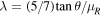 and
and  . In that case, the only relevant parameters of the model are β(0) and λ, while v0 is a scaling factor. The dynamic behaviour is therefore not affected by v0, apart from the fact that the stopping distance and time does depend on v0.
3. Numerical solutions
Numerical solutions of equations (11) and (12) to calculate vx and vy , and then the coordinates x and y, were obtained by a predictor-corrector method, but other methods are likely to work just as well. Solutions are shown in figure 3 for a ball launched uphill at an angle β(0) = 80° to the y axis with initial speed v0 = 1.5 or 2.0 m s−1. In figure 3(a), θ = 1° and μR = 0.05. In figure 3(b), θ = 2° and μR = 0.1. The ball is launched up the incline but it curves back down the incline before coming to a stop.
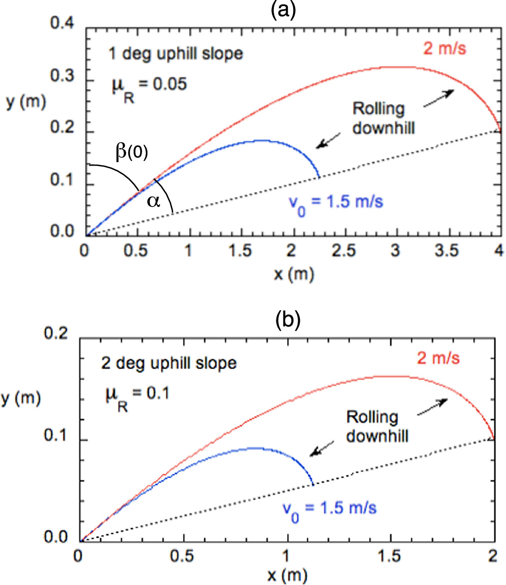
Figure 3. Trajectories on an uphill slope when the ball is launched at β(0) = 80° with (a) θ = 1° and μR = 0.05 or (b) θ = 2° and μR = 0.1.
Download figure:
Standard image High-resolution imageIn figure 3(a) and also in figure 3(b), the x, y coordinates of the higher speed launch are a factor of  larger than the coordinates of the lower speed launch, meaning that both trajectories are identical if the x and y coordinates of the low speed trajectory are multiplied by a factor of 1.778. Consequently, the ball comes to a stop after curving through the same angle, α, away from the launch angle, as shown in figure 3(a). Figure 3(b) differs from figure 3(a) in that θ and μR
are both twice as large in figure 3(b), with the result that the x, y coordinates are smaller by a factor of two. The angle α is the same for all four trajectories, but the stopping distance of the ball is reduced by a factor of two in figure 3(b). Other numerical results show that at any given launch speed v0 and launch angle β(0), if θ and μR
are both increased by the same factor F then the stopping distance decreases by a factor F but the angle α is unaffected.
larger than the coordinates of the lower speed launch, meaning that both trajectories are identical if the x and y coordinates of the low speed trajectory are multiplied by a factor of 1.778. Consequently, the ball comes to a stop after curving through the same angle, α, away from the launch angle, as shown in figure 3(a). Figure 3(b) differs from figure 3(a) in that θ and μR
are both twice as large in figure 3(b), with the result that the x, y coordinates are smaller by a factor of two. The angle α is the same for all four trajectories, but the stopping distance of the ball is reduced by a factor of two in figure 3(b). Other numerical results show that at any given launch speed v0 and launch angle β(0), if θ and μR
are both increased by the same factor F then the stopping distance decreases by a factor F but the angle α is unaffected.
Downhill trajectories are not the same as uphill trajectories but the same general features are found, apart from the fact that the ball curves in the opposite direction. The y displacement of the ball is also much larger in the downhill direction, as indicated in figure 4 where the ball is launched down a 1° incline with the same initial parameters as in figure 3(a).

Figure 4. Trajectories on a one degree downhill slope when the ball is launched at β(0) = 80°.
Download figure:
Standard image High-resolution imageThe break angle, α, depends on the launch angle as well as the θ/μR ratio but is independent of the launch speed at any given launch angle. Typical results are shown in figure 5 for uphill and downhill putts at three different launch angles. In practice, θ can vary from zero to about 3◦ and μR varies from about 0.04 for a fast green to about 0.09 for a slow green, so θ/μR can vary from zero up to about 75. The break angle is only slightly larger for downhill putts, despite the fact that the stopping distance is generally much larger. For example, α = 7.2° in figure 3 and α = 7.5° in figure 4, both with θ/μR = 20 and β(0) = 80°.
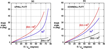
Figure 5. Break angle, α, for (a) uphill and (b) downhill putts versus θ/μR .
Download figure:
Standard image High-resolution image4. Stopping distance
The stopping distance, S, is easily calculated on a horizontal surface and is equal to  . The stopping distance is also proportional to
  on an inclined green but the variation with θ and μR
is not simply expressed in analytical terms, apart from cases where the ball is launched straight uphill or straight downhill. In the latter cases,
on an inclined green but the variation with θ and μR
is not simply expressed in analytical terms, apart from cases where the ball is launched straight uphill or straight downhill. In the latter cases, 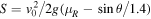 , assuming that θ is negative for a downhill putt.
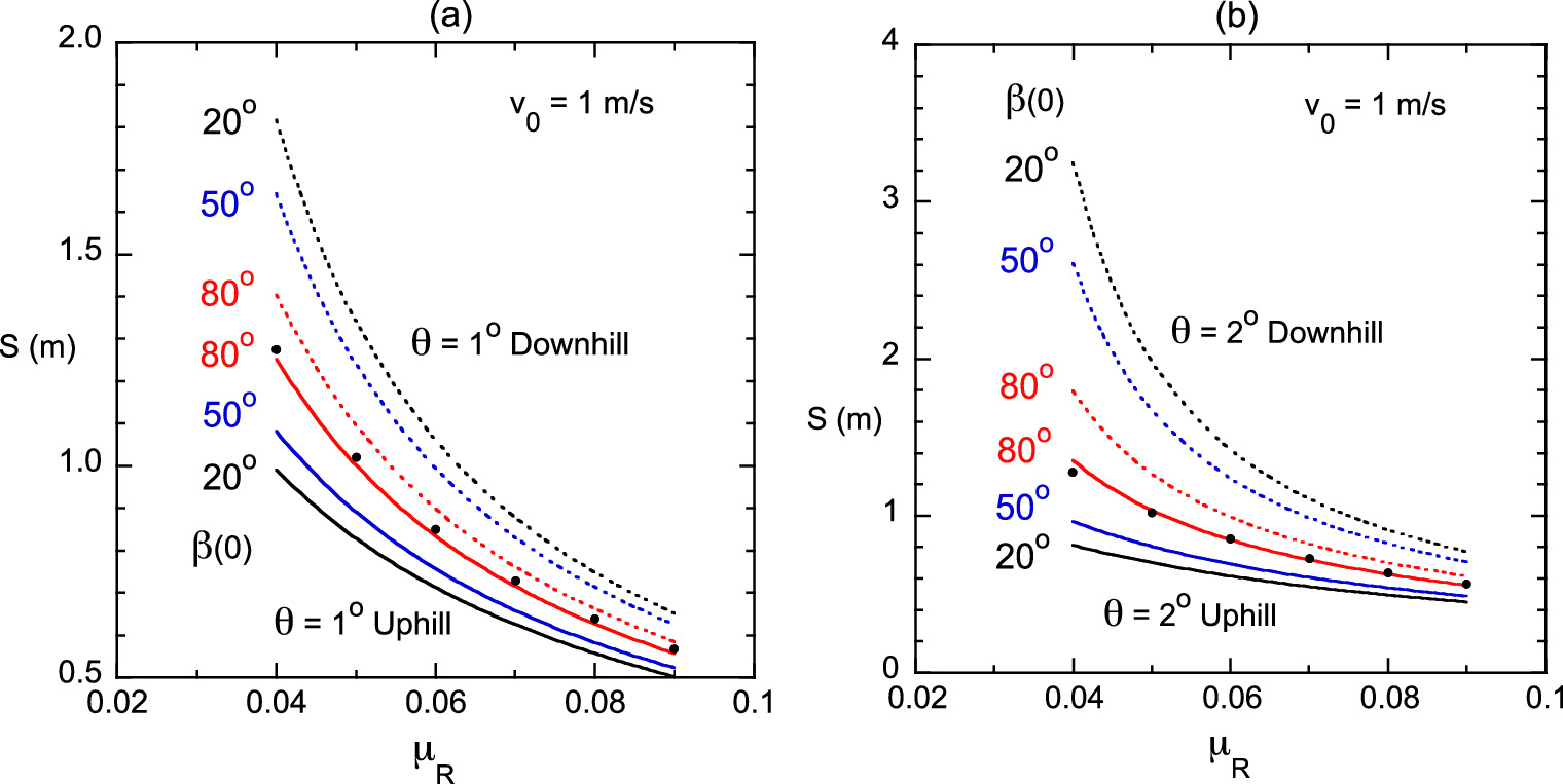
Numerical solutions with v0 = 1.0 m s−1 are shown in figure 6 for uphill and downhill putts on θ = 1° and 2° slopes. The stopping distance, S, is taken as the straight line distance from the launch point to the stopping point, but the actual distance travelled by the ball along its curved path is longer. All of the curves in figure 6 can be fit by power laws of the form  but n is different for every curve and varies from 0.73 to 1.75 while k varies from 0.01 to 0.08. The parameters n and k vary smoothly with β(0) but the relations are nonlinear. There is therefore no simple rule of thumb that a golfer can use to predict the stopping distance when θ or β(0) is varied, apart from the fact that the stopping distance increases as v0 increases, or when μR
decreases, or as β(0) decreases when putting downhill or as β(0) increases and when putting uphill. One useful hint is that the stopping distance when putting at β(0) = 80° uphill is almost the same as putting on a horizontal surface. Golfers will know these trends from experience anyway, and green books are readily available showing laser scanned slope contours for all major golf courses, but even professional golfers still have problems estimating or executing the appropriate launch speed [5].
but n is different for every curve and varies from 0.73 to 1.75 while k varies from 0.01 to 0.08. The parameters n and k vary smoothly with β(0) but the relations are nonlinear. There is therefore no simple rule of thumb that a golfer can use to predict the stopping distance when θ or β(0) is varied, apart from the fact that the stopping distance increases as v0 increases, or when μR
decreases, or as β(0) decreases when putting downhill or as β(0) increases and when putting uphill. One useful hint is that the stopping distance when putting at β(0) = 80° uphill is almost the same as putting on a horizontal surface. Golfers will know these trends from experience anyway, and green books are readily available showing laser scanned slope contours for all major golf courses, but even professional golfers still have problems estimating or executing the appropriate launch speed [5].

Figure 6. Stopping distance, S, for uphill and downhill putts versus μR when v0 = 1 m s−1 and (a) θ = 1° and (b) θ = 2°. Uphill putts are shown by solid curves. Downhill putts are shown by dashed curves. Dot points show the variation of S with μR on a horizontal surface.
Download figure:
Standard image High-resolution imageA visual summary of results is shown in figure 7 for stopping distances of 3 m on a green with θ = 2° and μR = 0.05. Trajectories are shown starting at 12 different launch points, together with the launch speeds required for the ball to stop in the middle of the hole. Left to right and right to left trajectories are symmetrical, but uphill and downhill trajectories are not. Similar information is provided by Aimpoint Golf (https://aimpointgolf.com) in the form of commercially available charts indicating the expected break angles or distances on greens with a variety of different slopes and different green speeds.

Figure 7. Trajectories and launch speeds for uphill and downhill putts on a green with θ = 2° and μR = 0.05, when S = 3.0 m. Dotted lines are straight lines from the launch point to the hole.
Download figure:
Standard image High-resolution image5. Experimental result
In order to check the calculations, an experiment was conducted using a small incline covered in a towel to simulate a putting green. A golf ball was projected up and across the incline and its trajectory was determined by filming from above at 300 frames s−1, using Tracker software to digitise the ball coordinates. The arrangement is shown in figure 8. The ball was launched by hand so that it would commence rolling without sliding. A typical result is shown in figure 9, together with a theoretical fit. The ball speed decreased almost to zero at the top of its trajectory and then accelerated down the incline since the incline angle was larger than that of a typical golf green. The main point of interest was to determine whether equations (11) and (12) provide a good description of a rolling ball on an incline.

Figure 8. Experimental arrangement.
Download figure:
Standard image High-resolution image
Figure 9. Experimental ball trajectory (shown as dots) on a θ = 5.9° incline. The smooth curve is a numerical solution of equations (11) and (12).
Download figure:
Standard image High-resolution image
Values for μR and the slope of the incline were determined from the accelerations aU and aD straight up and straight down the incline respectively. From equation (12), with β = 0 up the incline and β = 180° down the incline,

and

The measured value of μR depended on the ball speed, being as large as 0.07 at speeds less than 0.1 m s−1 and as small as 0.03 at speeds above 0.2 m s−1. A good theoretical fit to the measured trajectory was obtained with μR = 0.06 when v < 0.2 m s−1 and μR = 0.03 when v > 0.2 m s−1. There is a small discrepancy between the theoretical and experimental trajectories as the ball starts descending down the incline, presumably due to the variation in μR with rolling speed. Similar results were obtained at other launch angles and launch speeds. Other possible golf ball trajectories could be investigated by students using an arrangement similar to that shown in figure 8 or to investigate the behaviour of other balls on other surfaces. A result using a billiard ball on a smooth incline is described in reference [6].
6. Conclusion
The motion of a golf ball rolling on a sloping green can be calculated analytically if the ball decelerates straight up or down the incline. More generally, the ball follows a curved path if it is projected at other angles. Numerical solutions are presented showing that the ball curves through an angle that is independent of the initial ball speed and that depends only on the launch angle and the θ/μR ratio or the equivalent parameter λ. The displacement angle is slightly different for uphill and downhill launches. The stopping distance is proportional to the square of the launch speed and increases as μR decreases, as it does on a horizontal surface, but there appears to be no other simple relation that determines how the stopping distance depends on the launch angle or the slope or speed of the green.
Data availability statement
All data that support the findings of this study are included within the article (and any supplementary files).
Author declaration
Conflict of Interest
The author has no conflicts to disclose.