

Abstract
This paper proves the theorem of uniqueness for the solution of a coefficient inverse problem for the wave equation in (with two unknown coefficients: speed of sound and absorption. The original nonlinear coefficient inverse problem is reduced to an equivalent system of two uniquely solvable linear integral equations of the first kind with respect to the sound speed and absorption coefficients. Estimates are made, substantiating the multistage method for two unknown coefficients. These estimates show that given sufficiently low frequencies and small inhomogeneities, the residual functional for the nonlinear inverse problem approaches a convex one. This solution method for nonlinear coefficient inverse problems is not linked to the limit approach as frequency tends to zero, but assumes solving the inverse problem using sufficiently low, but not zero, frequencies at the first stage. For small inhomogeneities that are typical, for instance, for medical tasks, carrying out real experiments at such frequencies does not present major difficulties. The capabilities of the method are demonstrated on a model inverse problem with unknown sound speed and absorption coefficients. The method effectively solves the nonlinear problem with parameter values typical for tomographic diagnostics of soft tissues in medicine. A resolution of approximately 2 mm was achieved using an average sounding pulse wavelength of 5 mm.
Export citation and abstract BibTeX RIS
1. Introduction
This article is concerned with developing effective methods for solving multi-coefficient inverse problems of wave tomography. Recently, there has been increased interest in tomographic imaging methods using ultrasonic, electromagnetic, and seismic radiation sources [1–5]. One interesting application of ultrasonic tomographic methods is early-stage breast cancer diagnosis [6–10]. Such applications require tomographic devices featuring high resolution and high accuracy. The most suitable mathematical model is the scalar wave model based on the hyperbolic differential equation, taking into account diffraction effects as well as absorption of ultrasonic waves. The inverse problem in this case is to reconstruct two unknown coefficients of the differential equation as functions of the coordinates.
Ultrasonic diagnostic methods are also widely used in nondestructive testing (NDT) [11–13]. A large number of studies on ultrasonic diagnostics in NDT and in medicine are focused on using reflected radiation. Ultrasonic tomographic methods being developed use the waves transmitted through the object in addition to reflected waves. Transmitted radiation provides the ability to perform quantitative characterization of inhomogeneities in the inspected objects with high accuracy. Such possibilities in real NDT experiments are presented in [14–16] assuming the scalar wave model. Some publications are concerned with solving inverse problems of tomographic ultrasonic diagnostics in a vector model, which supports transverse, surface, and other types of waves propagating in the medium in addition to the longitudinal wave [17–19].
This work is dedicated to the development of effective methods for solving two coefficient inverse problems in wave tomography under a model that takes into account both diffraction and absorption effects. From a mathematical point of view, the inverse problem is to minimize the residual functional between the wave field on the detectors, measured in the experiment, and the wave field computed using the given equation coefficients. The works [4, 20–26] provide representations for the gradient of the residual functional with mathematical rigor, which justifies minimizing the functional using iterative methods. Iterative methods of solving coefficient inverse problems for the wave equation based on minimizing the residual functional in application to seismic imaging are often referred to as the full waveform inversion (FWI) methods by the geophysical community [4]. The peculiarity of seismic imaging tasks is that typically seismic sources and receivers can be located only on the surface of the Earth. FWI approaches are also applicable to ultrasound imaging in NDT [11, 12].
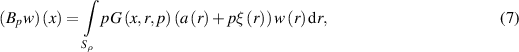
The problem with wave tomography is that the functional is not convex and may have local minima. A large number of studies [16, 27–31] are dedicated to finding global minima of functionals. This phenomenon is referred to as cycle skipping in the FWI community. This problem is well known and various approaches have been developed to solve it. Data-domain methods are based on the modification of the misfit measurement [28]. Another approach uses multiple steps to solve the inverse problem. At the first stage, low-pass filtered signals are used, in subsequent stages the frequency is gradually increased. In various modifications, this approach is presented as the method of choice [30], multi-scale FWI in time or frequency domain [4, 32]. This paper uses this approach in the multistage method (MSM) as a gradient iterative method for solving wave tomography problems in the time domain. This paper provides estimates showing that at sufficiently low frequencies the nonlinear inverse problem approaches а linear problem and the residual functional approaches а convex one. This characteristic of inverse problems in wave tomography underlies the MSM method.
Another important problem in wave tomographic diagnostics is the uniqueness of the solution to inverse problems. The problem of uniqueness of solutions to coefficient inverse problems is explored in the works [33–38]. In this paper, a theorem is proven on the uniqueness of the solution to the inverse problem of ultrasonic tomography in  under a model that takes into account both diffraction effects and absorption. A reduction of the nonlinear inverse problem to a system of linear integral equations is proven for the limit approach as sounding frequency tends to zero.
Supercomputers are used to develop gradient iterative methods in this study. The effectiveness of the algorithms is illustrated by model calculations, which represent a case of tomographic diagnostics of soft tissues.
2. Formulation of the inverse problem
In this study, we consider waves described by the scalar wave equation with absorption taken into account. The scalar model facilitates computing the scalar wave field  from given initial data using the equation


Here  is the wave speed in the medium;
  describes absorption in the medium;
  ;
;  is the Laplace operator on the variable
  ;
;  is the Dirac function, which specifies the position of the point source at
  . The sounding pulse generated by the source is described by the function.
The inverse problem of ultrasound tomography can be formulated as follows. Assume that the inhomogeneity of the medium is localized within the region  . Let us suppose that the positions of the wave sources, characterized by the parameter
  , together form a set
  , and
, and  does not intersect with
  The measurements of the field
  are available at points
  , which collectively form a set
  , which does not intersect with
  (figure 1).
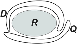
Figure 1. The scheme of the experiment in the formulation of the problem.
Download figure:
Standard image High-resolution imageWe assume that  ,
,  are smooth functions in
  ,
,  differs from the known constant
  only within the inhomogeneity of the medium (
 ),
),  differs from 0 also only within the inhomogeneity of the medium (
 ). For simplicity, we will set the function
  that describes the sounding pulse to
  . In the inverse problem, the objective is to determine the unknown functions
  and
and  for
for  , using the experimental data
  obtained at points
  (
( ) for various positions of the source
  . The inverse problem of wave tomography in the given setting is a nonlinear coefficient inverse problem. The inverse problem of determining the coefficients of the wave equation was studied in works [39, 40].
3. Uniqueness of the solution to the inverse problem. Reduction of a nonlinear coefficient inverse problem to a system of two linear integral equations of the first kind
We investigate the problem of uniqueness of the solution to the considered inverse problem in  . To do this, we reduce the nonlinear inverse problem to an equivalent system of two uniquely solvable linear integral equations for the coefficients
  and
and  . This approach largely repeats the methods used in [33] for the wave equation containing not two, but only one unknown coefficient
  . The problem of the uniqueness of the solution to the inverse problem of determining two coefficients
  and
and  in
in  was considered in [34], where the Laplace transform and the limit approach as
  for the Green's function of the operator
  were applied to equation (1) with
  as the Laplace transform parameter. This technique is not suitable in the case of
  space, since the Green's function for a two-dimensional space has a logarithmic singularity. The problem of the uniqueness of the solution to the inverse problem of determining a single coefficient
  in
in  and the reduction of the nonlinear coefficient inverse problem to a linear integral equation of the first kind was considered in [35–38]. Let us present more rigorous mathematical formulations of the inverse problem.
Condition 1. Let  and
and  be twice continuously differentiable functions on
  . We also assume that the function
  and its partial derivatives with respect to up to the second order have the Laplace transform defined for all
  , where
  ,
,  .
.
The Laplace transform is considered in the sense of generalized functions. As is known, this condition for the presence of the Laplace transform for the problem under consideration is not too limiting [33].
Condition 2. Let  be a bounded domain with a piecewise smooth boundary. D and Q are closed piecewise smooth curves that do not enclose the domain
  and do not intersect the closure
  .
.
We introduce the function  , where
  is the wave velocity in a homogeneous medium surrounding the investigated inhomogeneity. Then, after the Laplace transform on equation (1), we obtain

where  denotes the Laplace transform
  ,
,  . It is known that the Green's function for the operator on the left side of (3) has the following form in
  :
:
where  is the Macdonald function. Then equation (3) can be written as

Dividing both sides of the equation (4) by  , where

 , we obtain the equation
where  and
and  is a circle of radius
  , such that
  .
.
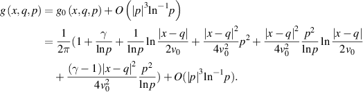
In [33], the following representation was obtained for  :
:
where  is the Euler–Mascheroni constant.
Consider the operator 
where  ,
,  .
.
Following the work [33], some properties of the operator  can be clarified. Since
  is continuous on
  , and the kernel of the operator
  has the form (6), according to the properties of the potential-type operator from [41], it follows that the operator
  is completely continuous for all
  From (6), it follows that
  , so for a sufficiently small
  , for all
  the norm
  . Then for all
  , denoting
  , from (5) it follows

Due to the continuity of  by
by  , for simplicity we consider only real
  . Then from (6) and (8), as well as using the representation
We can represent
Assuming that  , we can divide both sides by
  . As a result, similarly to [33], we have a power series expansion in terms of the small parameter
where the terms with  are included in
  Evaluating the limits for
  , we obtain a linear Fredholm integral equation of the first kind, which is called Lavrentiev's equation [35], for determining
  :
:

where


moreover,  can be computed from the data without knowing
  and the limits exist. From equation (11) we find
  . Furthermore, the following equations are satisfied:
Next,  can be determined if
  is known. Dividing equation (10) by
  and transferring the terms with
  to the left side, we obtain:
Similarly to (10), we have a power series expansion for  in terms of the small parameter
  , where
 ![$q \in Q,\,\,x \in D,\,\,p \in \left( {0,\varepsilon } \right],\,\varepsilon \in \left( {0,{e^{ - \gamma }}} \right]$](https://content.cld.iop.org/journals/0266-5611/40/4/045026/revision2/ipad2aa9ieqn110.gif) . Evaluating the limit for
. Evaluating the limit for  , we obtain a linear Lavrentiev integral equation for determining
  :
:

где
where  depends on the previously obtained
  but can be computed from the data without knowing
  and the limits exist. Furthermore, the following equations are satisfied:
A significant number of works are concerned with proving the uniqueness of the solution of Lavrentiev's equation under various conditions imposed on the sets  in
in  and
and  [33, 37, 42]. These works provide proof of the theorem that equations of the type (11), (14) on
  in the given statement have no more than one solution in the class C(R) of continuous functions in region R. Using this result, we formulate the following theorem.
- (a)Assume that conditions 1 and 2 for
 , , and for sets , R from the problem statement are met. Then the inverse problem of finding the functions , for equation (1) has a unique solution in the class C(R).
 - (b)


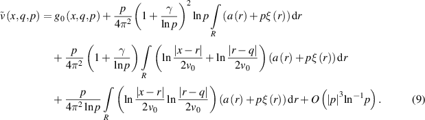
4. MSM and its substantiation
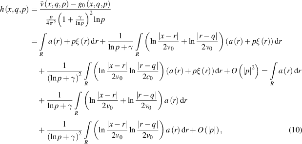
Theorem 1, besides proving the uniqueness of the solution to the inverse problem, also substantiates the reduction of the original nonlinear coefficient inverse problem to a system of two linear integral equations of the first kind with respect to functions  and
and  . The numerical solution of linear integral equations is not a problem. However, the possibility of reducing the original nonlinear problem to a linear one depends on the presence of very low (close to 0) frequencies in the spectrum of the sounding signal. This is difficult to achieve in physical experiments. In addition, solving the obtained first-kind integral equations is a highly unstable problem due to the form of the kernel of the integral operator, among other things. The numerical solution of the inverse problem with integral operators of this type has a low spatial resolution that is unacceptable in tomographic imaging [43].
Iterative methods for minimizing the residual functional  between the experimental data on the contour D and the wave field computed from equations (1) and (2) for given
  and
and  have proven effective for solving inverse problems with respect to parameters
  and
and  [44, 45].

Here  are the experimental data on the contour
  over time (0,T), and
  is the wave field obtained via solving the direct problems (1) and (2), which depends on the given coefficients
  and
and  . For multiple positions of the sounding radiation sources, the residual functional is a sum for
  of the residual values obtained for each source position. For each fixed source
  , the integral is summed over time (0,T) and over the contour
  containing all the detectors receiving the signals from the selected source. Mathematically, the inverse problem is posed as the problem of finding functions
  and
and  that minimize the residual functional (16):
  . The functions
  and
and  are taken as an approximate solution to the inverse problem.
The residual functional  can be efficiently minimized using gradient methods. The gradient of the functional
  defined by expression (16) has the form [44, 45]:

where  is the solution to the main problems (1) and (2), and
  is the solution to the conjugate problems (18) and (19). Both solutions depend on coefficients
  and
and  .
.


A typical situation for nonlinear problems is a non-convex residual functional  that may have local minima. As a result, using gradient methods of functional minimization with arbitrary initial approximation guarantees the convergence only to a local minimum, but not to the global minimum.
Let us consider another approach to solving the problem of nonlinearity, not related to the reduction of the original nonlinear inverse problem to a system of linear integral equations of the first kind (11), (12) and (14), (15). Unlike the reduction to a linear problem, we will not evaluate the limits for  , but instead we will use sufficiently low (but not equal to 0) frequencies at the first stage. This constitutes the so-called MSM.
Let slightly stronger conditions than condition 1 be satisfied. We assume that the function  and its partial derivatives with respect to
  up to the second order have a Laplace transform defined for all
  , where
  ,
,  . That is, it is additionally assumed that there is a Laplace transform for imaginary
 . The Laplace transform here is defined over generalized functions. Applicability of this condition was studied in detail in [33]. It was noted that this condition is not too restrictive. In particular, it holds for the Green's function
  of the wave equation in homogeneous space
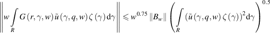
Using the approach described above in deriving equation (3), the Helmholtz equation with absorption can be represented as follows:

where  is the sounding frequency,
  . Using the Green's function method for the operator on the left side of equation (20), we can write:
where  is the Hankel function of the second kind,
  . As is known,
  and
and  , where
  is the Macdonald function from (6). Consequently, the estimates obtained earlier for the Macdonald function are valid for the Hankel functions.
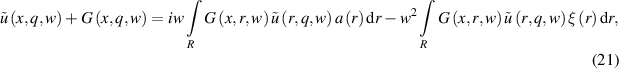
Equation (21) is a nonlinear integral equation with respect to  and
and  . Denoting
  , the equation (21) can be represented in another form, which highlights the first term of the Born series.
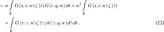
The first term on the right-hand side of (22) is the Born approximation of the scattering problem and takes the form of a linear integral operator with respect to  . The second term on the right-hand side of (22) has a multiplier
  and two multipliers
  under the integral. For sufficiently small values of
  and for
  , the second term on the right-hand side of equation (22) becomes a small quantity compared to the first term, and equation (22) becomes close to a linear equation. Therefore, the functional (16) becomes close to a convex one.
Let us formulate this more rigorously by writing equation (22) as follows:
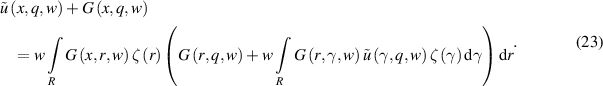
Let us show that the following limit is zero:
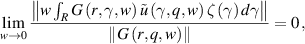
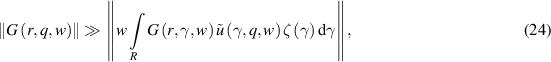
that is, for sufficiently small w, the inequality which we will call the condition of closeness to the linear problem holds:
where ||⋅|| is the norm in  . For the Green function
  , from (6) it follows that for all sufficiently small
 for some
  . Due to the boundedness and continuity of functions
  and
and  , the inequality
  holds for some
  . From the energy inequality for the Helmholtz equation,
  for some
  . Consider the operator
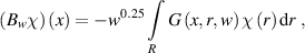
where  ,
,  . According to the properties of a potential-type operator from [41], the operator
  is completely continuous. From (6), it follows that
  , so that
  for all sufficiently small
  . Thus, for sufficiently small
  the following inequality holds:
The idea that for small heterogeneities  and sufficiently small
  the nonlinear inverse problem approaches a linear problem and the residual functional becomes convex is at the core of the MSM. The MSM algorithm consists of the following steps. The initial approximation is chosen as constants
  for the speed of sound and
  for the absorption factor, where
  is a known speed of sound in the homogeneous medium surrounding the imaged object. Experimental data at two (or more) different central frequencies
  and
and  are used,
  . First, the inverse problem is solved using iterative methods using the data for the lower frequency
  , and a constant initial approximation. At low frequencies, the residual functional approaches convex and the iterative minimization process does not encounter local minima. Then, at the second stage, the inverse problem is solved using the higher frequency
  to improve the resolution. The speed of sound and absorption factor obtained via solving the inverse problem at the first stage using the lower frequency
  are used as the initial approximation for the second stage. The process continues further if more than two central frequencies are chosen.
Note that in this article, experimental data with a central frequency  is understood as data obtained by sounding with a broadband pulse with a central frequency
  and the problem is solved in the time domain. It is also possible to perform sounding with harmonic signals with different frequencies and solve the problem in the frequency domain for the Helmholtz equation.
In the provided estimates of the approximation of the nonlinear inverse problem with a linear one at sufficiently low frequencies, nothing is said about the specific values of the parameters of scattering objects and the frequencies in a specific problem. Let us try to estimate the scattering wave function depending on the parameters of the scattering object and the frequency, in order to determine at what values of  and
and  inequality (24) holds.
The integral in inequality (24) represents the scattered wave  in the area of heterogeneity
  . The expression for the scattered wave can be obtained by following the results of [46] for perturbation theory in quantum mechanics in the WKB approximation. Let us consider the equation for the scattering wave function
  for a small scatterer
  ,
,  , which is similar to equation (20) without taking into account the point source of radiation

where  . Let the incident plane wave propagate along the х-axis. In the first approximation, the wave function depends on the coordinates in the same way as the incident plane wave propagating along the x-axis. Therefore, we seek a solution in the form
  , where
  changes slowly compared to
  . Substituting
  into equation (26), we obtain:

We simplify this expression by dividing by  For large
  and slowly varying
  we can neglect the second derivatives of
  , then
So,
In physical media heterogeneous in speed and absorption, according to formula (21), the scattering function has the form  . Substituting
  into (27), we get

where  is the size of the heterogeneity
  from the beginning of the heterogeneity to point
  along the line parallel to the x-axis and passing through
  ;
;  and
and  are average values of parameters over the heterogeneity. Thus, according to (28), heterogeneity in speed leads to an additional phase accumulation of
  , and heterogeneity in absorption leads to a decrease in amplitude with a factor of
  .
.
To meet the condition of proximity to the linear problem (24) for the incident plane wave  in the region of heterogeneity
  , the following inequality must hold:

Thus,

Thus, when the condition is met

condition (29) is also fulfilled. Note that the condition  coincides with the well-known conditions for the phase accumulation in wave problems [16, 27–31].
Conditions similar to inequalities (24) and (30) in quantum mechanics, as well as in [47] are called the conditions of applicability of the Born approximation. That is, when these conditions are met, it is proposed to solve the inverse problem in the Born approximation. The fundamental difference of the approach considered in this study is that the Born approximate formulation is not used to solve the inverse problem. At all stages, the problem is solved in a full formulation via wave propagation simulations. But at the first stage, a sufficiently low sounding frequency is chosen, at which the condition of proximity to the linear problem (24) is met. At subsequent stages, condition (24) can be relaxed by applying higher frequencies, since an initial approximation for these stages becomes close to the exact solution.
5. Model calculations
The capabilities of the MSM method are demonstrated on model problems. The finite-difference time-domain method on a uniform rectangular grid in  was used to solve equations (1) and (2). The finite difference scheme approximates equation (1) with second order accuracy.
The values of the parameters of model problems were chosen typical for the problem of breast cancer diagnosis. At the first stage of the MSM method, a sounding pulse with an average wavelength of 15 mm and an initial approximation of  and
and  were used. The wavelength at the first stage should be large enough to ensure the convergence of the gradient descent method started from the chosen initial approximation. At the next stage, a pulse with an average wavelength of 5 mm was used, and the initial approximation was the approximate solution obtained at the first stage.
Figure 2 shows the scheme of the numerical tomographic experiment. 24 sources of sounding waves were evenly spaced at the boundary of the square computational region  . Ultrasonic wave detectors were also located on the boundary of region
  with a step less than 1 mm. An object
  with a speed of sound and absorption differing from the background is located in region
  and is surrounded by sources and detectors. The size of the object
  is about 10 cm, the side of the square region
  is 15 cm. The speed of sound inside the object differs from the speed in the surrounding medium
  km s−1 by no more than 10%.

Figure 2. Ultrasound tomographic imaging scheme.
Download figure:
Standard image High-resolution imageRemark 1. In the numerical experiment, sources and receivers are located at a set of points on the boundary of the region  that encloses
  . This arrangement of sources and receivers on curves enclosing
  is common in real experiments. However, the location of the boundary of domain
  differs from condition 2 of the uniqueness theorem 1, where the sources and receivers are located on curves
  and
and  that do not enclose the domain
  . The proof of theorem 1 uses the uniqueness theorem for the solution of Lavrentiev's equation under the assumption that curves
  and
and  do not enclose
  . The authors are not aware of any proof of the uniqueness of the solution of Lavrentiev's equation in
  under the assumption that curves
  and
and  enclose
  . The technique of proving the uniqueness of the solution of Lavrentiev's equation under condition 2 is not suitable in the case when
  and
and  enclose
  , since the following is important in the proof: let us denote a logarithmic potential with support represented by a harmonic function in
  as
as  . Let
. Let  for
for  or
or  , then the proof requires that
  for
for  [48]. This is true when
  and
and  do not enclose the domain
  . When
  and
and  enclose the domain, this may not be true, due to the exterior boundary value problem in
  . However, from numerics it is clear that, most likely, the uniqueness theorem is also satisfied if
  and
and  enclose the domain
  . We are convinced that the reconstruction results are much better when the sources and receivers are located around
  . This can also be seen from comparisons of figures 4(c) and 6. At the same time, it is obvious that the regions
  and
and  can be curved so that they actually surround
  , look like narrow strips and do not enclose the domain
  .
.
Figure 3(a) shows the sounding pulses used for calculations with average wavelengths of 5 mm and 15 mm. Figure 3(b) shows the frequency spectra of these pulses. In physical tomographic experiments, sounding can be conducted either with different emitters for wavelengths of 5 mm and 15 mm or with a wideband pulses with an average wavelength of 5 mm, and then the higher frequencies can be filtered out to obtain the signal with a wavelength of 15 mm.

Figure 3. Sounding pulses used in the multistage method: waveforms (a); frequency spectra (b) for  = 5 mm (dashed line), for
  = 15 mm (solid line).
Download figure:
Standard image High-resolution imageTo conduct model experiments, a computational grid of 702 × 702 points with a step of 0.21 mm was chosen. Waves were measured by receivers at each grid point along the perimeter of square  . The sources have a wide radiation pattern, namely, the sources are located on the boundary of square
  and emit a pulse in the form of a semicircle into the area
  . The sources take turns emitting a sounding pulse, which is registered by all of the receivers. The registration time T from formula (16) was chosen to ensure registration of the pulse from any source by all of the receivers. At the boundary of region
  , the condition of transparency of the boundaries was applied. The results of solving the direct problem for each source, namely the data registered by each receiver, are stored and used as experimental data.
Explicit expression (17) for the gradient of the residual functional was used to solve the inverse problem via an iterative gradient-descent method. A priori information that near the sides of the square  the velocity and absorption factor are equal to
  and
and  , respectively, was used, so after each iteration the values near the boundary were smoothly clamped to these values. The iterative process ends when the output image stops changing. Typically, about 100–200 iterations were used at each stage of the method. Reconstructing only the velocity requires 2–3 times fewer iterations; the absorption factor is reconstructed much more slowly. Calculations were carried out on 100 computing cores of Intel Haswell-EP, 2.6 GHz CPUs on 'Lomonosov-2' supercomputer at Lomonosov Moscow State University. The calculation time for one inverse problem was about 1 h.
Figure 4 shows phantoms (figures 4(a) and (d)) and the reconstructed images of sound speed and absorption factor obtained using the MSM method. Two stages of the method were used for image reconstruction. At the first stage, the spectrum of the sounding signal was chosen with a central frequency of 100 kHz and an average wavelength of 15 mm, which ensures the convergence of the iterative gradient descent process. The reconstruction results for the first stage are shown in figures 4(b) and (e). Using these images as an initial approximation, the second stage of the iterative process was performed with an average sounding frequency of 300 kHz, corresponding to a wavelength of 5 mm. The reconstruction results for the second stage are shown in figures 4(c) and (f). These reconstruction results show that the first stage ensured the convergence of the iterative process to some approximate solution, however, the spatial resolution at the first stage is significantly lower than the spatial resolution obtained at the second stage. In figure 4(c), four point-like objects 3.5 mm in diameter are clearly visible. As can be seen from the comparison of figures 4(c) and (f), the reconstruction accuracy of the absorption coefficient is inferior to that of the speed of sound. This can be explained by the fact that the absolute value of the gradient with respect to the speed of sound in formula (5) is greater than that of the gradient with respect to the absorption factor.
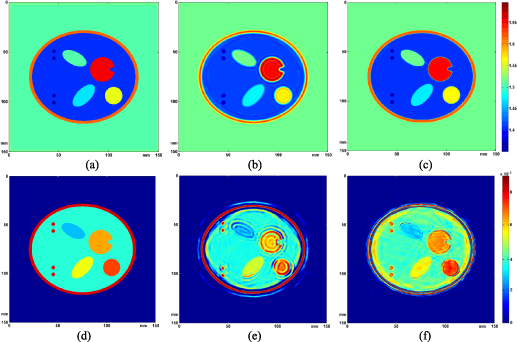
Figure 4. Phantom and reconstructed images: exact speed of sound (a), reconstructed speed of sound,  mm (b) reconstructed speed of sound,
  mm (c), exact absorption factor (d), reconstructed absorption,
  mm (e), reconstructed absorption,
  mm (f).
Download figure:
Standard image High-resolution imageFigure 5(a) shows one-dimensional graphs of the residual functional (4) along the line passing through the initial approximation at  and the exact solution of the problem at
  for the average wavelength
  mm (dashed line) and
  mm (solid line) depending on the parameter
  . The simulation parameters for each
  are calculated as
  ,
,  , where
  are parameters in water, and
  and
and  constitute the exact solution of the problem. Since the calculations were carried out with exact simulated data without measurement errors, the residual functional is zero at the exact solution of the inverse problem. As can be seen from the graph in figure 5(a), the residual functional plot for the wavelength of 5 mm has a bend, which may be associated with a local minimum. Figure 5(a) indirectly shows that the longer the wavelength, the wider the area of convergence of iterative gradient algorithms to the approximate solution.

Figure 5. Plot of the residual functional  for
for  = 15 mm (dashed line), for
  = 5 mm (solid line) (a); reconstructed speed of sound (b) and absorption factor (c) for
  = 5 mm without MSM method.
Download figure:
Standard image High-resolution imageFigures 5(b) and (c) show the reconstruction results of the speed of sound and absorption coefficient obtained via the iterative gradient method using a wideband signal with an average wavelength of 5 mm and an initial approximation  . Given a short wavelength of the sounding pulse, the iterative process started from
  stops at the local minimum of the residual functional, resulting in an incorrect solution.
The reconstructed images shown in figure 4 were obtained to check the convergence of the MSM method to the global minimum. For this reason, some parameters and the tomographic scheme of the model experiment were chosen 'ideal' for tomography problems in order to exclude the influence on the convergence of the MSM method. The number of sources is 24, with six sources located on each side. Wave measurements are taken at each grid point along the perimeter of square  and there are about 100 measurements per wave period in time. The use of broadband sources and receivers with a wide radiation pattern placed at a large number of positions on all sides of the object provide an almost complete set of routes between sources and receivers for sounding the object. This results in high quality image reconstruction.
In addition, all model calculations assumed precisely 'measured' experimental data, i.e. there were no random or systematic errors in the data. The number of iterations of the iterative process was chosen to be greater than 100 at each stage of the MSM method, until the discrepancy stopped decreasing. Of course, such a number of iterations and quality of reconstruction are impossible in processing real experimental data obtained with some error.
Figure 6 shows some results of velocity reconstruction to check the convergence to the global minimum of the MSM method for more realistic values of the experimental parameters. In each experiment in figure 6, a pulse with a central wavelength of 20 mm was used at the first stage of the MSM method, and 5 mm at the second stage. In figure 6(a) the number of sources remains 24, but the step between the measurement points is about 1.5λ ≈ 8 mm and there are about 3–4 measurements per wave period in time. This caused ripples to appear in the image. In figure 6(b), the positions of the measurement points remain as in figure 4, however, the number of sources is reduced to four, with one source located in the center of each side of the square. As can be seen from figure 6(b), this leads to the appearance of artifacts in the image. In figure 6(c), six sources were used, located only on the upper side of the square, but the receivers, as before, were located on all sides of the square. This arrangement of sources results in poor reconstruction at the bottom of the image.

Figure 6. Reconstructed speed of sound: receivers  apart (a), four sources (b), sources only at the top (c).
Download figure:
Standard image High-resolution image
In each experiment in figure 6, the quality of the absorption reconstruction is much worse, so it is not shown. As a rule, to obtain the absorption factor with an acceptable quality, it is necessary to increase the number of iterations by several times compared to the number of iterations required for velocity reconstruction. The reconstruction results for other model and real experiments were presented in [10, 39, 44].
6. Conclusion
The article proves the uniqueness theorem for the solution to the coefficient inverse problem for the wave equation in  with two unknown coefficients: speed of sound and absorption factor.
The original non-linear coefficient inverse problem is reduced to an equivalent system of two uniquely solvable linear integral equations of the first kind with respect to coefficients  and
and  . However, the possibility of reducing the original non-linear problem to a linear one depends on the presence of frequencies close to 0 in the spectrum of the sounding signal. Such frequencies are difficult to obtain in physical experiments. In addition, the solution of the equivalent integral equations of the first kind is a highly unstable problem due to the form of the kernel of the integral operator.
Estimations were made to substantiate the MSM for two unknown coefficients. This justification is based on the idea that for small inhomogeneities at sufficiently low frequencies the non-linear inverse problem approaches a linear problem and the residual functional approaches a convex one. The MSM for solving non-linear coefficient inverse problems is not related to the reduction to a linear problem using a limit approach as  , but assumes solving the inverse problem at sufficiently low but non-zero frequencies
  instead. For small inhomogeneities which are typical, for example, in medical imaging, conducting experiments at such frequencies does not pose significant problems.
The capabilities of the MSM method are demonstrated on a model inverse problem of determining unknown speed of sound and absorption coefficients in some region. The model problem is focused on ultrasound diagnostics of soft tissues in medicine. The presented model problem demonstrates that in ultrasonic tomography the residual functional can have local minima, and therefore the convergence of gradient iterative minimization methods is not guaranteed. The MSM method effectively solved the problem of non-linearity in two stages.
Acknowledgments
The paper was published with the financial support of the Ministry of Education and Science of the Russian Federation as part of the program of the Moscow Center for Fundamental and Applied Mathematics under the Agreement № 075-15-2022-284. The research is carried out using the equipment of the shared research facilities of HPC computing resources at Lomonosov Moscow State University.
Data availability statement
All data that support the findings of this study are included within the article (and any supplementary files).