


Abstract
Conventionally, neutral beam injection (NBI) in tokamaks is controlled via engineering parameters such as injection voltage and power. Recently, the high-fidelity real-time NBI code RABBIT has been coupled to the discharge control system of ASDEX Upgrade. It allows to calculate the NBI fast-ion distribution and hence the properties of NBI in real-time, making it possible to control them directly. We successfully demonstrate control of driven current, ion heating and stored fast-ion energy by modifying the injected beam power. A combined ECRH and NBI controller is also successfully tested, which is able to adjust the heating mix between ECRH and NBI to match a certain desired ion heating fraction at given total power. Further experiments have been carried out towards control of the ion heat flux (i.e. ion heating plus collisional heat transfer between ions and electrons). They show good initial success, but also leave room for future improvements as the controller runs into instabilities at too high requests.
Export citation and abstract BibTeX RIS

Original content from this work may be used under the terms of the Creative Commons Attribution 4.0 license. Any further distribution of this work must maintain attribution to the author(s) and the title of the work, journal citation and DOI.
1. Introduction
Traditionally, neutral beam injection (NBI) in tokamaks is controlled via engineering parameters such as injection voltage and power [1, 2]. For efficient fine-tuning of experiments it would be beneficial to control NBI heating properties directly. Towards non-inductive and advanced operation scenarios [3], it would be helpful to control directly the amount of driven current. The amount of fast-ion content (e.g. the ratio of stored fast ion energy Wfi over the total plasma energy Wmhd) determines if certain mechanisms such as excitation of Alfvén eigenmodes are triggered [4, 5]. Stabilization of ITG turbulence by fast ions even requires certain gradients of their temperatures and densities [6]. Lastly, ion heating, or more precisely the ion heat flux Qi appears to be relevant for the LH-transition [7–9] and transport behavior [10]. For example, matching similar Qi values under varying background plasma conditions might help to conduct better transport experiments.
To allow a more direct control of NBI heating properties, real-time knowledge of the latter must be available. With the development of the RABBIT code [11, 12], this became now accessible: RABBIT is real-time capable while having still a quite high fidelity, e.g. usually good agreement is found [11–13] with the numerically much more heavy TRANSP-NUBEAM [14–17] Monte-Carlo code. RABBIT has recently been integrated as a satellite [18] into the discharge control system (DCS) [19] of ASDEX Upgrade, such that information like the driven current, fast-ion energy and ion heating are routinely available already in real-time [13]. Hence it becomes possible to control these outputs of RABBIT with the control system, and the subject of this paper is the first demonstration of this. RABBIT calculates full radial profiles (e.g. heating power density etc), but for this first demonstration, we focus on controlling scalar quantities, e.g. the total (i.e. volume-integrated) ion heating power or the total current drive (i.e. surface-integrated driven current density).
2. Control of scalar outputs by modifying PNBI
In this section we demonstrate the control of several scalar RABBIT outputs (e.g. NBI current-drive) by modifying the NBI input power PNBI. This is done with a Proportional-Integral (PI) controller, whose controller gains are found beforehand with a simplified model. The ASDEX Upgrade NBI beams can be either switched on or off, but quasi-continuous values of PNBI are achieved with pulse-width modulation. Which beams are used can be programmed by a priority list in the actuator manager [20]. In case of failure of one or more beams, the next ones on the priority list will succeed.
RABBIT was run in steady-state mode, meaning that for each time-step it will instantly calculate the steady-state solution. This means that a delayed response due to changing NBI power on the time-scale of the fast-ion slowing down is neglected. The steady-state mode was used for two reasons: First, at the time of the experiments, the time-dependent mode was not yet robustified for non-equidistant time-steps, as they do occur in our real-time setup where RABBIT is allowed to run as fast as possible [13]. The robustifaction has been carried out in the meantime and is discussed in [13]. Second, this approach might make the controller easier to design and more stable, since we ultimately do want to control and achieve the steady-state solution. If RABBIT would run in the time-dependent mode, the design of the controller will become more challenging, because the delayed response of the RABBIT output to PNBI needs to be taken into account to avoid e.g. over-shoots. This might also make the controller slower, overall.
As final remark, it should be noted that typically the difference between steady-state and time-dependent RABBIT should not be very large, as the average slowing down time ranges from  20–80 ms in our discharges, which is not very large compared to the typical RABBIT time-step of
  15–25 ms and the period of the pulse-width modulation (24 ms). This can be inferred also in this publication: When we will show comparisons of the real-time RABBIT to offline calculations with RABBIT and TRANSP-NUBEAM, the offline calculations for both codes will always be in time-dependent mode.
2.1. NBI current-drive
Figure 1 shows time-traces of the first experiment (#38308) to control the NBI current-drive (NBCD). The scenario is based on a low-density, highly non-inductive scenario. We have programmed an NBCD trajectory which features ramps and a sharp step at the end of the plasma discharge. In between the ramps, there is a longer constant phase, where we want to demonstrate that the controller is able to keep the NBCD constant even under changing background plasma conditions. The latter are emulated by a pre-programmed drop of ECRH power at 4.2 s. Our first attempt, #38308, features some oscillations of the actually achieved NBCD trajectory. This is due to non-optimal controller gains (see table 1), because the beams drove more current than expected. A second attempt with optimized gains (#38310, figure 2) shows then a very good behavior and the target trajectory is met well. This could be automated in the future by calculating the current-drive efficiency with RABBIT, and scaling the controller gains accordingly.

Figure 1. Time traces of #38308. (a) Top: Plasma current, stored plasma energy and safety factor q at 95% of the poloidal flux (i.e.  ). Middle: Line-averaged density for a central and edge interferometer line of sight. Bottom: Heating time traces. (b) NBCD target (as set in the discharge program) in comparison to the achieved value (as calculated by real-time RABBIT).
Download figure:
Standard image High-resolution image
Figure 2. Time traces of #38310. (a) Top: Plasma current, stored plasma energy and safety factor q at 95% of the poloidal flux (i.e.  ). Middle: Line-averaged density for a central and edge interferometer line of sight. Bottom: Heating time traces and total radiated power. (b) NBCD target (as set in the discharge program) in comparison to the achieved value (as calculated by real-time RABBIT) and to offline calculations with RABBIT and NUBEAM.
Download figure:
Standard image High-resolution imageTo cross-check the real-time results we have carried out offline simulations both with RABBIT (in time-dependent mode) and TRANSP-NUBEAM. The offline inputs are more precise as there are much more diagnostics available than in real-time, and even the NBI power signals are less accurate in real-time (see section 3.2).
It should also be noted that the current real-time implementation of RABBIT in the DCS makes the assumption  , where
  means flux-surface average, because the current version of the real-time equilibrium code JANET provides only
  and not
  .
.  is needed to calculate the area elements [13] which are needed to integrate the driven current density into an absolute current. Above approximation hence only affects the current drive output of RABBIT and it should be a quite good approximation. It will be removed with the next upgrade of JANET.
The agreement between offline-RABBIT and TRANSP-NUBEAM is excellent, underlining the high fidelity of RABBIT. The offline calculations are done in time-dependent and the real-time calculation is done in steady-state mode. One can see that the steady-state assumption does not cause strong deviations: A delayed response to the large jump at 7 s is visible, but otherwise, the qualitative temporal behavior is very similar. Overall, both offline calculations are a bit lower than the real-time result (here mostly due to inaccuracies in the real-time Te profile). It is planned to revisit the real-time Te data evaluation and calibration. Since the raw data is coming from the same diagnostic (ECE) it should be possible to further improve the real-time data quality and hence the agreement. But also in the current state, the agreement is still reasonable and hence we can conclude that control of NBCD has been demonstrated successfully.
2.2. Fast-ion stored energy
The fast-ion content has a strong influence on the plasma behavior. Too many fast-ions can trigger MHD instabilities such as Alfvén eigenmodes [4, 5]. Control of these Alfvén eigenmodes, e.g. by reducing their drive by lowered NBI power, is a research topic of its own [21], and the neutron emission calculation by RABBIT could help to determine how harmful the Alfvén eigenmodes are, e.g. by estimating how strong the measured neutrons fall short with respect to the expectation based on a neo-classical fast-ion distribution. On the other side, fast ions can stabilize turbulence [6] if their density and temperature gradient is appropriate. Advanced control schemes might help to tailor the fast-ion profiles to achieve and sustain these high confinement regimes more readily (at least in present-day machines, where most fast ions stem from external heating sources).
For a first controller test, several scalar quantities would be possible, e.g. the volume integrated fast-ion density (potentially also inside a certain radius). Here we chose the fast-ion stored energy, or more precisely its ratio with respect to the total plasma energy, i.e.  . This has the advantage of being a dimensionless quantification of the fast-ion content, while perhaps being more descriptive than e.g. the ratio of particles. Wmhd is estimated by the real-time equilibrium reconstruction based on function parametrization (FP) [22, 23], since JANET does currently not output Wmhd.
Figure 3 shows ASDEX Upgrade discharge #39654. It features a similar requested trajectory with ramps, steps and a constant phase which is well achieved by the controller. However, the response of the controller seems to be a bit slower than in the second NBCD case (figure 2). This is most visible during the large step at 7 s, but also e.g. during the downward ramp (e.g. around 6 s). This suggests to use slightly more aggressive (i.e. larger) controller gains in the future (see table 1 for the used values).

Figure 3. Time traces of #39654. (a) Top: Plasma current, stored plasma energy and safety factor q at 95% of the poloidal flux (i.e.  ). Middle: Line-averaged density for a central and edge interferometer line of sight. Bottom: Heating time traces and radiated power. (b)
  target (as set in the discharge program) in comparison to the achieved value (as calculated by real-time RABBIT (Wfi) and FP (Wmhd)).
Download figure:
Standard image High-resolution imageAn offline RABBIT calculation with more precise inputs (i.e. Wmhd and equilibrium from CLISTE, Te and ne from IDA integrated data analysis [24]) shows a small deviation but overall good agreement. In this case, the deviation seems to originate from missing CXRS real-time measurements: An offline simulation without CXRS data, making the same assumptions of  and zero rotation as in real-time, shows excellent agreement with the real-time simulation. During most of this discharge, core Ti is less than half of Te, such that our real-time assumption of
  is not very good. Nevertheless, since Ti has only a very weak effect on the fast-ion distribution function, the deviations are still quite small and the control experiment can be considered successful.
2.3. Ion heating
The NBI-induced fast-ions slow down in collisions with the background plasma and heat it accordingly. Whether these collisions are happening with electrons or ions determines how strong the electron and ion heating of NBI is. RABBIT calculates radial profiles of both heating densities. For the control experiments, we focus on the volume-integrated heating of ions.
The ion heating controller has been tested for the first time piggy-back at the end of discharges #38134 and #38137. In the first, two power levels of ion heating (with a step) have been programmed into the discharge program and in the second it is a ion heating power ramp. As can be seen in figure 4, both for the ion heating power steps and ramp the target values are matched very well.

Figure 4. First test of the ion heating controller. (a) #38134 two power levels with a step (b) #38137 two power levels with a ramp.
Download figure:
Standard image High-resolution imageIn discharge #38164, we have also tested steeper ramps and a phase where the controller should keep the ion heating constant, while the background plasma changes. As in previously described experiments, this is done by lowering the pre-programmed ECRH power (here at 6.7 s). In figure 5(b) one can see that the real-time measured electron temperature Te clearly drops during that time window. Te has a very direct impact on the distribution of ion and electron heating, because the critical energy Ec, above which fast ions collide dominantly with electrons instead of thermal ions, is given by  in a D plasma with D beams [25–27]. In figure 5(a) we can clearly see that the controller reacts to the dropped Te by increasing PNBI, thus keeping the ion heating constant as requested.

Figure 5. #38164: (a) Test of the ion heating controller in the presence of background plasma variations. A Te variation is induced by lowering the ECRH power and the controller is able to keep the ion heating constant by increasing PNBI. (b) Te as estimated in real-time by RAPTOR.
Download figure:
Standard image High-resolution image3. Control of ion heating and heat flux at constant heating power
In the previous experiments, the ion heating power was matched by only changing PNBI and thus changing the total heating power. For experimental applications, it is much more useful to be able to change only the ratio of ion heating with respect to the total heating power. Since the injection voltage of the beams at ASDEX Upgrade cannot be changed during the discharge, the best way to do this is exchanging ECRH with NBI. ECRH will only heat the electrons, and NBI will be operated at low injection energies to heat ions dominantly.
3.1. Controller setup
The controller output uk (in the kth time-step) will then be a vector of both heating powers. To this end we use the general form of a MIMO (Multi-Input-Multi-Output) controller, which can be written as:


Here, ek
is the error vector in the kth time-step,  is the feed-forward input vector. xk
is the controller state vector, which has no direct physical meaning but can be defined such to match the control goals. A, B, C, D and K are matrices with constants.
is the feed-forward input vector. xk
is the controller state vector, which has no direct physical meaning but can be defined such to match the control goals. A, B, C, D and K are matrices with constants.
In this general form, the controller had already been implemented in the DCS. The values of the vectors and matrices can be configured flexibly by only modifying an xml configuration file, and new controllers of the same type with other parameters can be added flexibly as well.
In our case, we choose the vectors and matrices to be:
This means that effectively we setup a conventional PI controller for PNBI in the first row, while the second row simply evaluates the boundary condition  .
.  can be the raw injected NBI power signal
  , or the NBI heating power as calculated by RABBIT
  . The latter accounts for NBI power losses (e.g. due to shine-through and promptly unconfined orbits) to ensure that the total effective heating power (i.e. after subtraction of losses) is kept constant. We have tested both settings in the following. Δt is equal to the time step, i.e. the cycle time of the DCS which is 1.5 ms in all discharges of this publication. The last term in equation (4) is there to counter-act integral windup in the case of saturating actuators (only then
  , since
  ), but it is irrelevant for our purposes because it is always zero during the experiments in this publication.
3.2. Ion heating
To test this new control scheme, we chose a very low density scenario (core densities around  ) which was designed to study LH transitions. This scenario is interesting, because we can connect our control experiments with physics of the LH transition, namely the established theory that the LH transition is triggered by a threshold in (surface integrated) ion heat flux Qi, rather than total heating power [7–9].
The (volumetric) ion heat-flux density qi is given by the ion heating density plus the equipartition power density (i.e. collisional heat transfer between electrons and ions):
Hereby, temperatures are in keV, densities in  ,
,  is the Coulomb logarithm, Zj
and Aj
are charge and mass numbers of the ion species j, respectively, and the result is in MW m−3 [28–30]. Qi and ion heating are then volume integrals of qi and pion, respectively, and are both measured in Watts.
is the Coulomb logarithm, Zj
and Aj
are charge and mass numbers of the ion species j, respectively, and the result is in MW m−3 [28–30]. Qi and ion heating are then volume integrals of qi and pion, respectively, and are both measured in Watts.
In low density plasmas, the coupling between electrons and ions (i.e. the equipartition term) is weak and hence one can modify the ion heat flux by changing the ion heating. In a high density plasma, this would not be possible because even for pure electron heating there would be a considerable ion heat-flux due to collisional heat transfer from the electrons to the ions.
Hence, it should be possible to design discharges that start with 100% electron heating still in L-mode and will transit into H-mode while ramping up the ion heating ratio at constant total power. A few setup discharges have been carried out to identify the parameter window where this is possible.
Figure 6 shows the first test of such a discharge. The plasma is initially heated with two gyrotrons, staying in L-mode. At 3.0 s, an ion heating ramp is programmed while keeping the total heating power constant and the LH transition is triggered at 4.3 s. The controller achieves the ion heating ramp almost perfectly. The total power is, however not fully constant.

Figure 6. Time traces of #38307. (a) Overview plot in the same style as figure 1(a). Transition from L- to H-mode is indicated with a grey vertical line. (b) Results of the control experiment. Target traces of ion heating (ramps) and total power (constant line) in comparison to the achieved values. For the total power,  is set to
  (see text). For comparison, offline calculations with TRANSP-NUBEAM (i.e. using more diagnostics than available in real-time) of the ion heating and ion heat flux Qi are shown.
Download figure:
Standard image High-resolution imageIn phase (b), this is simply due to saturation. We have demanded too much ion heating, and the ECRH power cannot become negative. The controller here decides to match the ion heating time-trace, sacrificing to keep the total power constant. The opposite behavior would be better and more stable, i.e. to just keep the total power constant with 100% NBI. This can be programmed easily in future experiments by clipping the NBI power to the maximum total power. Such a clipping feature was not available in the DCS at the time of the experiment, but has been included in the mean time. Even more elegantly, the same could also be achieved in the future by setting matrix K in equation (4) to
ensuring that saturation in ECRH power will be compensated with opposite sign in the NBI power request and vice versa.
In phase a) the total power is not constant due to uncertainties in the real-time NBI power signals during pulse-width modulation. As one can see in figure 7, the NBI system reacts with a delay to the modulation requests sent by DCS. The delay is longer for switch-on than for switch-off, resulting in a different duty cycle percentage. To solve this, new signals for all eight NBI beams with the actual NBI power have been routed and made available in the DCS.

Figure 7. (a) #38307: Comparison of requested (black lines) and actually delivered heating powers. The ECRH powers match well but there is an inaccuracy for NBI powers. (b) #39653: Reason and solution for the inaccurate real-time NBI power signals. The NBI power (offline data shown in black) reacts with a delay to the requests (blue) sent by DCS, resulting in a lower duty-cycle percentage. To take this into account, a new signal (red) has been made available in real time, which matches reasonably well with the offline data.
Download figure:
Standard image High-resolution imageFigure 8 shows a subsequent repeat of the experiment.  is now set to
  , where as in the previous attempt it was set to
  . The ion heating target is again matched very well, and the constancy of the sum of ECRH power and effective NBI heating power (i.e. after subtraction of RABBIT-calculated losses) is better than the constancy of ECRH + NBI power in the previous attempt. However, it is still not perfect and as one can see in figure 9. This time, it seems to be mainly caused by uncertainties in the real-time ECRH power. For example, the actuator manager of the DCS assumes that each gyrotron has the same power of 700 kW whereas in this discharge the real power of the gyrotrons was in the range of 500–800 kW. For example, gyrotron 2 and 3, which were active from 3–5.8 s delivered both 800 kW while the later replacements 4 and 5 delivered 800 kW and 500 kW, respectively (comp. figure 9(b)). These deviations from the constancy of power could be improved further in future experiments, by configuring the actuator manager with the expected power from each gyrotron.

Figure 8. Time traces of #39653. (a) Overview plot in the same style as figure 1(a). Transition from L-mode to I-phase is indicated with a grey vertical line. (b) Results of the control experiment. Target traces of ion heating (ramps) and total power (constant line) in comparison to the achieved values. In this discharge the effective heating power (red curve), i.e. after subtracting NBI losses as computed by RABBIT, is supposed to be kept constant (i.e.  is set to
  ). For comparison, offline calculations with TRANSP-NUBEAM (i.e. using more diagnostics than available in real-time) of the ion heating and ion heat flux Qi are shown.
Download figure:
Standard image High-resolution image
Figure 9. (a) #39653: Comparison of requested (black lines) and actually delivered heating powers. Here, the NBI powers match well (thanks to the newly installed real-time NBI power signal), but an inaccuracy is visible in ECRH powers. This is caused by the DCS assuming 700 kW for each gyrotron, while the actual gyrotron powers deviated in this discharge (as shown in (b)).
Download figure:
Standard image High-resolution imageTo validate the real-time calculations of RABBIT we have again carried out offline calculations with the TRANSP-NUBEAM code. They are drawn with orange curves in figures 6(b) and 8(b) and the agreement with real-time RABBIT is good in #38307 and excellent in #39653 (which had the improved NBI power signals). This indicates that we controlled the ion heating correctly and that the improved NBI power signals have also improved the controller accuracy. In summary, control of the ion heating ratio at constant total heating power was demonstrated successfully.
3.3. Ion heat flux
Now we want to move one step further and try to control the ion heat-flux Qi. As mentioned in equation (6), it is given by the sum of the ion heating and the equipartition term. This control scheme is more challenging, because the latter term is rather self-organized by the plasma and cannot be controlled from outside.
For the previous discharges, we have calculated Qi already and plotted it with yellow curves in figures 6 and 8. One can see that while controlling the ion heating, we have also modified the ion heat flux in a similar fashion: Surely, Qi cannot go to zero, because even at  , there is a residual energy transfer from the electrons to the ions. But this Qi baseline is low enough and eventually, the ion heating ramp coincides with a Qi ramp. This means that the equipartition term is weak enough (due to the low density plasma scenario) to allow an attempt to control Qi.
To evaluate the equipartition term, we need profiles of ne, Te and Ti. For the first two, measurements are readily available in real-time at ASDEX Upgrade with interferometry and electron cyclotron emission (respectively). The real-time profiles are then estimated by RAPTOR (taking into account the measurements and a transport model) [31]. For Ti, unfortunately no real-time diagnostic (e.g. CXRS) is available, and the RAPTOR assumption of  is too simplified for our application. To overcome this, we estimate the energy of the thermal ions by taking the plasma energy Wmhd as determined by the real-time equilibrium function parametrization (FP) [22, 23] and subtracting all other plasma species:

Here, w stands for energy densities and the energy W is obtained by volume integration of the w-profiles. The parallel and perpendicular fast-ion energy densities  and
and  are obtained by the RABBIT code and the rotational energy density wrot is assumed simply zero (due to lack of real-time rotation measurements). This is a good approximation especially in cases of low NBI power (and hence torque input), e.g. in #39653 the value of
  does not exceed 0.7%.
Then, a mock-up Ti profile is calculated to match the ion energy  . Here, we assume one main ion species (i.e. deuterium) with thermal ion density
  and one impurity species (i.e. carbon) with density nimp. The latter approach is justified because high-Z impurities (such as tungsten) do not contribute significantly to the plasma dilution (due to their very low concentrations), and carbon is a suitable representative for the various low-Z impurities. The mock-up Ti is created as follows:
ρtor refers to the square-root of normalized toroidal flux. Outside of  , we assume
  and consequently zero equipartition, because otherwise, e.g. when using a simpler approach such as
  , the equipartition will get very high in this region and the Qi value can become arbitrary as a consequence. Inside of
  we use Te as a basis and subtract a linear function where the constant prefactor is calculated such to match Wion.
The results of this approach for discharge #39656 are shown in figures 10 and 11. It can be seen that in this discharge, it works surprisingly well and values of core Ti are in very good agreement with offline CXRS data, capturing correctly even the large increase in Ti at 5.5 s. Also the profile shape estimates are reasonable, although in situations where  a nonphysical reversal of the Ti-gradient appears due to our approach. Even though this has no strong implications for our application, this can be improved in future experiments.

Figure 10. Comparison of the real-time Ti estimate (based on Wmhd) with offline CXRS (Charge Exchange Recombination Spectroscopy) measurements for three time points of discharge #39656. Also shown is the real-time estimate of Te by RAPTOR (based on ECE measurements).
Download figure:
Standard image High-resolution image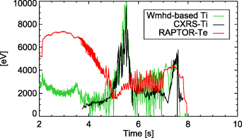
Figure 11. #39656: Time traces of temperature values in the plasma core.
Download figure:
Standard image High-resolution image
Qi is then estimated based on equation (6) and a subsequent volume integration (up to  ). Hereby, we assume the Coulomb Logarithm,
  , to be 16. In the sum over ion species j we consider one thermal ion species (deuterium) and one impurity species (carbon). The impurity density is given by the RAPTOR Zeff estimate (which is hardwired to 1.5 due to lack of diagnostics—this is a reasonable assumption since AUG is a tungsten device). The thermal ion density is given by subtracting impurities and fast-ions (as calculated by RABBIT) from ne. Figure 12 shows a comparison of the real-time Qi estimate with an offline TRANSP calculation (i.e. including CXRS measurements for Ti) for discharge #39656 and the agreement is very good.

Figure 12. Time traces of #39656. (a) Overview plot in the same style as figure 1(a). Transitions from L-mode to I-phase to H-mode are indicated with a grey vertical lines. (b) Results of the control experiment. Target traces of ion heat flux Qi (ramps) and total power (constant line) are shown in comparison to the achieved values. For the total power,  is set to
  (see text). It has been checked that the slight mismatch in total power stems again from uncertainties of the assumed ECRH power in the DCS actuator manager (comp. section 3.2). Offline calculations with TRANSP-NUBEAM (i.e. using more diagnostics than available in real-time, in particular CXRS Ti) of the ion heat flux Qi are shown and they match well. In addition, the ion heating from RABBIT is drawn.
Download figure:
Standard image High-resolution image
Figure 12 shows results of the first experiments to control the ion heat flux Qi. The programmed target trajectories and plasma scenario are similar as for the ion heating case. The controller worked quite well in the initial phase of the ramp. At the beginning (3 s), the controller just stays at 100% ECRH heating, because it cannot lower Qi anyhow. After ≈3.5 s the controller reacts to the increasing target-Qi by exchanging ECRH power with NBI power. This works quite well for about a second, when oscillations start to appear that get worse over time, and also lead once again to an over-shoot of NBI power, hence also violating the constancy of total power. This leads to a strong density increase which increases the equipartition term, and hence makes further Qi control impossible.
We make the following suggestions for improvement in subsequent experiments: First, one should request less Qi. Second, the recently added feature of clipping the NBI power should be activated here too, to ensure constancy of total power also in situations where the controller is at 100% NBI heating. This would prohibit also the density increase which leads to a plasma state where Qi control is no longer possible. To mitigate the oscillations, one could thirdly implement low-pass filters on the quantities entering into the equipartition term (i.e. Te, Ti and ne.) In our analysis we could not identify a single source for the oscillations. Ti does have the strongest oscillations in the phase around 4.6 s, but e.g. also Te data shows oscillations, which could partly be induced by the controller oscillating between high ECRH and high NBI heating. Lastly, improvements in the Ti estimate would be very beneficial. In attempts to implement the first two of the above suggestions and repeat the experiment, the Ti estimate was less accurate than in the example above (without changing anything about the Ti estimate). Hence it is currently not in a very reliable state, and it is unclear if the current method can be robustified, because Wmhd comes with uncertainties, which get worse as we subtract all other plasma species from it: We essentially subtract two large numbers from each other, and the remainder determines then Ti, consequently with a high uncertainty. The ideal solution to this issue would be a real measurement of Ti in real time, e.g. through real-time CXRS.
In conclusion we can however state that the proof of principle of a Qi controller was already successful. With additional work, it could be robustified and made ready for experimental applications.
4. Summary, conclusion and outlook
RABBIT is a real-time capable high-fidelity NBI code which has been recently coupled to the DCS of ASDEX Upgrade and runs now routinely. Therefore knowledge of the NBI fast-ion distribution and the related heating and current-drive properties are known in real time. This allows to replace the traditional control of NBI via engineering parameters by programming directly in the discharge program the requested properties.
Concretely, control of driven current, ion heating and stored fast-ion energy has been demonstrated successfully by modifying the injected beam power. For the ion heating, a more advanced controller has been developed which is able to adjust NBI and ECRH powers to match a requested ion heating ratio at a given total heating power. This is done via an existing implementation of a generic Multiple-Input Multiple-Output controller which was already implemented in the DCS.
The gains for these controllers are found with simplified models beforehand the discharge. Input to these models is e.g. how much current-drive is expected from each beam (for the current drive controller). Since this is scenario-dependent, the gains, in principle, must be recalculated for each plasma scenario. If a more routine use of these controllers is desired, it would be therefore beneficial to automate this, e.g. by letting RABBIT calculate the expected current-drive efficiency and hence adjusting the gains.
First steps towards control of the ion heat flux Qi (i.e. ion heating plus collisional heat transfer between electrons and ions) have been taken. Due to a lack of real-time Ti measurements, an estimated Ti profile has been implemented based on Wmhd from the JANET equilibrium code and a subsequent subtraction of all other plasma species that contribute to it. While not being fully robust, it yielded good results at least in one discharge where we have attempted a Qi control. The latter has worked initially well, leading only to instability at high Qi requests. To improve this, we propose in future experiments a lowered Qi request, clipping of NBI power, low-pass filters to reduce oscillations and a more robust Ti estimate.
Such a robustified Qi controller could be used to study alpha-particle heating by emulating it with auxiliary power [32]. In this way, the behavior of the plasma including self-generated fusion heating, which depends non-linearly on the plasma temperature (e.g. lower temperatures causing also lower heating), could be investigated already in present-day devices.
Acknowledgment
We thank N. den Harder, C. Hopf and J. Thalhammer for their help in providing the improved real-time NBI power signals. We also thank A. Bock and M. Reisner for providing a reference scenario for the current drive control discharges and we thank E. Fable for discussions about and supplying motivation for the Qi controller. We also thank M. Cavedon for his help identifying the LH transitions. We are grateful to P.A. Schneider for allowing to do the first tests of the ion heating controller piggy-pack in his discharges. This work has been carried out within the framework of the EUROfusion Consortium, funded by the European Union via the Euratom Research and Training Programme (Grant Agreement No. 101052200 — EUROfusion). Views and opinions expressed are however those of the author(s) only and do not necessarily reflect those of the European Union or the European Commission. Neither the European Union nor the European Commission can be held responsible for them.
Appendix: Overview of discharges and controller gains
Table 1. Overview of discharges (in the order they appear in this publication) and proportional and integral controller gains, Kp and Ki, respectively.
| Discharge | Kp | Ki | Controller mode |
|---|---|---|---|
| 38308 | 25 W A−1 | 750 W (As)−1 | INBCD |
| 38310 | 10 W A−1 | 300 W (As)−1 | INBCD |
| 39654 | 2.5 MW | 80 MW s−1 |

|
| 38134 | 1.0 | 30 s−1 | Pion |
| 38137 | 1.0 | 30 s−1 | Pion |
| 38307 | 1.0 | 30 s−1 |
Pion at const. 
|
| 39653 | 1.0 | 30 s−1 |
Pion at const. 
|
| 39656 | 1.0 | 30 s−1 |
Qi at const. 
|