

Abstract
Landscape complexity promotes ecosystem services and agricultural productivity, and often encompasses aspects of compositional or configurational land cover diversity across space. However, a key agricultural diversification practice, crop rotation, extends crop land cover complexity concurrently across space and time. Long-term experiments suggest that complex crop rotations can facilitate yield increases in major crops. Using a compiled county-annual panel dataset, we examined whether yield benefits of crop rotational complexity were apparent on a landscape scale in the conterminous US for four major crops between 2008 and 2020. We found that the benefit of rotational complexity was only apparent for cotton and winter wheat, and that the benefit for wheat was driven by one region. Corn exhibited the opposite pattern, wherein higher yields were consistently obtained with lower rotational complexity, while soybean yield appeared relatively insensitive to rotational complexity. Effects of rotational complexity were sometimes influenced by agrochemical usage. Positive effects of rotational complexity were only apparent with high fertilizer for soybean and wheat, and with low fertilizer for cotton. Corn yield in high-complexity, low-yielding counties appeared to improve with high fertilizer inputs. For the overwhelming majority of acres growing these major crops, crop rotation patterns were quite simple, which when combined with the short time span of available data, may explain the apparent discrepancy between long-term experiments and nationwide data. Current demand and incentives that promote highly intensified and specialized agriculture likely hinder realization of the benefits of rotational complexity for production of key crops in the US. Increasing rotational complexity where major crops are grown thus remains an underutilized approach to mitigate landscape simplification and to promote ecosystem services and crop yields.
Export citation and abstract BibTeX RIS

Original content from this work may be used under the terms of the Creative Commons Attribution 4.0 license. Any further distribution of this work must maintain attribution to the author(s) and the title of the work, journal citation and DOI.
1. Introduction
Complex landscapes enhance biodiversity and promote a variety of ecosystem services that contribute to agricultural productivity [1, 2]. Yet, agricultural transformations over the past century have greatly simplified landscape composition and configuration [3, 4]. Landscape simplification has many associated consequences, including declining water quality, increased insecticide use, weakened pollination, disrupted pest regulation, and reduced resilience to environmental change [5–9]. Efforts to increase complexity in agricultural landscapes, such as the addition of prairie strips to crop fields, for example, have shown promise to reverse some of these effects without compromising yield [10, 11]. Nevertheless, rising food, fiber, and fuel demand warrants strategies to simultaneously improve landscape complexity and agricultural production without replacing cropland.
One approach to enhance landscape complexity that does not involve replacing cropland with non-agricultural land uses is to increase the diversity of crops grown in a landscape. Crop rotation is one such agricultural practice that has been implemented for millennia to increase the diversity of crops grown in a field over time [12, 13]. Beyond nominal species diversity, crop rotation increases the functional diversity of agricultural land cover by sequentially introducing annual or perennial crops, cereals, nitrogen fixing species, and crops with floral displays visited by pollinators and natural enemies. Crop rotation also increases variance in the timing, type, and intensity of management interventions, which can disrupt agricultural pest life cycles [14]. At a landscape scale, the temporal variation introduced by crop rotation practiced across many farms results in greater complexity across space. Such diversification of crops over space and time contributes to the resilience of agricultural systems and their nutritional output to extreme weather and market disruptions [15–18] and is recognized by many farmers as a climate change adaptation strategy [19].
Benefits of rotational complexity at a field scale are numerous. Rotational complexity boosts soil organic matter and total soil carbon [20–24], improves soil water holding capacity and water use efficiency [25, 26], reduces flood risk [27], and stimulates nitrogen cycling [28]. Diverse crop rotations contribute to weed suppression and can be as profitable as conventional herbicide-based weed management strategies [14, 29, 30] while reducing freshwater pollution from agricultural runoff [31]. Importantly, rotational complexity increases yields [16, 32, 33] and yield stability [34, 35]. However, whether these field-scale benefits are ultimately translating to observable increases in yields at a landscape scale is uncertain.
Rotational complexity includes components of crop richness and crop turnover across time. Previous studies have identified positive effects of land cover diversity on agricultural productivity at landscape scales [36, 37], but have not explicitly considered rotational complexity. Socolar et al (2021) designed a crop rotational complexity metric to account for these combined effects of crop richness and turnover while further rewarding rotations that retain perennial crops for multiple years and used it to describe and predict drivers of highly simplified corn- and soybean-dominated crop rotations in the US Midwest. Here, we assess whether increased rotational complexity has positive effects on agricultural productivity at a landscape scale. We extend examination of crop rotational complexity to four major crops (corn, cotton, soybean, winter wheat) and the entire contiguous US in 6 year intervals between 2008 and 2020. We then aggregate crop rotational complexity data to a county level and combine it with county-level crop yield estimates to test for associations while accounting for variation in other biophysical factors known to influence crop yields. We finally repeat this analysis at a regional scale and while accounting for potential interactions with agrochemical inputs to examine context dependency of the effects of rotational complexity.
2. Methods
2.1. Data
We constructed panel datasets merging county-level yield estimates from the USDA National Agricultural Statistics Service (NASS) Survey with seasonal sun, soil, and water characteristics for US counties cultivating corn, soybean, (upland) cotton, and (winter) wheat from 2008 to 2020. Together, these crops dominate US agriculture, covering 49% of agricultural land in the US [38]. We constructed three county-season weather indicators—growing degree days (GDDs), stress degree days (SDDs), and total precipitation—from gridded daily 4 km temperature and precipitation data provided by the PRISM Climate Group (2004) [39]. For each indicator, we defined season duration using the spatially explicit, crop-specific planting and harvesting dates provided by Ramankutty et al [40]. GDDs—an indicator of cumulative temperature exposure—are the sum of mean daily temperatures above a crop-specific threshold over the crop's growing season [41, 42] 4 . To model the effects of heat stress on plant growth, we also computed a metric of growing season heat exposure called SDDs which we define as complementary to GDDs: the total accumulated degrees above the maximum GDD temperature threshold (30 °C for corn and soy, 35 for wheat, and 37.8 for cotton), calculated on a daily basis. Total precipitation is the sum of precipitation (in millimeters) throughout the growing season. We also collected data describing the percent of a county's agricultural land irrigated from the USDA NASS [43]. When this data was unavailable, we replaced missing values with linearly interpolated estimates from the MiRAD project [44] standardized by agricultural extent estimates derived from the USDA's Cropland Data Layer (CDL). Because the county-annual scale is the highest spatiotemporal resolution at which agricultural yields are reported for the entire US, all gridded data were averaged to the county-annual scale.
In addition to these seasonal weather indicators, we extracted to the county level an indicator of the suitability of a region's soils to the cultivation of corn provided by the Gridded Soil Survey Geographic (gSSURGO) dataset, the highest accuracy and finest spatial resolution dataset available for US soils [45]. This indicator, the National Commodity Crop Productivity Index (NCCPI), integrates soil chemical properties, soil water properties, soil physical properties, soil climate properties, soil landscape properties to generate a 'crop productivity score' that ranges from 0.01 (low productivity) to 0.99 (high productivity) [46]. To align this gridded dataset with the county-level yield data, we computed the average productivity score of soils across each county.
We quantified the complexity of crop rotation using the rotational complexity index (RCI) described by Socolar et al (2021) according to the equation:
where n is the number of crop types,  is the turnover in crop types from year to year,
  is the turnover of crop types every two years, and
  is the number of times perennial crops (e.g. alfalfa and pasture) are planted back to back (i.e. lack of turn over in crop types is not penalized when those crops are perennial, due to the benefits they provide for soil health). RCI thus combines information about crop richness and crop turnover to represent the overall complexity of crop rotation in a given location over a given time span. Examples of observed crop rotations that represent above average, average, and below average rotational complexity can be found in table S1.
Crop land cover data was obtained at 30 × 30 m resolution from the USDA NASS CDL (https://nassgeodata.gmu.edu/CropScape/), which provides complete coverage of the conterminous US back to 2008. To reduce the impact of land cover classification (omission and commission) errors on RCI calculations, we aggregated the data to 150 × 150 m resolution, reclassifying using the mode of land cover classes. For each focal crop, we then computed RCI for eight six-year intervals between 2008 and 2020 (2008–2013, 2009–2014, etc) for any 150 × 150 m pixel that contained the focal crop in at least one of the years in the six-year time series. Finally, to facilitate comparison of RCI and county-level yield estimates, we took the average of RCI among pixels within each county.
2.2. Models
We employed hierarchical Bayesian spatiotemporal models to isolate the interactions between rotational complexity and agricultural production (yields, measured in bushels per acre 5 ). This flexible modeling approach allowed us to account for well-established non-linearities in the interactions between biophysical factors and yields [47, 48] and control for spatial autocorrelation in yield which might otherwise bias estimates [49, 50]. All models were run using the R-INLA package [51]. The model takes the generic form:
where i indexes counties and t indexes year (2013–2020). Models were run for four crops (corn, cotton, soybean, and wheat). The matrix of Controls includes any temporally varying county-level agricultural system attributes known to influence yields, modeled as linear effects, in this case the percent of a county irrigated and the percent of a county's total land area in agricultural production. The County term refers to conditionally auto-regressive spatial random effects at the county-scale. County-level random effects are modeled using a Besag–York–Mollie spatial dependency model that includes both random effects and county-level intrinsic conditional autoregressive structured residuals between counties. This approach accounts for both random variation in yield across counties and the fact that observations from neighboring counties exhibit higher correlation than more distant regions. The county-level random effects capture time-invariant factors associated with a county that influence yield. The Year term is a dummy variable that controls for space-invariant factors that may influence yields in a particular year such as major market or policy changes. The RCI term refers to the main independent variable of interest: the RCI. Note that unlike the other variables which describe observations for a specific county-year, RCI describes crop rotations over the six-year period before the year in which the other variables were measured (i.e. RCI for 2013 reflects the RCI computed from 2008 to 2013, with the other variables in the model from 2013). TP, GDD, SDD and SOIL refer to the climate variables of total precipitation, GDDs and SDDs and to the crop-specific metric of soil suitability respectively. The climate and soil indicators and RCI employ a latent random-walk model where values were binned into 15 quantiles to avoid over-fitting. Penalized complexity priors were employed for all non-linear effects [52]. For the linear controls, we used Gaussian priors with a mean of zero and precision of 1 × 10⁻⁷.
For each crop, we included counties in which more than 5% of agricultural land was cultivated in that crop, in which more than one yield observation was provided by the USDA over our period of interest, and in which more than 5% of total land area was in agricultural production. We also ran regional models in which we divided the national sample of counties into their farm resource regions (FRRs) to test for regional differences in the effects of RCI on yields (figure 1). We tested model sensitivity to rotation duration by examining the effects of a 10 year rotation (figure S7) and the effects of an interaction between RCI and county-level fertilizer use (figure S8). Model results were robust to these specifications. For each iteration of the models, we evaluated model performance using the widely applicable information criterion (WAIC), mean squared error, Bayesian R2 and the conditional predicate ordinate which evaluates model fit using a leave-one-out cross-validation technique (table S2).
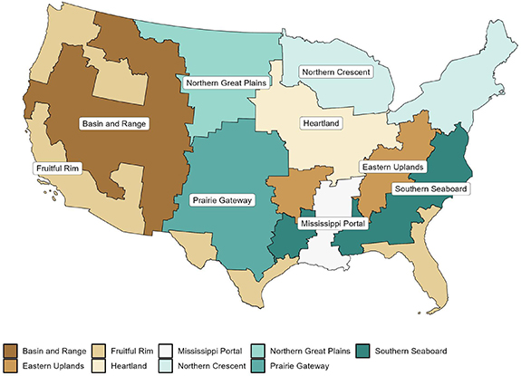
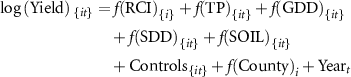
Figure 1. USDA farm resource regions.
Download figure:
Standard image High-resolution image3. Results
3.1. Spatial patterns of rotational complexity in the US
Across crops, rotational complexity (RCI) tends to be lower in high-yielding agricultural regions (figure 2). For example, in the Heartland, a region regularly reporting the highest corn and soybean yields in the US, RCI values reflect simplified rotations of only corn and soybean. As corn and soybean yields decrease along the periphery of the Heartland, crop rotations become increasingly complex and include additional crops such as winter wheat (see table S1 for sample rotations at different RCI values). One exception to this pattern is in the Prairie Gateway, where the rotational complexity for cotton and wheat appears to be influenced by the boundaries of the High Plains Aquifer (figure S3), with simpler cropping patterns (primarily monoculture wheat) occurring in low-yielding regions outside of aquifer boundaries while a wider variety of crops are grown within the aquifer bounds (figure S19). These low-yielding and rotationally simple regions also exhibit strong temporal variation in rotational complexity (figure 2(c)). Nationally, there are no significant differences in rotational complexity across crops (figure S1, table 1); however, within many regions across-crop RCI differences reflect regional specialization—with dominant, high-yielding crops exhibiting simpler rotations than less dominant crops. For example, in the Heartland, rotational complexity for corn and soybean is significantly lower than for wheat, while in the basin and range, a region in which wheat is a dominant crop, wheat exhibits lower rotational complexity than corn (figures S2 and 2(b)).
Figure 2. (A) Standardized average yields, (B) average rotational complexity index, and (C) an indicator of the temporal variability of RCI, the coefficient of variation of RCI for counties over the period from 2013 to 2020 for corn (n = 1670 counties), cotton (n = 340), soybean (n = 1442) and wheat (n = 557).
Download figure:
Standard image High-resolution imageTable 1. Descriptive statistics for crop-specific estimates of RCI.
| Crop | Min. RCI | Max. RCI | Mean RCI | SD RCI |
|---|---|---|---|---|
| Corn | 1.023 | 4.006 | 2.643 | 0.359 |
| Cotton | 0.490 | 3.760 | 2.558 | 0.540 |
| Soybean | 1.124 | 3.887 | 2.514 | 0.325 |
| Wheat | 0.508 | 3.580 | 2.772 | 0.556 |
3.2. Rotation types
The most common rotation type in corn, cotton, soybean, and winter wheat growing areas across the contiguous US is an annually alternating corn–soy rotation, with variants with either two consecutive years of corn or two consecutive years of soy before alternating being the second and third most common rotations (figures 3 and S18). These three rotations cover more than 5% of the entire area of the US, about 12.5% of all US farmland [53] and more than 40% of all US cropland. Notably, four of the top 15 most common rotation patterns across the country, accounting for ∼8.5% of US cropland, do not actually involve rotating crops at all. These are simply monocultures of corn, cotton, soybean, and winter wheat, where the same crop is planted in the same field in at least six consecutive years. In addition, most crop rotations involve only two to three crops or one to two crops along with a fallow period. The most common rotation including four crops across the nation is a sunflower–spring wheat–winter wheat–corn rotation which covers less than 0.02% of the area in the contiguous US or about 0.04% of all US farmland and ∼0.14% of all US cropland.

Figure 3. Dominance of rotation types in corn, soybean, winter wheat, and cotton growing areas across the country by percent of cropland in the contiguous US in each rotation between 2008 and 2020. 'Mostly' indicates that the crop was grown in at least four out of six years.
Download figure:
Standard image High-resolution imageCrop rotations vary by region, and there is notable variation within regions (figure S20), but rotational complexity remains relatively simple in the majority of each region (figures 4, S9–17). The most common rotation differs across regions but in all regions the most common rotation includes only one or two crops, and in three out of nine regions (Prairie Gateway, Mississippi, Southern Seaboard) the most common rotation includes at least four years of the same row crop in a six-year period (figure S4). Only the Northern Great Plains region includes one four-crop rotation pattern in the top 15 most common rotations by region, while the Mississippi Portal includes only monoculture and two-crop rotation patterns in the top 15 most common rotations (see SI for a more detailed discussion of regional differences).
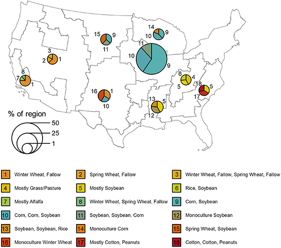
Figure 4. Top three most common rotations in corn, cotton, soybean, and winter wheat growing areas between 2008 and 2020 by farm resource region. Symbol size corresponds to the percent of the total region area covered by that crop rotation pattern. 'Mostly' indicates that the crop was grown in at least four out of six years.
Download figure:
Standard image High-resolution image3.3. Rotational complexity and yield
Model performance was strong for each crop, with Bayesian R2 consistently above 0.7 (table S2). Yields of wheat, and to a lesser extent cotton, increased with increasing rotational complexity (figure 5). The opposite pattern was observed for corn yields, which tended to decrease with increasing rotational complexity. Soybean yields appeared insensitive to changes in rotational complexity (figure 5).

Figure 5. Functional response curves of log corn (n = 10 284 county-years), cotton (n = 2064 county-years), soybean (n = 9268 county-years), and wheat (n = 2875 county-years) yields to the six-year rotational complexity index (RCI). A value of 0 indicates the RCI is at the sample mean while a value of 1 indicates the metric is one s.d. above the sample mean. Solid lines represent the posterior median effect; colored ribbons indicate the 95% credibility limits.
Download figure:
Standard image High-resolution imageWe further examined variation in rotational complexity effects among FRRs where each major crop was well-represented. Decreases in corn yield with increasing rotational complexity were most evident in the Northern Great Plains and Prairie Gateway regions, although slight negative relationships were also evident in the Heartland and Mississippi Portal regions as well (figure 6(a)). In contrast, soybean yield remained relatively insensitive to rotational complexity across FRRs (figure 6(b)). This analysis also revealed that increases in wheat yield with increasing rotational complexity were driven by the Fruitful Rim, while no relationship was apparent in the Northern Great Plains or Prairie Gateway (figure 6(c)). Regional models for cotton yield could not converge due to the relatively narrow distribution of cotton production in the US, preventing further dissection of cotton yield and rotational complexity relationships among FRRs.

Figure 6. Regional effects of rotational complexity on log yields for each crop. Note that the sample size within farm resource regions was too small for cotton for models to converge.
Download figure:
Standard image High-resolution image
We also explored potential interactions between rotational complexity and agricultural chemical inputs (fertilizer, fungicides, herbicides, and insecticides), seeking to assess to what extent effects of rotational complexity were masked in highly intensified agricultural systems. For example, might highly productive agricultural systems exhibit lower rotational complexity because they are relying heavily on external inputs with high costs to achieve yield gains? Overall, relationships between rotational complexity and crop yield did not qualitatively change with the inclusion of this interaction. However, we did observe that the dampening effect of rotational complexity on corn yield was mitigated under high agricultural chemical inputs (figure S8). The positive effect of rotational complexity on wheat yield was also more apparent under relatively high agricultural chemical inputs (figure S8(d)). Broad overlap among 95% credible limits precluded confidence in the interactive effects of rotational complexity and agricultural chemical inputs on cotton and soybean yields. However, we note that positive effects of rotational complexity were only apparent with high fertilizer for soybean and with low fertilizer for cotton.
4. Discussion
Our findings suggest that in the most important regions for the cultivation of corn, cotton, soybean and wheat, crop rotations remain fairly simple. This likely reflects the strong incentives—from federal incentive programs to economics of scale to better market access for regionally dominant crops—that producers face to maintain simplified operations in high yielding regions. Nationally, there are no significant differences in rotational complexity across crops; however, significant differences in rotational diversity across crops exist within major agricultural regions. These regional differences also indicate that dominant crops (e.g. corn and soybean in the Heartland, cotton in the Mississippi Portal, or wheat in the basin and range) are more likely to be cultivated in simpler rotations. These patterns indicate that there is still great potential to increase the rotational complexity for major commodity crops in dominant agricultural regions.
Overall, the most dominant cropping patterns for corn, cotton, soybean, and winter wheat growing areas consist of monoculture or two crop rotations. A corn–soybean annually alternating rotation and two years of corn followed by one year of soybean are more than four times and two times more prevalent, respectively, than the next most common rotation pattern across the country. Although more complex three and four crop rotations (e.g. sunflower, spring wheat, winter wheat, corn) are observed in some regions, in terms of the area to which they apply, they are still more of an exception than the rule. Generally, rotations seem to be most complex in areas where growing crops is most challenging due to biophysical conditions such as the Northern Great Plains. Prior work has shown that rotational complexity tends to be lower in areas where biophysical conditions such as soil quality, precipitation, and temperature are likely to lead to higher yields of commodity crops such as corn whose sales and prices are bolstered by federal programs such as the 2007 Energy Independence and Security Act [54, 55]. Areas with high rotational complexity then may rotate because it is not possible to achieve yields for major commodity crops that are comparable to those in biophysically advantaged areas. In these locations rather than focusing on optimization of yields, diversification through rotation may be a strategy to increase whole operation stability [32, 34, 35]. However, it is important to emphasize that our examination of rotations only accounts for locations that grew either corn, cotton, soybean, or winter wheat. Rotational complexity in areas that primarily grow other cereals, hay, fruit, or vegetable crops are not represented in our dataset and may exhibit different associations with crop yields.
We found mixed support for a benefit of rotational complexity on crop yield. Yield of wheat exhibited the most apparent positive relationship with rotational complexity overall, though this pattern was largely driven by production areas along the Fruitful Rim region. Rotational complexity effects were most likely apparent for wheat yields in the Fruitful Rim because this region includes some of the highest wheat-yielding landscapes (e.g. the Snake River Basin of Idaho), and other regions did not exhibit the breadth of rotational complexity needed to witness its effects. Cotton yield was also slightly positively associated with rotational complexity, while soybean yield showed no response. Again, apparently negligible effects of rotational complexity on yields of some crops might be explained in part by generally simple crop rotations observed in major crop producing areas of the US represented by our dataset. Corn yields, in contrast, tended to decline with increasing rotational complexity primarily in the Prairie Gateway and Northern Great Plains regions. Rather than indicate some harmful effect of crop rotation on corn yields in these regions, we suggest that high production is maintained by a combination of relatively favorable biophysical conditions and high production expenditures [56]. Crop rotation in this case appears more likely to be used as a strategy to promote soil health and yield stability in less productive landscapes [32, 34, 57]. Indeed, declines in soil quality and changing market incentives could eventually justify shifts to greater rotational complexity in historically low-diversity high-production landscapes [58].
Our findings differ notably from previous findings on the effect of rotational complexity on yields using field-scale experimental data from long term studies [16, 33]. Why might our results differ so dramatically? One consideration is that the RCI we calculate using the method describe by Socolar et al [54] tends to compress the rotational complexity scale relative to other metrics such as those employed by Bowles et al [16] and Smith et al [23], leading to relatively lower values for more complex rotations and relatively higher values for more simple rotations. Another consideration is that the vast majority of our sample counties are dominated by rotations that are much simpler than the lowest diversity experimental conditions in these field experiments (e.g. average of about 2.6 for corn growing areas in the nation vs. 3.67 for a corn–oats–peas experiment). So, the full breadth of rotational complexity possible is much higher in the field experiments than is manifest across the country today. Similarly, most field-scale experiments focus on a relatively small area, while our data spans radically different agroecosystems across the entire US. In addition, while field experiments can use a monoculture control as a comparative reference group and compare changes in yields over decadal time periods, our models rely on smaller differences in RCI that occur over large county areas over a shorter period of time. In many counties in our dataset the maximum changes in RCI are in the range of 0.1 between 2013 and 2020. While aggregation of crop land cover data to 150 m resolution may have smoothed-over small scale changes in crop rotations, classification errors inherent to the dataset preclude confidence in analyses at the native 30 m resolution [54]. In addition, while management factors such as agrochemical application and tillage are controlled in field experiments, at a county-level how farmers actually manage crops in rotations is both uncontrolled and unknown. While technical factors in RCI implementation may play a role, it seems likely that the differences between field experiments and our landscape-scale findings may be mostly a result of the very simple rotations implemented on farms, lack of widespread change and adoption of more complex rotations over the past two decades, or differences between on-farm and experimental plot management practices.
Despite the broad spatiotemporal coverage of data used to link patterns of crop rotational complexity with major crop yields, several limitations to our model interpretation deserve emphasis. First, the soil suitability parameter used in the suite of biophysical factors accounted for in our crop yield models was time-invariant 6 , thus not fully capturing temporal variation in soil dynamics that might affect the interactions between rotational complexity and yields. Second, to match the county-level scale of crop yield data, rotational complexity calculated at a 150 × 150 m level needed to be aggregated to county-level. Crop yield data were thus not as tightly tied to patterns of crop rotation as is possible with field-level data. Third, our crop rotation sequences only extend back to 2008 (whereas some field experiments span 20–50 years), hindering our ability to see effects that may take decades to manifest [25, 59]. Fourth, while the spatial effects included in the model account for spatially invariant factors that explain differences in yield, they may also absorb some time-invariant differences in rotational complexity across regions. Lastly, our data focus on four major crops. This facilitated examination of rotational complexity across vast extents of cropland but ignores the types of crop rotations practiced in agricultural landscapes containing other types of crops such as hay and vegetables as well as potential contributions of rotational complexity in fields surrounding focal crops.
Our model results are also limited by the data used to represent rotational complexity. The RCI index, while perhaps offering greater information and nuance than a simple richness measure, has notable limitations. These include: the use of a one-year time-step where a double-cropping class in one year is counted as a single crop, the absence of data on cover crops, the assumption that year-to-year and every other year changes are important dimensions of rotation complexity, and the assumption that the type of crop being rotated in is not as important as the fact that there is a change in crop. Interestingly these assumptions lead to a more intensive—and presumably more soil and nutrient depleting—corn–corn–soybean rotation having a higher RCI than a corn–soybean rotation. Similarly, a more intensive winter wheat/soybean double crop–corn pattern has the same RCI as soybean–corn, and a grass/pasture–corn–soybean rotation which includes a perennial crop has the same RCI as a spring wheat–corn–soybean rotation which includes only annual crops. Ultimately, these point to questions about the importance of crop diversity vs. crop functionality, the purposes of rotation, and the extent to which current rotational complexity metrics are able to represent what makes crop rotation important.
Despite the well-documented benefits of crop rotation on both ecosystem services and crop yields, the rotational complexity of major US crops remains low. Several factors may explain these low rates of rotational complexity. First, increasing a farm's rotational complexity requires a suite of supporting infrastructures—from market access to crop insurance to on-farm equipment—that can be challenging for farmers to access [19, 60, 61]. Second, the long time-scale at which rotation's benefits manifest [59] and the environmental nature of these benefits[62] do not align with the economic incentives faced by many operations [31, 63]. Third, policy focused on enabling cropping system diversification at larger scales—from insurance mechanisms to support diversified operations [64, 65] to stronger financial incentives to engage in rotation [66] is currently lacking. The elimination of these financial, logistical, and political barriers to increasing rotational complexity is an important first step in realizing the agricultural and ecological benefits of increased landscape complexity in major US cropping systems.
Data availability statement
All data used in this study are publicly available at the sources referenced within the Methods. The compiled dataset is available from the authors upon request. Sources include: www.prism.oregonstate.edu/, www.nass.usda.gov/AgCensus, https://gdg.sc.egov.usda.gov/, https://nassgeodata.gmu.edu/CropScape/, www.usgs.gov/news/mirad-version-4-250-meter-resolution-and-1-kilometer-resolution-dataset-released, www.nrcs.usda.gov/resources/data-and-reports/gridded-soil-survey-geographic-gssurgo-database, and www.epa.gov/eco-research/level-iii-and-iv-ecoregions-continental-united-states. A descriptive exploratory data analysis of the compiled dataset and all code used in this study is available at https://github.com/eburchfield/rotational_diversity.
No new data were created in this study. The team computed indices using existing publicly available datasets.
Code availability
Code employed in this study for model evaluation is available at https://github.com/eburchfield/rotational_diversity or from the authors upon request.
Footnotes
- 4
GDD range of 10 °C–30 °C for corn and soy, 0 °C–35 °C for winter wheat and 15.6 °C–37.8 °C for cotton. The higher temperature represents the SDD threshold.
- 5
Cotton was reported in pounds per acre and transformed to bushels per acre by dividing by 32.
- 6
Version 3 of the NCCPI estimates constructed in 2022 (USDA, 2022).
Supplementary data (3.3 MB DOCX)