


Abstract
We examine 3 yr of phase-function observations of water-ice clouds taken during the Aphelion Cloud Belt season by the Mars Science Laboratory (MSL). We derive lower-bound single-scattering phase functions for Mars years (MYs) 34, 35, and 36, over a range of scattering angles from 45° to 155°, expanding on the MY 34 phase function previously derived from MSL observations using the same method. We also modify the procedure used for MY 34 to make use of cloud opacity values derived from other MSL observations, often taken in conjunction with the phase-function observations. From these, we see little variability, both interannually and diurnally in the phase function at Gale Crater. We use our derived phase functions to attempt to constrain a dominant ice-crystal geometry by fitting a two-term Henyey–Greenstein function. In comparing to HG functions of Martian dust and modeled water-ice crystals, we see agreement especially with droxtal water-ice crystals, dust at Gale crater, and irregular volcanic glasses. This could be indicative of crystals composed of some irregular shape.
Export citation and abstract BibTeX RIS

Original content from this work may be used under the terms of the Creative Commons Attribution 4.0 licence. Any further distribution of this work must maintain attribution to the author(s) and the title of the work, journal citation and DOI.
1. Introduction
The Aphelion Cloud Belt (ACB) is a significant seasonal feature in the Martian water cycle (Clancy et al. 1996). It is characterized by the increased formation of water-ice clouds in a band around the equator from a solar longitude (Ls ) of 50° to 150° (Wolff et al. 1999). It is highly repeatable, occurring every Mars year (MY) at around the same time and typically has low interannual variability (Wolff et al. 2019). There can be more diurnal variability in ACB clouds with differences between morning and afternoon clouds reported at different locations (e.g., Madeleine et al. 2012). The ACB does seem to show greater interannual variability in years with significant regional or global dust storms (e.g., Benson et al. 2003; Giuranna et al. 2021).
The Mars Science Laboratory (MSL) has been located in Gale Crater (4.5°S, 137.4°E) since its landing in August 2012 (MY 31). Gale Crater is located near the southern edge of the ACB, and as a result, MSL is well situated to observe the ACB year after year. There are a number of cloud observations performed by the rover both during the ACB season and throughout the rest of the year. Observations of the ACB at Gale Crater have shown low interannual variability in cloud opacity (Kloos et al. 2018; Hayes et al. 2023) and altitude (Campbell et al. 2020) but potential diurnal variability in both.
Constraining the microphysical properties of water-ice clouds is of interest as differences in particle size and shape can impact the radiation budget for the planet. This is of particular importance in seasons of increased cloud formation such as the ACB season (Madeleine et al. 2012).
There has been a number of attempts to construct a phase function for Martian water-ice clouds. From orbit, Clancy & Lee (1991) and Clancy et al. (2003) used the Viking orbiter's infrared thermal mapper and the Mars Global Surveyor's thermal emission spectrometer, respectively, to derive phase functions for polar, mid-latitude and ACB clouds. From the surface, Kloos et al. (2016) attempted to constrain a lower limit scattering phase function of clouds at Gale Crater using MSL cloud movies over scattering angles 70°–115°. Building on this, Cooper et al. (2019) developed the Phase Function Sky Survey (PFSS), an observation sequence with the MSL Navigation Cameras (Navcams), and created a mean phase function for the MY 34 ACB season at Gale Crater.
In comparing the MY 34 phase function to modeled phase functions of several water-ice crystal geometries, Cooper et al. (2019) found a slight preference for aggregates, hexagonal solid columns, plates, and bullet rosettes, which is a similar makeup to terrestrial cirrus clouds, as well as possible local maxima near 22° and 46°, which could indicate scattering phenomena associated with cirrus clouds. However, no such phenomena have been detected at Gale Crater, and there has only been one detection of a halo to date on Mars, at Jezero Crater (Lemmon et al. 2022).
We extend the work of Cooper et al. (2019) by comparing three MYs (MY 34, 35, and 36) of MSL-derived ACB cloud phase functions. We attempt to use our larger data set to better constrain a dominant ice crystal geometry and to determine if there are any interannual or diurnal variations in ice crystal habit at Gale Crater. Recent evidence from zenith and suprahorizon cloud movies (Hayes et al. 2023) suggests that Martian clouds over Gale Crater resemble roughened particles more so than regular geometric crystals. Because of these findings, we will examine the PFSS record of the ACB at Gale Crater using formulations that consider dust in addition to water ice through a different method of comparison than that used by Cooper et al. (2019).
The structure of this paper is as follows. Section 2 gives an overview of the data set and our methodology, including differences to the methods used by Cooper et al. (2019). Section 3 presents our derived phase functions for each MY and comparisons between morning and afternoon phase functions. Section 4 discusses the strengths in different methods of calculating the phase function and attempts to constrain a dominant ice crystal habit by fitting our phase function to a Henyey–Greenstein (HG) function. Section 5 summarizes our findings.
2. Methods
2.1. The Navcam Phase-function Sky Survey
MSL's Navcams are two sets of cameras mounted on the rover's remote sensing mast (RSM). They operate in the 600–850 nm band with a field of view (FOV) of 45° × 45° and a signal-to-noise ratio of 200:1 (Maki et al. 2012), making them well suited to observing optically thin Martian clouds. Additionally, the RSM is able to rotate 360° in azimuth and 178° in elevation (Maki et al. 2012), allowing the Navcams to observe an extremely wide range of angles.
The Navcam PFSS was instituted in MY 34 to be used in the ACB season. It consists of nine three-frame movies each at different pointings forming a dome around the rover (Figures 1 and 2 in Cooper et al. 2019). This allows observation of a greater range of scattering angles in order to characterize the single scattering phase function of ACB season water-ice clouds at Gale Crater and constrain ice crystal geometries. A more detailed description of the observation is given in Cooper et al. (2019).
The PFSS has a preferred cadence of one observation per week during the ACB season (Ls ∼ 40° to Ls ∼ 150°), alternating between morning and afternoon observations. It has been taken at this approximate cadence through the ACB seasons of MYs 34, 35, and 36.
In order to not oversaturate the Navcams by imaging the Sun, there is a 2.5 hr solar keep-out around local noon, and the morning and afternoon observations include a gap in their coverage (as seen in Figure 1 in Cooper et al. 2019). However, some frames, which were taken too close to the Sun, still proved unusable, as it was difficult or impossible to determine if clouds were present. As a result, we imposed a lower limit of 45° on the scattering angles we could confidently observe, based on the FOV of the Navcams.
2.2. Deriving the Phase Function
The scattering phase function, P(θ), describes the angular distribution of scattered radiation—in the case of this work, sunlight scattered by water-ice clouds—as a function of scattering angle (θ). The phase-function expression used in this work is derived by Cooper et al. (2019) and is based on the radiative transfer equation for plane parallel atmospheres (Equation (1.4.22) in Liou 2002). Since ACB clouds observed from Gale Crater are optically thin, we can use a single scattering approximation. Additionally, we need to account for light extincted by dust between the clouds and the rover, which is done by multiplying by a factor:
where τCOL is an optical depth taken from observations by the MSL Mast Cameras (Lemmon et al. 2024).
We also need to assume a cloud optical depth, (ΔτWIC), which Cooper et al. (2019) did by taking Mars Climate Sounder (MCS) water-ice column optical depths for the area of Gale Crater. These values were averaged over 10° of Ls and the last five MYs and normalized to 880 nm by multiplying a factor of 3.6 (Guzewich et al. 2017), which assumes an ice particle effective radius of 1.41 μm (Kleinböhl et al. 2011).
While we initially used the same method as Cooper et al. (2019), using MCS optical depths for ΔτWIC, we also computed the phase function replacing these optical depths with those derived from MSL cloud observations (Hayes et al. 2023). This has the advantage that the MSL values are calculated for specific cloud observations, whereas the MCS tau values are average values. In addition, most MSL cloud opacity observations are taken very close temporally to the PFSS observations. More discussion of the strengths and weaknesses of each tau data set is given in Section 4.1. We present the results of both methods in Section 3 for completeness.
The expression for the phase function is given by (Equation (5) in Cooper et al. 2019):

where μ is the cloud viewing angle, Iλ,VAR is the variation in spectral radiance, Δλ is the bandpass of the Navcams, and Fλ is the in-band solar flux.
The water-ice clouds seen during ACB season with MSL are often too optically thin to be seen in raw Navcam images, so each movie undergoes mean-frame subtraction (MFS), which removes the time-invariant component of each frame, leaving a perturbation movie of the time-varying component. Figure 1 shows an example of this. Similarly to Cooper et al. (2019), we assume that scattering from dust is uniform across the Navcam images, and thus, it is removed by the MFS process. However, some component of time-varying dust may still be present in the MFS frames.
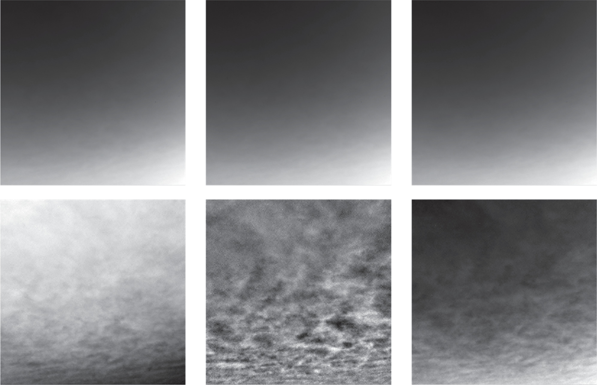
Figure 1. The three frames of the Sol 2633 pointing 5 movie before (top) and after (bottom) MFS. Cloud features that are not present in the raw frames are clear in the MFS frames.
Download figure:
Standard image High-resolution imageFollowing MFS, each perturbation movie is contrast stretched and manually examined to determine if clouds are present. If they are, a radiance map of frame 2 is created from the original images to determine the variation in spectral radiance between a region of assumed cloud and a region of assumed empty sky (Figure 2). We select points of high spectral radiance (presumed cloud) and low spectral radiance (presumed empty sky) and average over a circle of 5 pixel radius to determine the value of Iλ,VAR to be used in Equation (2). The value of Iλ,VAR should be taken as a lower limit due to uncertainty in whether the low-radiance region is truly empty sky or merely a thinner cloud. The selected location of the cloud within the frame is also used to calculate the scattering angle, θ.

Figure 2. A spectral radiance map of the second frame of the fifth pointing movie on Sol 2633 with a region of high spectral radiance (black dot) and low spectral radiance (red dot) indicated. The high-radiance region is assumed to be a cloud, while the low-radiance region is assumed to be empty sky. The color bar represents change in radiance relative to the mean value of the entire image.
Download figure:
Standard image High-resolution imageWhile it is difficult to account quantitatively for all errors associated with Equation (2), we can approximate the uncertainty from several sources. The MSL opacities used for this study have a mean uncertainty of around 20%, while the uncertainty on the Iλ,VAR term is likewise ∼20%. The contribution to uncertainty from τCOL is much lower, averaging ∼6% for the ACB seasons of MYs 34, 35, and 36. Taken together, these give an uncertainty of around 30% for our calculated phase function, when we use the MSL-derived cloud opacities.
Cooper et al. (2019) take an upper limit on MCS optical depths of 10%. Combined with the uncertainties on Iλ,VAR and τCOL, this gives an uncertainty of around 23% for the phase function. However, this does not take into account any uncertainties that may be associated with the fact that we are averaging the MCS opacities over 10° of Ls and five MYs.
2.3. Determining the Ice Crystal Habit from the Phase Function
In determining an ice crystal habit, and in comparing to previously derived water-ice cloud phase functions, the overall shape of the phase function is of more interest than its absolute magnitude. Typically, a phase function is normalized over scattering angles 0°–180° such that the area under the curve is equal to 4π (Hansen & Travis 1974). For instance, HG functions (discussed in more detail in Section 4.2) are normalized in such a way (Hapke 2012a). However, since more scattering from particles of comparable radius to Martian aerosols occurs in the forward scattering direction (scattering angles less than 40°), which the PFSS is not able to observe, it is not possible to determine what normalization values are appropriate for our derived phase function. As a result, our computed phase functions are normalized around the mean values of the phase functions to which we compare them.
3. Results
3.1. Temporal Distribution
Figure 3 shows the temporal distribution of the last three MYs of PFSS observations. The MY 34 data are described in detail in Cooper et al. (2019). In MY 35, there were a total of 26 PFSS observations, with 13 morning and 13 afternoon observations, spanning Ls = 55.0°–159.4°= (sols 2471 to 2691). In MY 36, there were a total of 30 PFSS observations, with 13 morning and 17 afternoon observations, spanning Ls = 43.7°–164.0° (sols 3115–3368). Of these, the two penultimate observations (sols 3353 and 3359) were excluded as they were taken during a regional dust storm, and it was not possible to determine if the features seen in the frames were water-ice clouds or dust features. Aside from the above exceptions, every observation contained at least one movie in which clouds could be positively identified, for a total of 167 movies in MY 35 and 191 movies in MY 36 showing cloud features.
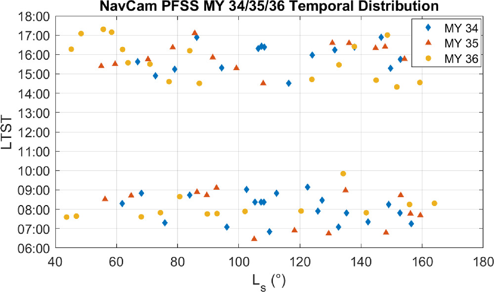
Figure 3. Temporal distributions of PFSS observations for the past three MYs. Observations are distributed between morning and afternoon with a ±2.5 hr keep-out around local noon.
Download figure:
Standard image High-resolution imageThe radiance points chosen from the movies and their corresponding calculated phase functions spanned scattering angles 46.4°–154.1° in MY 35 and 45.0°–139.9° in MY 36. These angular ranges are much narrower than that of MY 34, due mainly to our change in methodology that rejects scattering angles less than 45°.
3.2. Derived Phase Functions
We produced a mean phase-function curve for both MYs using the MCS cloud opacities, using a moving average with a window size of 15° of scattering angle. This window size remains fixed regardless of the number of points within the 15° bin. Figure 4 shows these curves with their 95% confidence intervals. Both phase functions have a greater magnitude at scattering angles >60°, which decreases with increasing scattering angle until the curve becomes approximately flat after about 100°.
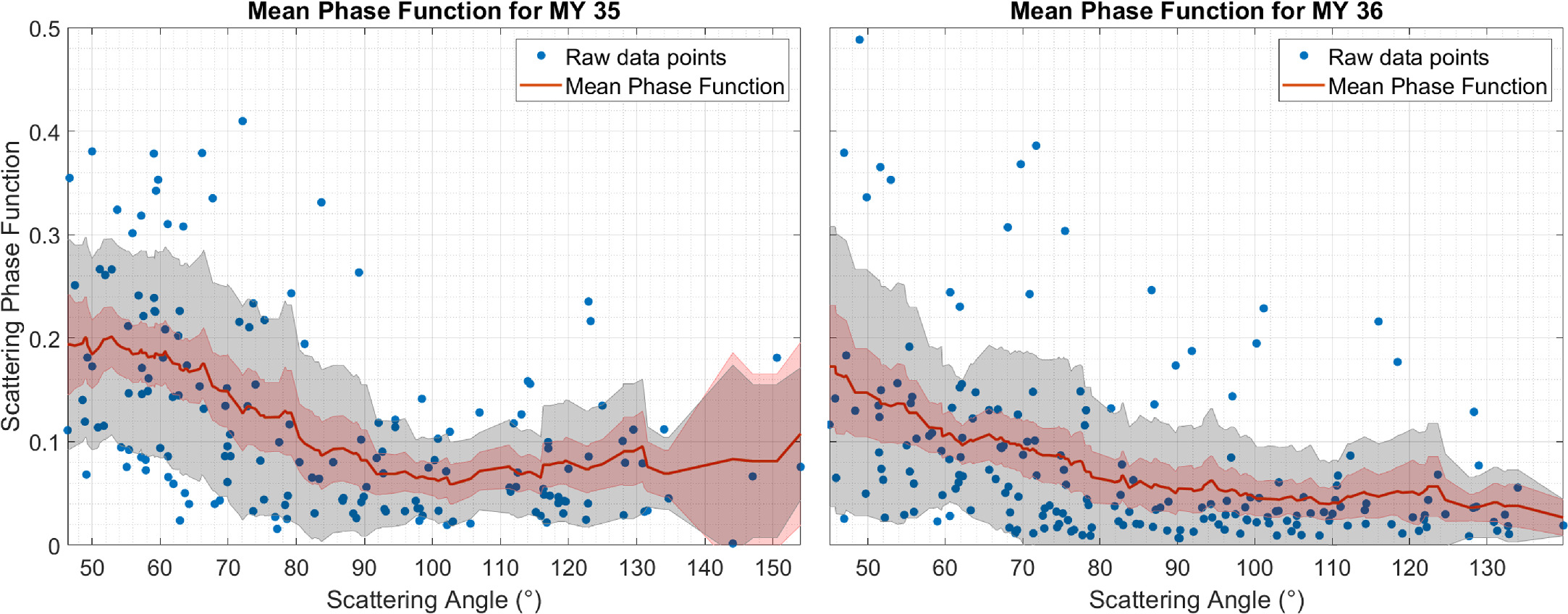
Figure 4. Mean curves of the derived phase-function data for MYs 35 and 36 displayed over their respective calculated raw data points. Red shaded error bars correspond to the 95% confidence interval, which is given by the expression  , while gray shaded error bars correspond to the standard deviation (σ). As with the mean curve, both were calculated by binning the data points with a window size of 15° of scattering angle. No normalization has been applied to magnitudes.
Download figure:
Standard image High-resolution imageWhen we compare our two derived curves to the Cooper et al. (2019) MY 34 curve (Figure 5), we see that all three phase functions have a similar shape, with small differences in normalized magnitude generally falling within their respective 95% confidence intervals.
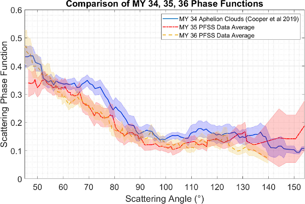
Figure 5. Comparison of MY 35 and 36 average phase functions with the Cooper et al. (2019) MY 34 phase function. MY 35 and 36 phase functions have been normalized around the average value of the MY 34 phase function. All three phase functions use MCS optical depth values. Shaded error bars show the 95% confidence interval.
Download figure:
Standard image High-resolution imageWe also derived mean phase-function curves using MSL water-ice tau values in the place of MCS column tau values. We rederived individual phase-function values and applied the same moving average to produce curves for all three MYs, as shown in Figure 6. As in the case of MY 35 above, we removed any outliers that had values greater than 3 standard deviations from the mean.
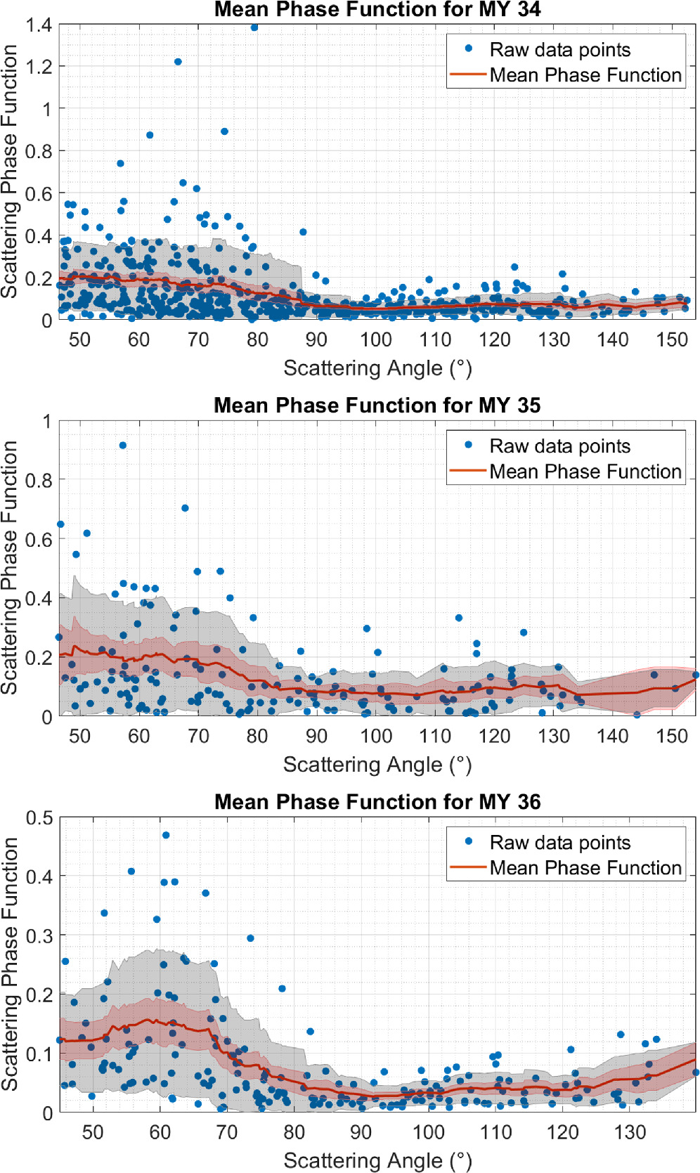
Figure 6. Mean phase functions for MY 34, 35, and 36, respectively, plotted with the raw calculated phase-function points. These phase-function values are calculated using MSL-derived tau values. The red shaded error bar corresponds to the 95% confidence interval, while the gray shaded error bar corresponds to the standard deviation. Outliers that are greater than 3 standard deviations from the mean have been removed. No normalization has been applied to magnitudes.
Download figure:
Standard image High-resolution imageAgain, all three phase functions agree closely with each other (Figure 7), and we see the increase in magnitude in the forward scattering direction and the flattening of the curve as scattering angle increases. The MY 36 phase function shows some increase in magnitude toward 140°; however, this is likely due to the relative paucity of data points at that range of scattering angles.

Figure 7. Comparison of MY 34, 35, and 36 mean phase functions, using phase function values calculated with MSL-derived tau values. The curves have been normalized to overlap in order to more easily compare their shapes. Shaded error bars show the 95% confidence interval.
Download figure:
Standard image High-resolution image3.3. Diurnal Variability
We were interested in exploring if there was any diurnal variability in ice crystal habit. Previous studies have shown the potential for diurnal variability at Gale Crater in both opacity (Kloos et al. 2018) and altitude (Campbell et al. 2020). These differences could be due to differences in temperature and formation mechanism, with morning clouds being a result of overnight clouds formation at lower temperatures and afternoon clouds formation due to enhanced convection (Tamppari et al. 2003). As a result, we wished to see if this would impact the cloud ice crystal habit. We derived mean morning and afternoon phase functions by taking morning and afternoon observations separately and applying the same moving average. Figure 8 shows a morning versus afternoon comparison for each MY using the MSL-derived tau phase function.
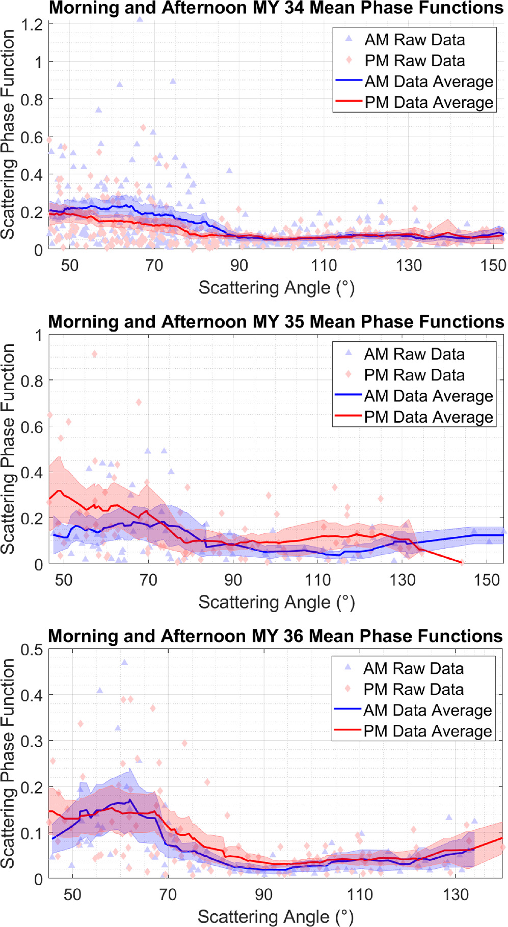
Figure 8. Comparisons of morning and afternoon mean phase functions plotted alongside their 95% confidence interval for each MY.
Download figure:
Standard image High-resolution imageFor all three MYs, the shapes of the mean curves are very similar to each other, which does not indicate a difference in phase function between the morning and afternoon clouds. It is not possible to definitively say whether the ice crystal habit is constant over the course of a sol, but such behavior would be consistent with our data.
4. Discussion
4.1. Challenges in Determining Tau in Phase Function Calculations
Like Cooper et al. (2019), we initially used MCS retrievals of column water-ice optical depth for the tau value of water-ice clouds to derive the phase function. However, our use of these MCS values does present some potential problems in our calculation of the phase function. Most obviously, the MCS tau values we use do not correspond one-to-one to the PFSS observations, and indeed the values we use are averaged over 10° of Ls and five MYs. As a result, we are not using tau values for the individual clouds we see in the PFSS observations but instead taking an average tau value for the apporximate time of year. Additionally, at low altitudes, the atmosphere becomes opaque and can become obscured by topography, which restricts the instrument's ability to detect water ice (Kleinböhl et al. 2009).
The use of tau values derived from MSL observations has several advantages over the use of MCS tau values. The MSL cloud observations from which the tau values are derived (zenith and suprahorizon movies, ZMs and SHMs) are often taken with the PFSS observation, and in most cases we were able to use tau values for clouds that were observed on the same sol and nearly at the same time as the PFSS observations. Only in a few cases were tau values taken from observations several sols (and thus only a few degrees of Ls ) before or after the PFSS. Additionally, the ZM and SHM also use the NavCams, meaning that the observations are in the same wavelength and have the same viewing geometry as the PFSS, namely looking at the clouds from below. This means in most cases we can be sure that we are observing the same clouds and deriving a tau value that is representative of those specific clouds.
That being said, neither approach is without weakness. The MSL-derived tau values are calculated using an assumed phase function, the weaknesses of which are discussed in Hayes et al. (2023). However, given the advantages in seeing either the same clouds, or at least temporally nearby clouds, we have made the choice to continue using the phase-function values calculated with MSL-derived tau values.
4.2. Constraining Ice Crystal Habit
Cooper et al. (2019) attempted to constrain a dominant ice crystal habit through comparing their derived phase function with modeled phase functions of seven randomly oriented water-ice crystals (Figure 7 in Cooper et al. 2019). They found that the phase function did not fit any one of the curves for the ice crystal geometries particularly well. As our derived phase functions are very similar in shape to that of Cooper et al. (2019; Figure 9), we may expect to see similar results. However, it is likely that this method of comparison is not optimal for Martian water-ice clouds. The water-ice crystal data set used by Cooper et al. (2019) assumed very large water-ice particle sizes on the order of tens of microns (Yang & Liou 1996; Yang et al. 2003), while Martian water-ice crystals tend to be much smaller (Clancy et al. 2003). In addition, the formation of Martian water-ice clouds, with much less water vapor aggregating on a much greater number density of dust particles that serve as cloud condensation nuclei, may create some unusual or irregular geometries for which there is no good terrestrial analog. While the halo seen by Perseverance does strongly imply a crystal size and shape (Lemmon et al. 2022), it is a single occurrence that has not been seen in over five MYs of observations at Gale Crater.
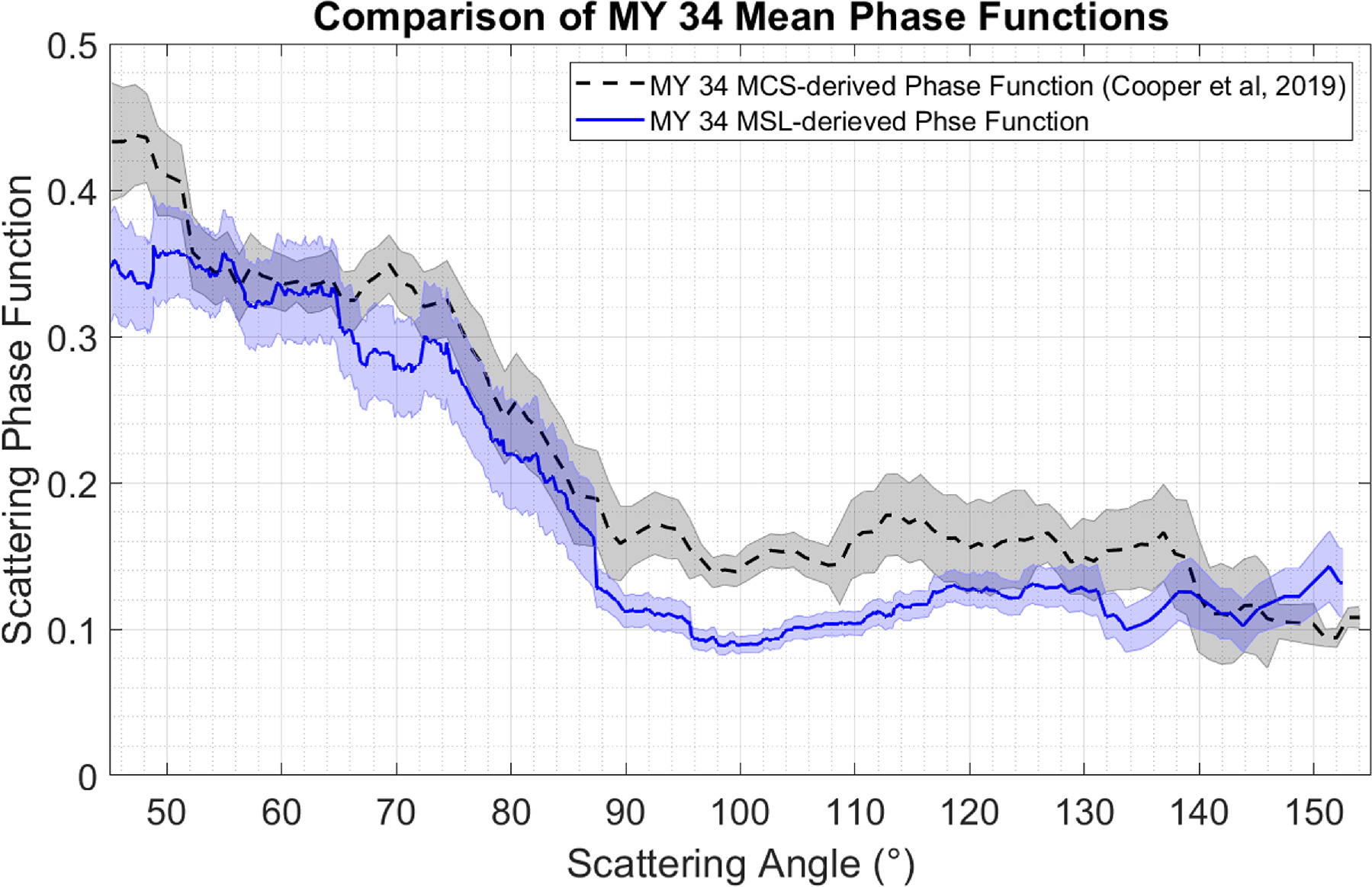
Figure 9. Comparison of MY 34 phase functions derived by Cooper et al. (2019) using MCS opacities (black dashed line) and derived using MSL-derived opacities (blue solid line) plotted with 95% confidence intervals. The MSL-derived mean phase function has been normalized by the mean value of that of Cooper et al. (2019).
Download figure:
Standard image High-resolution imageWe instead use a different method of determining likely ice crystal habit, by fitting a two-term HG function to our calculated phase-function values. HG functions can be used to approximate single scattering phase functions, with a two-term HG function representing bidirectional scattering (Hapke 2012a). HG functions have a history of use in planetary applications though mostly for modeling the phase functions of dust and regolith (Hapke 2012b). Despite this, we believe that it is a good fit for our application as it is, at its core, used to represent single scattering phase functions, which we have derived for the PFSS results. Additionally, it allows us to easily compare our results to various airborne dust particles, which have been modeled in similar ways.
We use a two-term HG function similar to that used by Moores et al. (2015), who examined dust cover on the Phoenix Lander telltale mirror:
where c is the backscatter fraction and b is the asymmetry parameter. Small values of b give low, wide forward- and backscattering lobes, while larger values give higher, narrower lobes. Higher values of c indicate smaller amounts of forward scattering (Hapke 2012b).
Different authors have defined c in different ways. Hapke (2012a) uses a value of c, which gives the two-term HG function as
where g is the phase angle. Thus, our value of c can be related to the Hapke (2012a) value (cH) by

Hapke (2012b) created a plot of b versus c values for 495 regolith and dust particles, which lie within a region of physically allowable values resembling a hockey-stick shape (Figure 2 of Hapke 2012b). The centroid of this region is given by a "hockey-stick relation" (Equation (8) of Hapke 2012b).
We fit the HG function (Equation (3)) to the full range of data for each MY. Figure 10 shows these b and c values, with error bars representing the 95% confidence bounds in b and c. While the asymmetry parameter, b, appears fairly well constrained especially compared to c, this is only the case within the bounds of our data, between scattering angles of 45° and 155°. These limitations on our data set mean that we are not seeing the areas where we would expect to see most scattered light, and therefore the fit HG functions for each MY are only our best guesses with the data available.

Figure 10. b and c values for fitted HG functions for MYs 34–36 plotted alongside the hockey-stick relation for two-term HG functions determined by Hapke (2012b). Error bars show the 95% confidence bounds on b and c.
Download figure:
Standard image High-resolution imageOur b and c values fall near the hockey-stick curve and within the allowable bounds established by Hapke (2012b; Equation (6) in that work). In addition, our values fall near those reported by Souchon et al. (2011), which looked at volcanic samples, particularly irregular, rough, opaque glass and round, smooth, translucent glasses. While the cloud particles we observe are not necessarily exactly these materials, we may see similar irregular, rough shapes. This could also indicate we are seeing igneous dust particles with ice accreted onto it.
As a point of comparison, we fit the same HG function to the phase functions of six modeled water-ice crystals with particle sizes around 3 μm (Bi & Yang 2014). These are different phase functions than were used by Cooper et al. (2019), which had much larger particle sizes. The ones we use are on the order of likely Martian water-ice crystal sizes (Clancy et al. 2003). We plot the determined b and c values alongside those we found for the PFSS results.
We also compare our results with those for Martian dust particles. HG functions have been used to fit Martian dust like that seen at the Spirit rover site (Johnson et al. 2006), the Phoenix lander site (Moores et al. 2015), and, most relevantly to this study, Gale Crater (Chen-Chen et al. 2019). Johnson et al. (2006) found an HG function for the Martian simulant HWMK919 at various wavelengths. We use their results at 750 nm, which falls within the bandpass of the MSL Navcams. The Chen-Chen et al. (2019) results also use observations from the Navcams but use a three-term HG function. We fit our two-term expression to their three-term curve in order to extract b and c values. The Surface Stereo Imager on board Phoenix used in the Moores et al. (2015) study is centered at 450 nm, outside the bandpass of the Navcams. We also include the b and c values for a theoretical perfect, clear sphere as determined by McGuire (1995) for comparison.
We see (Figure 11) that our b and c values do fall relatively near several of the other phase functions, especially the Navcam-observed dust. We also note that our phase function does not fit particularly well to that of the theoretical sphere. This is of note given that many climate models assume spherical water-ice crystal geometry. The closest of the modeled water-ice crystals to our own phase function is droxtals, which is of interest as that geometry is used in the single scattering phase function of Wolff et al. (2019).

Figure 11. b and c values for our derived phase functions compared with fitted HG curves for six modeled water-ice crystal geometries (Bi & Yang 2014); Martian dust observed by MSL (Chen-Chen et al. 2019) and Phoenix (Moores et al. 2015) and a simulant similar to dust observed by Mars Exploration Rover Spirit (Johnson et al. 2006); and a theoretical smooth, transparent sphere (McGuire 1995). All values are displayed alongside the hockey-stick relation for two-term HG functions determined by Hapke (2012b). Error bars on our derived phase function are the 95% confidence bounds on our b and c values.
Download figure:
Standard image High-resolution image
Due to our narrow range of scattering angles, there is some inherent uncertainty associated with our fit HG functions as we do not see either the forward- or backscattering lobes. Additionally, the method of fitting an HG function has been used primarily in planetary applications to look at the phase function of regoliths and dusts, and as such, there are not many good points of comparison for water-ice particles.
5. Conclusions
In this work, we extended the PFSS campaign of Cooper et al. (2019) through two additional MYs and analyzed 3 yr of observations with a modified procedure for calculating a phase function using MSL-derived values of cloud opacity. While these values give us similarly shaped phase functions to those derived using MCS tau values, they are closer temporally to the PFSS observations, meaning we can use optical depth values of the actual clouds observed in the PFSS rather than an average value. The mean curves for all 3 yr have very similar shapes, as might be expected given the high repeatability of the ACB. Likewise, we do not see any difference in the mean curve of morning or afternoon clouds, suggesting that the ice-particle phase function remains relatively consistent throughout the day.
In an attempt to determine what that ice crystal habit may be, we fit a two-term HG function in order to help constrain the dominant ice crystal geometry of the observed water-ice clouds. In comparing our HG functions to fit HG functions of Martian dust and several modeled water-ice crystals, we see some overlap in the b parameter, especially with dust at Gale Crater and droxtal-shaped water-ice crystals. We also see agreement in b and c parameters with rough, irregular volcanic glasses, which lends support to the assumption that the observed water-ice crystals have some irregular geometry.
Acknowledgments
This work was partly funded by a Natural Sciences and Engineering Research Council of Canada (NSERC) Technologies for Exo-Planetary Science (TEPS) Collaborative Research and Training Experience (CREATE) grant #482699 and the Canadian Space Agency's MSL Participating Scientist Program.
The authors thank the Mars Science Laboratory science and operations teams.