Abstract
In this work, we consider the inverse scattering problem of determining an unknown refractive index from the far-field measurements using the nonparametric Bayesian approach. We use a collection of large 'samples', which are noisy discrete measurements taking from the scattering amplitude. We will study the frequentist property of the posterior distribution as the sample size tends to infinity. Our aim is to establish the consistency of the posterior distribution with an explicit contraction rate in terms of the sample size. We will consider two different priors on the space of parameters. The proof relies on the stability estimates of the forward and inverse problems. Due to the ill-posedness of the inverse scattering problem, the contraction rate is of a logarithmic type. We also show that such contraction rate is optimal in the statistical minimax sense.
Export citation and abstract BibTeX RIS

Original content from this work may be used under the terms of the Creative Commons Attribution 4.0 license. Any further distribution of this work must maintain attribution to the author(s) and the title of the work, journal citation and DOI.
1. Introduction
In this work, we study the Bayes method for solving the inverse medium scattering problem. Our aim is to prove the consistency property of the posterior distribution. Let the refractive index  and
and  be a compactly supported function in
  with
with  , where D is an open bounded smooth domain, and having suitable regularity, which will be specified later. Let
  satisfy

and

Assume that  is the plane incident field, i.e.
  with
with  , where
  . Then the scattered field
  satisfies

where  , see for example, [Ser17, p 232]. The inverse scattering problem is to determine the medium perturbation
  from the knowledge of the scattering amplitude
 for all
  at one fixed energy κ2.
It was known that the scattering amplitude  uniquely determines the near-field data of (1.1a
) on
uniquely determines the near-field data of (1.1a
) on  , which in turn, determines the Dirichlet-to-Neumann map of (1.1a
) provided κ2 is not an Dirichlet eigenvalue of
, which in turn, determines the Dirichlet-to-Neumann map of (1.1a
) provided κ2 is not an Dirichlet eigenvalue of  on D, for example, see [Nac88]. Combining this fact and the uniqueness results proved in [SU87], one can show that the scattering amplitude
  for all
  uniquely determines n, at least when n is essentially bounded. For the stability, a log-type estimate was derived in [HH01].
In this paper, we would like to apply the Bayes approach to the inverse scattering problem. The study of this inverse method is motivated by the practical consideration. In practice, it is impossible to obtain the full knowledge of the scattering amplitude. Instead, the following experiment is more realistic. We first randomly choose an incident direction and send out the corresponding incident field towards the probe region. Then we measure the scattering amplitude at another randomly chosen direction. The experiment can be repeated as many times as we wish. The goal now is to make an inference of the refractive index based on such observation data. To describe the method more precisely, we first introduce the measurement model. Let µ be the uniform distribution on  , i.e.
  , where
  is the product measure on
  , that is,
  . We also write
  and hence
  . Consider the iid random variables
  ,
,  with
with  . In other words,
  is a sequence of independent samples of µ on
  . Denote

where  is a realization of Xi
. The observation of the scattering amplitude
is a realization of Xi
. The observation of the scattering amplitude  is polluted by the measurement noise which is assumed to be a Gaussian random variable. Since
  is a complex-valued function, we treat it as a
  -valued function. For convenience, we slightly abuse the notation by writing
Consequently, the statistical model of the scattering problem is given as

where σ > 0 is the noise level, I2 is the  unit matrix. We also assume that
  and
and  are independent.
The theme of this paper is to consider the inference of n from the observational data  with
with  by the Bayes method. In particular, we are interested in the asymptotic behavior of the posterior distribution induced from a large class of Gaussian process priors on n as
  . The aim is to establish the statistical consistency theory of recovering n in (1.1c
) with an explicit convergence rate as the number of measurements N increases, i.e. the contraction rate of the posterior distribution to the 'ground truth' n0 when the observation data is indeed generated by n0. Gaussian process priors are often used in applications in which efficient numerical simulations can be carried out based on modern MCMC algorithms such as the pCN (preconditioned Crank–Nicholson) method [CRSW13].
. The aim is to establish the statistical consistency theory of recovering n in (1.1c
) with an explicit convergence rate as the number of measurements N increases, i.e. the contraction rate of the posterior distribution to the 'ground truth' n0 when the observation data is indeed generated by n0. Gaussian process priors are often used in applications in which efficient numerical simulations can be carried out based on modern MCMC algorithms such as the pCN (preconditioned Crank–Nicholson) method [CRSW13].
The study of inverse problems in the Bayesian inversion framework has recently attracted much attention since Stuart's seminal article [Stu10] (also see [DS17]). The setting of the problem considered in this paper is closely related to the ones studied in [GN20, Kek22]. In [GN20], Gaussian process priors were used in the Bayesian approach to study the recovery of the diffusion coefficient in the elliptic equation by measuring the solution at randomly chosen interior points with uniform distribution. It was shown that the posterior distribution concentrates around the true parameter at a rate N−λ
for some λ > 0 as  , where N is the number of measurements (or sample size). Previously, (frequentist) consistency of Bayesian inversion in the elliptic PDE considered in [GN20] was derived in [Vol13]. However, the contraction rates obtained in [Vol13] were only implicitly given. Based on the method in [GN20], similar results were proved in [Kek22] for the parabolic equation where the aim is to recover the absorption coefficient by the interior measurements of the solution. For further results on the Bayesian inverse problems in the non-linear settings, we refer the reader to other interesting papers [Abr19, NS17, NS19, MNP21, Nic20, NP21, NW20]. On the other hand, for linear inverse problems, the statistical guarantees of nonparametric Bayesian methods with Gaussian priors have been extensively studied and well understood, see for example [ALS13, KLS16, KvdVvZ11, MNP19, Ray13] and references therein.
The ideas used in proving the consistency of the Bayesian inversion for the inverse scattering problem studied here are similar to those used in [GN20, Kek22] in which main ideas are from [MNP21]. Unlike the polynomial contraction rates derived in [GN20, Kek22], the posterior distribution  of
of  contracts at the true refractive index n0 as
  with a logarithmic rate. The logarithmic rate is due to the ill-posedness of the inverse scattering medium problem by the knowledge of the scattering amplitude at one fixed energy, see [HH01].
This paper is organized as follows. In section 2, we describe the statistical model arising from the scattering problem. We state main consistency theorems with contraction rates assuming re-scaled Gaussian processes priors and re-scaled Gaussian sieve priors. The proofs of theorems are given in section 3. In appendix
2. The statistical inverse scattering problem
2.1. Some function spaces and notations
Throughout this paper, we shall use the symbol  and
and  for inequalities holding up to a universal constant. For two real sequences
  and
and  , we say that
  if both
  and
and  for all sufficiently large N. For a sequence of random variables ZN
and a real sequence
for all sufficiently large N. For a sequence of random variables ZN
and a real sequence  , we write
  if for all ε > 0 there exists
  such that for all N large enough,
  . Denote
  the law of a random variable Z. Let
  with
with  denote the Hölder space of order t with compact supports in the bounded smooth domain
  .
.
Let D be a bounded smooth domain in  , let
, let  be an integer and we consider the Hilbert space
For non-integer s,  is defined in terms of the interpolation, see [LM72]. It is known that the restriction operator to D is a continuous linear map of
  to
to  [LM72, (8.6)]. The space
  is the completion of
  with respect to
  . Also, for
  with
with  , the zero extension of
  (extension of f by 0 outside of D) is a continuous map
  [LM72, theorem 11.4]. Let
  be a compact subset, define
  . In fact, we have

see [McL00, theorems 3.29 and 3.33].
We now define the space of parameters. For  and
and  , let
, let

where the traces are defined in the sense of [LM72, theorem 8.3]. For each  we extend
  in
in  , still denoted by n. Then it is clear that
  . Note that for
  , we only put the restriction on the size of n, but not on the
  -norm of n. As in [NvdGW20, GN20, AN19, Kek22], we will consider a re-parametrization of
  . We consider the link function Φ satisfying
- (i)
 , , for all z;
 - (ii)for any
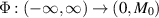


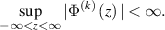
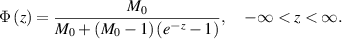
One example to satisfy (i) and (ii) is the logistic function
As pointed out in [NvdGW20, section 3], by utilizing a characterization of the space  (see e.g. [LM72, theorem 11.5]), one can show that the parameter space can be realized as

We end this subsection by emphasizing that our link function is different to those in [NvdGW20, GN20, AN19, Kek22], see (i).
2.2. An abstract statistical model
For each forward map
 , we define the reparametrized forward map by

and consider the following random design regression model

Assume that  satisfies

and for each  one has

for some constant  and
and  .
.
Remark 2.1. We implicitly assume that taking pointwise value of  on
on  is legitimate. For instance, in the inverse scattering problem here,
  (corresponding to the scattering amplitude
  ) is, in fact, analytic on
  .
.
The statistical model (2.2b
) with conditions (2.2c
) and (2.2d
) falls into the general framework described in [GN20]. We want to remark that the uniform boundedness of the forward map  (condition (2.2c
)) in [GN20, NvdGW20] (elliptic boundary value problem) or in [Kek22] (parabolic initial-boundary value problem) is ensured by the positivity assumption of the coefficient and the bound S1 is determined by the fixed boundary value or the fixed initial and boundary values. Due to these facts, the ranges of the link functions used in [GN20, NvdGW20] and [Kek22] do not required to have finite upper bounds. In the scattering problem, the boundedness requirement of the forward map (2.2c
) cannot be guaranteed by the sign restriction of the potential. In this case, we choose a link with finite range (like Φ given above) to ensure (2.2c
).
(condition (2.2c
)) in [GN20, NvdGW20] (elliptic boundary value problem) or in [Kek22] (parabolic initial-boundary value problem) is ensured by the positivity assumption of the coefficient and the bound S1 is determined by the fixed boundary value or the fixed initial and boundary values. Due to these facts, the ranges of the link functions used in [GN20, NvdGW20] and [Kek22] do not required to have finite upper bounds. In the scattering problem, the boundedness requirement of the forward map (2.2c
) cannot be guaranteed by the sign restriction of the potential. In this case, we choose a link with finite range (like Φ given above) to ensure (2.2c
).
Remark 2.2. In view of (1.2) and (2.1), one notes that the statistical model (1.3) fits into the framework of (2.2b
). For the inverse scattering problem studied here, if the forward map G(n) is defined by the far-field pattern (1.2) with refractive index  with
with  , from (A.9) we see that (2.2c
) satisfies with
, from (A.9) we see that (2.2c
) satisfies with  . From (A.14) we have

where  . By using (ii) and [NvdGW20, lemma 29], we have

and

therefore we see that (2.2d
) satisfies with  with t = 1.
Observe that the random vectors  are iid with laws
  . It turns out the Radon–Nikodym derivative of
  is given by

By slightly abusing the notation, now we define  the joint law of the random vectors
  . Moreover,
  ,
,  denote the expectation operators in terms of the laws
  , respectively.
In the Bayesian approach, let Π be a Borel probability measure on the parameter space  supported in the Banach space C(D). From the continuity property of
  , the posterior distribution
  of
of  is given by
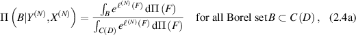
where the log-likelihood function is written as

Finally, we end this subsection by referring to the monograph [Nic23] for a nice introduction on the above preliminaries.
2.3. Statistical convergence rates
In this work we would like to show that the posterior distribution arising from certain priors concentrates near sufficiently regular ground truth  , and derive a bound on the rate of contraction, assuming that the observation data
  are generated through the model (2.2a
)–(2.2d
) of law
are generated through the model (2.2a
)–(2.2d
) of law  .
.
2.3.1. Rescaled Gaussian priors.
We now describe explicitly Gaussian priors introduced in [GN20] (also see [Kek22]).
Assumption 2.3. Let  ,
,  , and
, and  be a Hilbert space continuously embedded into
  , and let
  be a centered Gaussian Borel probability measure on the Banach space
  that is supported on a separable measurable linear subspace of
  . Assume that the reproducing kernel Hilbert space (RKHS) of
  equals to
  .
.
Here, we refer to [GN21, definition 2.6.4] for the definition of the RKHS, and we refer to [GN20, example 25] for an example satisfies assumption 2.3. For each s given in assumption 2.3, let  be given in assumption 2.3 and
  , we consider the rescaled prior

Again,  defines a centered Gaussian prior on C(D) and its RKHS
  is still
  but with the norm

for all  . We now introduce the main device in our proof, concerning the posterior contraction with an explicit rate around F0, whose proof can be found in [GN20, theorem 14].
Theorem 2.4. Let  satisfies assumption 2.3 with integer s, let
 ![$\Pi_{N}\equiv\Pi_{N}[s]$](https://content.cld.iop.org/journals/0266-5611/40/5/055001/revision2/ipad3089ieqn136.gif) be the rescaled prior given in (2.5), let
be the rescaled prior given in (2.5), let  be the posterior distribution given in (2.4a
) with
be the posterior distribution given in (2.4a
) with  . Assume that
  and the observation
  to be generated through model (2.2b
)–(2.2d
) of law
to be generated through model (2.2b
)–(2.2d
) of law  . If we denote
  , then for any K > 0, there exists a large L > 0, depending on
  , such that
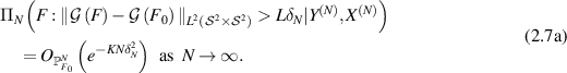
In addition, there exists a large  , depending on
  , such that

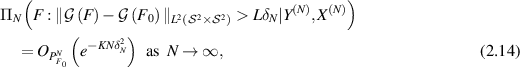
We now apply theorem 2.4 to the inverse scattering problem considered here. Relying on the contraction rate (2.7a
) and the regularization property (2.7b
) and taking account of the stability estimate of G−1 (see theorem A.1), we can show that the posterior distribution arising from the statistical inverse scattering model (1.3) contracts around n0 in the  -risk using ideas from [MNP21]. In light of the link function, we define the push-forward posterior on the refractive index n by

By the push-forward map, we can rewrite (2.7a
) and (2.7b
) in terms of n. That is, we have that for  that
that

and

where the second estimate can be derived from the estimates proved in [NvdGW20, lemma 29] (see also [GN20, (27)]). Here L depends on  and Lʹ depends on
  .
.
Theorem 2.5. Let  and
and  be integers, and fix a real parameter
  . We further assume that
  is any constant satisfying
  . Let
. Let  ,
,  and
and  be given in theorem 2.4. The ground truth refractive index is
  . Then for any K > 0, there exists a constant
  such that

as  .
.
It is clear that we can replace  by
by  in (2.9). Unlike the polynomial rate proved in [GN20, theorem 5], we obtain a logarithmic contraction rate in (2.9), which is due to a log-type stability estimate of G−1. To obtain an estimator of the unknown coefficient n, in view of the link function Φ, it is often convenient to derive an estimator of F. The posterior mean
 ![$\bar F_N : = \mathbb{E}^{\Pi}[F|Y^{(N)},X^{(N)}]$](https://content.cld.iop.org/journals/0266-5611/40/5/055001/revision2/ipad3089ieqn162.gif) of
of  , which can be approximated numerically by an MCMC algorithm, is the most natural choice of estimator. In light of theorem 2.5, we can also prove a contraction rate for the convergence
  to F0.
Theorem 2.6. Assume that the hypotheses of theorem 2.5 hold. Then, there exists a  such that

Corollary 2.7. Assume that the hypotheses of theorem 2.5 hold. Then there exists a sufficiently large  such that

The logarithmic contraction rates obtained in theorems 2.5, 2.6, and corollary 2.7 inherit from the log-type estimate of the inverse scattering problem. Nonetheless, in the next theorem, we will show that this contraction rate for the estimator  is optimal is the statistical minimax sense, at least up to the exponent of
  . We first define a parameter space. Let
  be an integer, β > 0, and define

Theorem 2.8. For integer  , there exists
  such that for any
  and
and  , we have

for all N large enough, where the infimum is taken over all measurable functions  of the data
  .
.
2.3.2. High-dimensional Gaussian sieve priors.
From computational perspective, it is useful to consider sieve priors that are finite-dimensional approximations of the function space supporting the prior. Here we will use a randomly truncated Karhunen–Loéve type expansion in terms of Daubechies wavelets considered in [GN20, appendix B] or [GN21, chapter 4]. Let  be the (3-dimensional) compactly supported Daubechies wavelets, which forms an orthonormal basis of
  . Let
. Let  be a compact subset in D and let
  . Let
. Let  be another compact subset in D such that
  , and let
  be a cut-off function with χ = 1 on
  . Let
. Let  and consider the prior

where  is the truncation level. In fact
  defines a centered Gaussian prior that is supported on the finite-dimensional space

with RKHS norm satisfying [GN20, (B2)]. As above, we consider the 're-scaled' prior  defined in (2.5) with
  .
.
In analogy to theorem 2.4, we will derive a contraction rate for the statistical model (2.2b
) with the prior  defined above. As in theorem 2.4, we obtain the same contraction rate in the L2-prediction risk of the regression function.
Theorem 2.9. Let  ,
,  be integers, and
 ![$\Pi_N\equiv \Pi_{N}[s]$](https://content.cld.iop.org/journals/0266-5611/40/5/055001/revision2/ipad3089ieqn192.gif) be the 're-scaled' prior defined in (2.5) with priors
be the 're-scaled' prior defined in (2.5) with priors ![$F^{^{\prime}}\sim\Pi^{^{\prime}}_{J_{N}} \equiv \Pi^{^{\prime}}_{J_{N}}[s]$](https://content.cld.iop.org/journals/0266-5611/40/5/055001/revision2/ipad3089ieqn193.gif) where
where  . Denote
  the posterior distribution arising from the noisy discrete measurements
  of (2.2b
). Let
of (2.2b
). Let  and
and  . Then for any K > 0, there exists a large L > 0, depending on
  , such that
and for sufficiently large  , depending on
  , we have

The proof of theorem 2.9 only requires minor modification from the proof of theorem 2.4, and all necessary modifications are listed in [GN20, section 3.2]. Therefore we omit the details. Having established theorem 2.9, similar to [GN20, proposition 7], theorems 2.5 and 2.6 can be directly extended to the case of Gaussian sieve priors.
Remark 2.10. As in [GN20], it is likely to extend the results for the Gaussian sieve priors with deterministic truncation level to randomly truncated ones, where the truncation level J itself is an appropriate random number. However, due to the log-type stability estimate of the inverse scattering problem, such extension is highly nontrivial. We will discuss the Bayes method with randomly truncated sieve priors for the inverse scattering problem in another paper.
3. Proofs of theorems
The main theme of this section is to prove theorem 2.5, 2.6 and 2.8.
Proof of theorem 2.5. For each M > 0 satisfies  , one has the stability estimate of G−1 in theorem A.1:

where  and
and  .
.
If  for some
  , since t is an integer, then
  with
with  . We now set the constant
  . In view of (2.8a
), (2.8b
), and (3.1), for any K > 0, there exists large constants
. In view of (2.8a
), (2.8b
), and (3.1), for any K > 0, there exists large constants  and Lʹ (Lʹ is determined by L and Mʹ) such that
which conclude our result. □
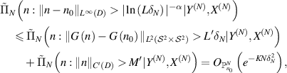
Having proved theorem 2.5, we then establish theorem 2.6 using the contraction rate in theorem 2.5 and the link function Φ.
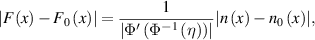
Proof of theorem 2.6. We proof the theorem by modifying some ideas in [GN20, theorem 6]. By the Jensen's inequality, it suffices to prove that there exists a large  such that

For a large M > 0 to be chosen later, we write
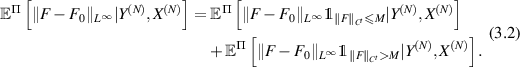
Part I: Estimating ![$\mathbb{E}^\Pi[\|F-F_0\|_{L^\infty}{\unicode{x1D7D9}}_{\|F\|_{C^t}\gt M}|Y^{(N)},X^{(N)}]$](https://content.cld.iop.org/journals/0266-5611/40/5/055001/revision2/ipad3089ieqn212.gif) . By using Cauchy-Schwartz inequality, it is easy to see that
. By using Cauchy-Schwartz inequality, it is easy to see that
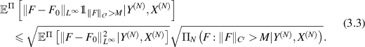
Let B > 0 be a constant to be determined later. By using (2.7b
), one can choose a sufficiently large  such that
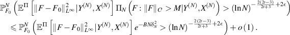
We now define  by
by

By using [GN20, lemmas 16 and 23], we have

Let  and set the event

By [GN21, lemma 7.3.2], we can show that

By using the properties (3.6) of  , we obtain
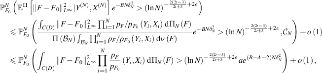
which is bounded from above, using Markov's inequality and Fubini's theorem, by
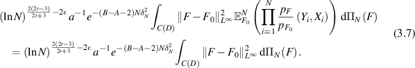
By using Fernique's theorem (see e.g. [GN21, exercises 2.1.1, 2.1.2 and 2.1.5]) one has  . Taking
  , from (3.7) we conclude

Part II: Estimating ![$\mathbb{E}^\Pi[\|F-F_0\|_{L^\infty}{\unicode{x1D7D9}}_{\|F\|_{C^t} \unicode{x2A7D} M}|Y^{(N)},X^{(N)}]$](https://content.cld.iop.org/journals/0266-5611/40/5/055001/revision2/ipad3089ieqn219.gif) . The above discussions still valid if we replace M by a (possibly larger)
. The above discussions still valid if we replace M by a (possibly larger)  with
with  . Since
  and
and  , by (i), mean value theorem and inverse function theorems, there exists η lying between
  and n(x) such that
for all  . Since
 ![$F,F_{0} \in \left[\Phi(-M),\Phi(M)\right]$](https://content.cld.iop.org/journals/0266-5611/40/5/055001/revision2/ipad3089ieqn226.gif) , by (i) we reach
, by (i) we reach

Therefore we see that

and

Let C > 0 be a constant to be determined later. From (3.9), we see that
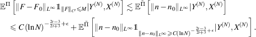
We can modify the arguments as in Part I above by replacing the event  (resp. (2.7b
)) by the event
(resp. (2.7b
)) by the event  (resp. (2.9)) with
  given in theorem 2.5 to show that

Finally, putting together (3.2), (3.8), and (3.10) yields theorem 2.6 with  . □
. □
Next, we prove the optimality of contraction rate in corollary 2.7 in the minimax sense.
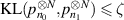
Proof of theorem 2.8. We apply the method in the proof of the lower bound [AN19, theorem 2] to our case here. The idea is to find  (both are allowed to depend on N) such that, for some small ζ sufficiently small,
- (a).
- (b),

where  is the Radon Nikodym derivative of the joint law
  and the Kullback–Leibler divergence
  is defined by

By independence, we note that
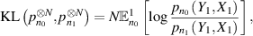
and [GN20, lemma 23] implies

then using the standard arguments as in [GN21, section 6.3.1] (see also [Tsy09, chapter 2]), we conclude the theorem.
For the sake of completeness, here we present the details. From condition (a), we see that  yields a test of

It follows from a general reduction principle that

where the second infimum is over all tests ψ of (3.13). Similar to the proof of [GN21, theorem 6.3.2], we introduce the event
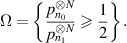
Note that

Let  , then
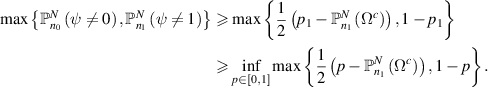
It is clear that the infimum above is attained when  and has the value
  . Hence,

Next, let us estimate
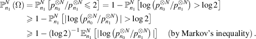
Using the second Pinsker inequality [GN21, proposition 6.1.7b] and condition (b), we have
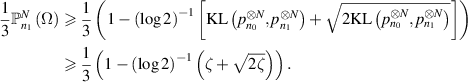
We now choose ζ sufficiently small such that the last term above is bounded below by  . Then the estimate (2.12) follows in view of (3.14).
The remaining task is to find  satisfying conditions (a) and (b). For
  , setting
  in theorem B.1, there exist
  satisfying
  and
and

To verify condition (b), we use (3.12) to conclude that
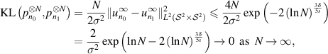
since  . Therefore, we can make ζ as small as we wish by taking N sufficiently large. □
Data availability statement
No new data were created or analysed in this study.
Appendix A: Inverse scattering problem
In what follows, assume that

We first discuss the existence and uniqueness of the scattered field  . It is known that
  satisfies the following boundary value problem [CCH23, (1.51)–(1.52)]:

where BR
is a ball of radius R such that  . Here
  is the Dirichlet-to-Neumann map, defined for
  by
by  , where ug
is the solution of the Helmholtz equation satisfying the Sommerfeld radiation condition in
, where ug
is the solution of the Helmholtz equation satisfying the Sommerfeld radiation condition in  and the Dirichlet condition
  on
on  . It has been shown that

where  denotes the duality pairing between
  and
and  , see, for example, [CCH23, definition 1.36 and (1.50)].
To proceed further, let us replace the right-hand side of the first equation in (A.2) by a general source term f with  , i.e.

In view of the integration by parts, (A.4) is equivalent to the following variational formulation: find  such that for all
  ,
,

where

and
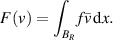
We can see that

In other words,  is strictly coercive. Combining the Riesz representation theorem and the Lax–Milgram theorem, there exists an invertible operator
  , where
  is the dual space of
  , such that

Similarly, define the bounded linear operator  by
by  . It is not difficult to see that
  is compact. Consequently,
  is a Fredholm operator. By the Fredholm alternative,
  is bounded invertible provided the kernel of
  is trivial, which follows the uniqueness of the scattered solution (by the combination of the Rellich lemma and the unique continuation property). Furthermore, we have the following estimate:

where  . Let
. Let  and
and  , then (A.5) implies

uniformly in  . We now choose
  such that
  . By the interior estimate [GT01, theorem 8.8], we further have

which, by the Sobolev imbedding theorem, implies

The scattering amplitude  can be expressed explicitly by
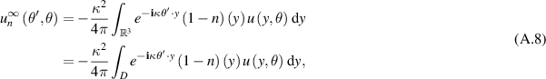
where  is the total field with
  , see [CCH23, (1.22)] or [CK19, (8.28)] or [Ser17, p 232]. From (A.7) and (A.8), we have

with  . Since

applying the interior estimate and the Sobolev imbedding theorem again, we have that

with  .
.
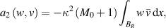
Next, assume that  satisfy (A.1). For each open set Ω in Euclidean space, we observe that
Let  and
and  , then combining (A.5), (A.7), (A.10) and (A.11), yields

uniformly in θ and  . Then it yields from (A.8) that
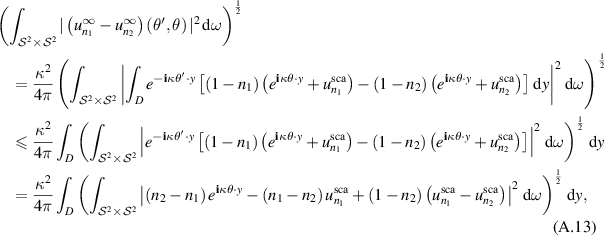
where the inequality above is due to the integral form of Minkowski's inequality. Plugging (A.6), (A.10) and (A.12) into (A.13) gives

where  .
.
Next, we recall the following stability estimate for the determination of the potential from the scattering amplitude.
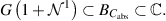
Theorem A.1
(HH01, theorem 1.2). Let  , M > 0, and
  be given constants. Assume that
  satisfying
  and
and  ,
,  . Then

where  and
and
Remark A.2 Here the constant M may be different from M0 given above.
Appendix B: Optimality of the stability estimate
The purpose of this section is to show that the logarithmic estimate obtained in theorem A.1 is optimal by deriving an instability estimate. Similar instability estimate was already proved in [Isa13]. To make the paper self contained, we present our own proof here and also slightly refine the estimate obtained in [Isa13]. Throughout this section, we denote  .
.
Theorem B.1. Consider the inverse scattering problem (1.1a
)–(1.1c
) with frequency κ > 0. Let integer s > 0 be a given regularizing parameter. Then there exists constants  and
and  such that: for each
  there exists non-negative
  with
with  satisfying the apriori bound
  and
and

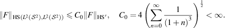
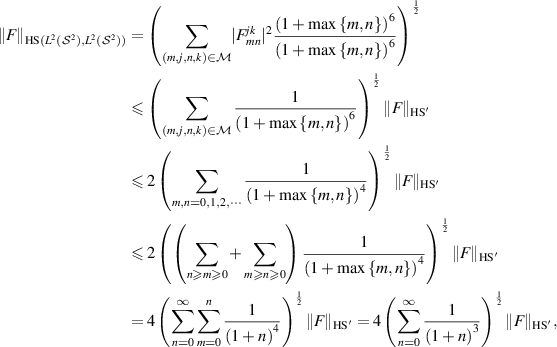
Remark B.2. From the properties of the Hilbert-Schmidt norm [Con90, exercise IX.2.19(h)], one has

Recall  is the far-field operator given in (1.2).
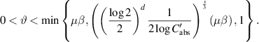
Our main strategy is to modify the ideas in [DCR03] (see also [KRS21] for more details about the mechanism). Given any ϑ > 0,  and β > 0, we consider the following set:

where Br denotes the ball or radius r centered at the origin. The following lemma verifies the assumption (a) of [DCR03, theorem 2.2], can be proved as in [Man01, lemma 2] (we omit the proof), see also [Isa13, KUW21, KW22, ZZ19]. We refer [KT61] for a version in a more abstract form.
Lemma B.3. Fix  and
and  . There exists a constant
6
. There exists a constant
6
 such that the following statement holds for all β > 0 and for all
  : there exists a ϑ-discrete subset
  of
of  7
such that
7
such that

In addition, all elements in  are in
  .
.
Similar to [DCR03], the proof of theorem B.1 is quite delicate, which is not an obvious consequence of the abstract theorem in [DCR03, theorem 2.2]. From the asymptotic expansion (1.1c ), it is easy to see that

A crucial point is to bound  for all
  , by some constant which is independent of θ and q, like [DCR03, (4.21)]. From now on, for simplicity, we restrict ourselves for the case when d = 3. We now prove the following lemma.
Lemma B.4. Let κ > 0 and let  with
with  . Then there exists a constant
  such that the following uniform decay estimate holds:
Proof. This lemma is an easy consequence of (A.6) and [Ron03, lemma 3.2] (with R = 1). □
As in [HH01], we introduce the following index set

Let  be the set of spherical harmonics. For each
  , we denote
  . Accordingly, we write

Lemma B.5. Let κ > 0 and let  with
with  . Then there exist constants
  and
and  such that

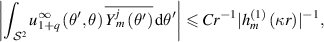
Proof. By [CK19, theorem 2.15], we can write
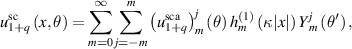
where  is the spherical Hankel function of the first kind or order m. In fact,

see the proof of [CK19, theorem 2.16]. For each  , also from [CK19, theorem 2.16], we have the following expansion
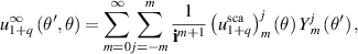
which converges uniformly in  , and hence

for all r > 1. We now combine (B.3) with lemma B.4 to obtain
uniformly in  . We now choose
  and reach

From [KW22, (48)], we see that

In view of the quantitative Stirling's formula [Rob55], we obtain
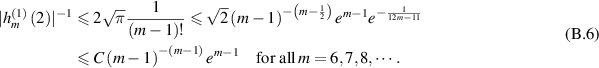
From (B.5), it is clearly that

Combining (B.4) and (B.6) implies
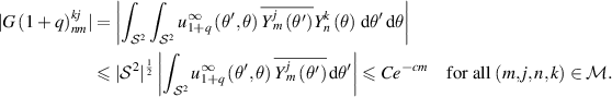
Finally, by the first reciprocity relation [CK19, theorem 8.8], we have

and the lemma is proved. □
We also need a technical lemma.
Lemma B.6. Consider the normed space

where
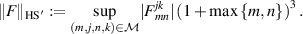
Then

we can estimate
which implies the lemma. □
We now construct a δ-net by following the procedures in [DCR03, lemma 2.3].
Lemma B.7. Let  . Then there exists a constant
  such that: for each
  we can find a δ-net
8
we can find a δ-net
8
 for
for  such that

Proof. Fix  . Let
. Let  be the smallest positive integer such that

where  and
and  are the absolute constants appeared in lemma B.5. One sees that there exists an absolute constant C > 0 such that

We define a finite subset of the complex plane  by
by
It is easy to see that
We now define the set

Let  be the number of
  such that
  , then we have

Plugging (B.10) and (B.11) into (B.12) yields
and, furthermore, from the trivial estimate  for all
  , we see that
which gives (B.8).
The remaining task now is to verify that the set  constructed above is a δ-net for
  . Fix
. Fix  and consider the far-field pattern
  . For each
  with
with  , we choose
  be the closest element to
  ; otherwise for those
  with
with  , we simply choose
  . We define the operator
  by
by

By lemma B.5, we see that
Therefore, if  , we have that

Otherwise, when  , from lemma B.5 and (B.9), we estimate

Consequently, by lemma B.6, we finally obtain

□
We are now ready to prove the main instability estimate by combining lemmas B.3 and B.7.
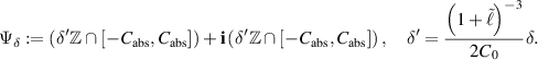
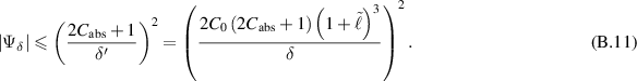
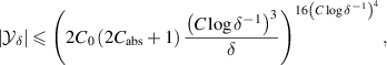
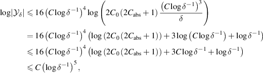
Proof of theorem B.1. Let  and
and  be the constant obtained in lemma B.7. We choose
  such that

where  is the constant given in lemma B.3 (with d = 3). Let us pick ϑ satisfying
Assume that the set  is given in lemma B.3 (also take d = 3). Next we choose
and construct the  described in lemma B.7. Since
  , it is clear that
  is also a δ-net for
  . Moreover, we can check that
Combining (B.2), (B.8) and (B.13) implies

This enables us to choose two different  (by definition of
  it holds that
  ) such that there exists
  such that

which proves the theorem by using (B.1). □
Footnotes
- 6
In fact, one can choose
for some with . - 7
This means that
for all . - 8
This means that for each operator
there exists which is approximate F0 in the sense that .