

Abstract
We propose an approach to detailed balance violation in electrical circuits based on the scattering matrix formalism commonly used in microwave electronics. This allows us to easily include retardation effects, which are paramount at high frequencies. We define the spectral densities of phase space angular momentum, heat transfer and cross power, which can serve as criteria for detailed balance violation. We confirm our theory with measurements in the 4–8 GHz frequency range on several two port circuits of varying symmetries, in space and time. This validates our approach, which enables straightforward treatment of quantum circuits at ultra-low temperature.
Export citation and abstract BibTeX RIS

Original content from this work may be used under the terms of the Creative Commons Attribution 4.0 license. Any further distribution of this work must maintain attribution to the author(s) and the title of the work, journal citation and DOI.
Corrections were made to this article on 8 April 2024. The abstract was amended for clarity.
1. Introduction
There has recently been a fast-growing interest in the thermodynamics of simple, small systems, particularly through the study of heat engines [1–4] or particles driven by noise sources [5], such as Brownian motion in a fluid [6]. A particular effort has been devoted to electrical circuits, in which the variables such as position or velocity of the Brownian particle are replaced by macroscopic variables in the circuit, such as charge or voltage across a capacitor, and where the noise is the Johnson–Nyquist thermal noise of resistors [7–9]. All these systems, from biological entities to electrical circuits, may indeed obey similar equations of motion.
The simplest and most intensively studied circuit consists of two capacitors coupled to two resistors through another capacitor. Even a simple circuit such as this shows non-trivial heat transport [10–13], gyration and detailed balance violation [8, 9]. Most studies have been performed within the framework of classical physics. However, there is currently a huge development in quantum technologies and circuits, understanding the thermodynamic properties of which are of utmost interest. It is thus crucial to extend the methods developed in classical circuits to quantum ones [14, 15].
A prerequisite for studying circuits in the quantum regime is to work at frequencies  with T the temperature [16]. Since a temperature T = 1 K corresponds to a frequency
  GHz, experiments are usually performed below 1 K in the microwave domain. Since circuits are usually larger than the wavelength, retardation effects are paramount. Unfortunately, previous studies in classical circuits have focused on circuits composed of lumped elements for which propagation times have not been considered [8, 9, 15]. These approaches can probably be extended to include retardation by the addition of an infinite network of inductors and capacitors, and thus an infinite number of coupled differential equations, at the cost of an increase in complexity. The goal of the present paper is to provide a simple theoretical approach where propagation is included from the very beginning and to test it with experiments in the microwave regime.
The rest of the paper is structured as follows: section 2 is the theory, where we introduce the scattering matrix formalism and express the metrics for detailed balance violation in terms of this framework. Section 3 goes over the experimental setup used to test our theoretical predictions in the microwave regime. Section 4 presents the experimental data, while we conclude in section 5
2. Theory
Detailed balance refers to the absence of probability currents in phase space. This can be demonstrated using global metrics such as heat current and angular momentum in phase space. Below we derive expressions for these quantities when the system is described by a scattering matrix in the frequency domain.
2.1. Scattering matrix formalism
We consider linear circuits where the current and voltages are simply related by a frequency-dependent impedance matrix. Measuring voltages (respectively currents) requires high (low) impedance sensors, which are difficult to implement at high frequencies. One would rather work with matched amplifiers, i.e. amplifiers whose input impedance is the same as that of the transmission line connected to it, so that all the power sent to the amplifier is absorbed. Such amplifiers do not measure the voltage at a point in the circuit but the amplitude of the wave incoming to them. We will focus on matched amplifiers and briefly discuss the case of voltmeters. We chose to work, as usual in microwave electronics, with the scattering formalism [17]. In this formalism, a circuit connected to n ports is modeled by an n × n matrix and the scattering matrix S, which relates the amplitude of the voltage waves exiting each port to that entering each port. Sources appear as incoming waves and measurements can be performed on each outgoing wave.
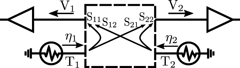
In the following, we will apply the scattering formalism to a simple yet nontrivial circuit, which contains only two ports, i.e. two noise sources and two measurements, as shown in figure 1. This situation is very close to the one usually considered at low frequency [8–11]. We have implemented this setup experimentally, as we show below. More complex circuits can be easily treated following the same lines. We assume that the circuit is lossless and linear. Losses can be implemented by adding extra ports in which power exits the circuit. According to the fluctuation–dissipation theorem, losses must be accompanied by noise, i.e. extra noise sources must be added accordingly, which enter the circuit through the extra ports. Nonlinearities can complexify the physics a great deal, since different frequencies are coupled, and the usual scattering formalism does not apply to such systems. We do not consider nonlinearities, so the voltage measured at a given frequency depends only on noise sources at the same frequency. As a consequence, we can deal with the spectral densities of the various quantities we are considering and not necessarily their integral over a certain bandwidth.

Figure 1. (a) Two matched resistors of value R0 at temperatures T1 and T2 and emitting voltage noises η1 and η2, respectively. Both noises act as inputs into a two-port circuit represented by its four scattering parameters, while V1 and V2 correspond to the measured outputs.
Download figure:
Standard image High-resolution imageFollowing figure 1, we note  and
and  the voltage amplitude of the waves emitted by the noise sources at frequency f, and
  ,
,  the measured amplitudes of the waves leaving the circuit. They are related by:


where Sij
are the frequency-dependent elements of the S matrix. For the sake of simplicity, we suppose that the noise sources are uncorrelated and of spectral density  . Here, R0 is the impedance of the sources, which are matched to the transmission lines connected to the two ports of the circuit (for simplicity, we take the same R0 for both sources). Ti
is the (possibly frequency-dependent) noise temperature of the source i. If the noise sources are resistors in the classical regime, Ti
is simply their thermodynamic temperature [18, 19]. If they are resistors in the quantum regime, the noise temperature Ti
is related to the thermodynamic temperature
. Here, R0 is the impedance of the sources, which are matched to the transmission lines connected to the two ports of the circuit (for simplicity, we take the same R0 for both sources). Ti
is the (possibly frequency-dependent) noise temperature of the source i. If the noise sources are resistors in the classical regime, Ti
is simply their thermodynamic temperature [18, 19]. If they are resistors in the quantum regime, the noise temperature Ti
is related to the thermodynamic temperature  by
by  .
.
Below, we focus on two questions: (i) How can we compute the interesting physical quantities introduced in previous work, such as heat transfers and fluctuation loops [8], using our approach? (ii) Can we find a better way to determine if the circuit is out of equilibrium?
2.2. Heat transfers
A great deal of work has been devoted to the heat transfer between two capacitively coupled resistors [10–13]. Similar quantities can be calculated using the scattering formalism. Following [10], we note  as the electrical power dissipated in the resistor at port 1. It is given by the product of the voltage across that resistor,
  , with the current flowing in it,
  [10, 17]. Since this quantity is nonlinear in voltage, it mixes frequencies: its spectral density involves a convolution in frequency space. However, the spectral density of the average power
  is well defined, given by:

This has a clear interpretation: it corresponds to cooling of the resistor by emission of a wave of amplitude η1 and heating by the absorption of a wave of amplitude V1. It corresponds to the net power transfer from the left part of figure 1 into the circuit. Introducing the detected power spectral densities  and their difference by
  , we find:

This result is a generalization of what has been obtained at low frequencies, see equation (16) of [7]. Thus, Δp is a measure of the heat current, which vanishes at equilibrium. This also means that, for any circuit, there cannot be a difference between the two detected power spectral densities unless  , provided that
  , i.e. the circuit must not divide the power equally, in which case Δp always vanishes. From the heat current one can compute the spectral density of the average entropy production per unit time,
  [10].
[10].
2.3. Angular momentum and stochastic area
It was demonstrated in [8, 9] that fluctuation loops are observed in out-of-equilibrium circuits. These loops are closed trajectories in the (V1,V2) plane, characterized by a stochastic area A. The existence of fluctuation loops corresponds to an average rotation of (V1, V2), to which is associated an angular momentum along the perpendicular axis given by:

It is simply related to the stochastic area by  . This reads in Fourier space:

with  the angular momentum spectral density. For purely white noise,
  could diverge at high frequency. Experimentally, the integral will have finite bounds due to the finite bandwidth of the circuit and divergences never occur (in other terms, the measured voltage is continuous and has a well-defined time derivative). We find:

Thus the cross-correlation between V1 and V2 is a measure of the angular momentum, which vanishes at equilibrium. Indeed, we find:  with
with  . This means that, for any circuit, there cannot be any correlation between the two voltages detected, unless
  . The only condition is β ≠ 0, i.e. the circuit must have a finite transmission. The condition on the angular momentum is, however, more stringent because of the imaginary part: if β is real, then
  . This remark sheds light on the simple reason why there are loops: the circuit must introduce a phase difference between the two branches, so that for each frequency, the two noise sources generate a rotating point in the
  plane. Due to the unitarity of the S matrix, the two rotate in opposite directions and, if the amplitude of the two noise sources is equal, there is no global rotation. The overall direction of rotation depends on the sign of ΔT as well as the sign of the phases in the S matrix.
2.4. Cross power
The difference in auto-correlations and the cross-correlation of the detected voltage can be used to detect deviations from equilibrium. Experimentally, these two quantities can be affected by imperfections: the first is sensitive to asymmetries in the detection (amplitude mismatch) and amplifier noise, while the second is sensitive to phase mismatch due, for example, to a difference in cable lengths. The angular momentum appears to be related to the in-quadrature part of the cross-correlation  and with a weighting factor f. The absolute phase of
  is not essential to determine if the circuit is out of equilibrium: changing the length of a measurement cable rotates the phase of β, which may make
  change sign or vanish. The frequency-dependent weighting factor in lz
is also of no importance for determining whether the circuit is at equilibrium or not, since all frequencies are equal for that purpose. Thus, from a practical point of view it might be interesting to define the cross-correlation power spectral density as
change sign or vanish. The frequency-dependent weighting factor in lz
is also of no importance for determining whether the circuit is at equilibrium or not, since all frequencies are equal for that purpose. Thus, from a practical point of view it might be interesting to define the cross-correlation power spectral density as
where we take the modulus of the cross correlation to remove the phase problem. We find:  . This quantity is clearly a valid metric of ΔT that is immune to amplifier noise and cable lengths. However, it does not allow us to find out which source is hottest.
3. Experimental setup
We have performed a thorough experimental test of our theoretical results. Beyond checking the formulas, the goal was to demonstrate the following prediction that emerges from our calculations: breaking spatial and/or time reversal symmetries cannot generate heat current or angular momentum, only ΔT matters. For this, we performed measurements on circuits with various symmetries, see the bottom of figure 2. Note that, while spatial symmetry has already been considered in previous work, time-reversal symmetry cannot be probed since propagation times are neglected.
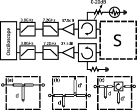
Figure 2. (Top) Experimental setup. The dashed box represents the coupling circuit of scattering matrix S. (Bottom) All three coupling circuits used to test different S matrices.
Download figure:
Standard image High-resolution imageThe experimental setup is shown in figure 2. All measurements have been performed at room temperature using a variable attenuator and a calibrated noise source as the hot source (T1 adjustable between 290 K and 560 K) and a 50 Ω resistor at room temperature as the cold source (T2 = 290 K). We have chosen to work in the 4–8 GHz frequency range, which is similar to many other experiments performed in the quantum regime at ultra low temperatures. The noise source and 50 Ω resistor, with a bandwidth of 18 GHz, can be considered white over the measurement bandwidth. The separation between incoming and outgoing waves is achieved using two circulators: the signals emitted by the sources are injected in the circuit and not in the related amplifiers, while those leaving the circuits enter the amplifiers and are not lost in the sources. Moreover, the noise emitted by the amplifiers is absorbed by sources that are matched to the microwave circuit. This minimizes parasitic cross-correlations. Given the noise temperature  K of the amplifiers and isolation of the circulators, we estimate the parasitic contribution of
  K (more circulators can be used if needed). After amplification and filtering to keep the signal within a well-defined bandwidth, the signals are digitized using a 20 GHz, 40 GS s−1, 8 bit digital oscilloscope. The time series are acquired in batches of 2 MS that are split into chunks of 2048 points. Spectra are then calculated using a discrete Fourier transform on each chunk. We then calculated the auto- and cross-correlations using these spectra and averaged over all the chunks. The size of the chunk sets the frequency resolution, here 20 MHz, which is sufficient for the circuits under consideration.
In order to test the effect of spatial/time reversal symmetries, we have studied the three circuits shown in figure 2. The circuits are made of pieces of coaxial cables of various lengths connected by T-junctions and terminated by open or short circuits. The lengths  of 5.08 and 7.62 cm, respectively, are chosen so that reflections of waves at the ends of the cables and at the junctions provide rich interference patterns that result in strong frequency-dependence of the S-matrix, thus providing a thorough test of our theoretical results, see the dashed lines in figure 3. Here, the propagation times are essential. Circuit (a) in figure 2 is symmetric upon exchange of ports 1 and 2 while circuit (b) is not. Circuit (c) contains a circulator in order to break time-reversal symmetry. In order to make a quantitative comparison between our predictions and the measurements, we have measured the S matrix of all three circuits using a vector network analyzer (VNA), see the dashed lines in figure 3.
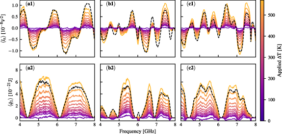
Figure 3. (a1) (resp. (b1) and (c1)): measured average spectral density of angular momentum for the circuit of figure 2(a) (resp. (b) and (c)) as a function of frequency in the 4–8 GHz range. Different colours correspond to different temperature differences according to the color bar on the right. The dashed lines represent the prediction of equation (7) using the measured scattering parameters and  K. It is thus proportional to
 ![$f\mathrm{Im}[S_{12}S_{22}^*]$](https://content.cld.iop.org/journals/1742-5468/2024/3/033206/revision5/jstatad2dd8ieqn34.gif) . (a2) (resp. (b2) and (c2)): measured average power spectral density for the circuit of figure 2(a) (resp. (b) and (c)) as a function of frequency in the 4–8 GHz range. Different colours correspond to different temperature differences according to the colour bar on the right. The dashed lines represent the prediction of equation(4) using the measured scattering parameters and
. (a2) (resp. (b2) and (c2)): measured average power spectral density for the circuit of figure 2(a) (resp. (b) and (c)) as a function of frequency in the 4–8 GHz range. Different colours correspond to different temperature differences according to the colour bar on the right. The dashed lines represent the prediction of equation(4) using the measured scattering parameters and  K. It is thus proportional to
  .
.
Download figure:
Standard image High-resolution image4. Results
In figure 3, we show the spectral densities of the angular momentum  (top) and transferred power
  (bottom) as a function of frequency for the three circuits of figure 2. The two quantities exhibit strong oscillations vs. frequency that orginate from interference occurring due to total reflections at the ends of the cables and partial reflections at the junctions between them. We observe a very good quantitative agreement between the measurements and theoretical predictions of equations (4) and (7), shown as dashed lines in figure 3. These have been obtained using the measured coefficients of the scattering matrix and the calibrated noise temperature of the hot noise source. We attribute the small differences between theory and experiment to experimental imperfections; in particular, the lack of reproducibility of connections/disconnections between the VNA and noise measurements and the losses in the cables and circulator. The slightly negative values of
  are due to the presence of amplifier noise, which is not accounted for in equation (4).
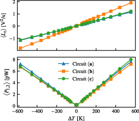
The dependence of the integrated angular momentum  and cross-power
  on the temperature difference ΔT is shown in figure 4. These curves have been obtained by integrating the spectra of figure 3 over frequency between 7.3 and 7.5 GHz for the angular momentum and the full 4–8 GHz bandwidth for the cross power (the relatively narrow bandwidth for
  has been chosen to avoid sign change leading to a vanishing
  ). The data corresponding to
  have been obtained by swapping the cold and hot sources. As predicted,
  and
and  . This is true for all circuits, i.e. is independent of the presence or absence of spatial and/or time-reversal symmetries in the system.
Figure 4. (Top) Total angular momentum in the frequency range 7.3–7.5 GHz for the three circuits of figure 2 as a function of ΔT. (Bottom) Total cross-power in the frequency range 4–8 GHz for the three circuits of figure 2 as a function of ΔT.
Download figure:
Standard image High-resolution image
We notice that  , which in theory should be proportional to
  , is experimentally not exactly a perfectly even function of ΔT. This comes from the impedances of the sources not being exactly 50 Ω, so reversing the sources also slightly changes S. The same thing happens to
  , which is not perfectly odd, although it is less obvious. For
  , we find a residual cross-power which corresponds to what we expect for
  K. We understand this as amplifier noise (
 K) being averaged over a finite number N = 100 of times. This yields
  K, in reasonable agreement with the measurement. We also find a residual angular momentum corresponding to
  K, in good agreement with our prediction, see section 3.
5. Conclusion
We have shown, both theoretically and experimentally, how heat transfer and angular momentum, quantities that have been introduced in electrical circuits at low frequencies in the context of detailed balance violation can be extended to microwave circuits where propagation delays are paramount. Our approach is very general and can be used not only for microwaves but also for guided optics, for example. In particular, it allows us to treat circuits in the quantum regime  where the noise spectra of the sources have a frequency dependence that reflects the presence of vacuum fluctuations [12].
From our results, one can recover previously obtained results at low frequencies where propagation times vanish [10, 11]. For this, one has to consider voltmeters and not only matched amplifiers. This can be done as follows: a voltmeter does not measure the outgoing voltage  but the sum of the incoming
  and outgoing voltages,
  . As a consequence, our approach is valid provided we replace the scattering matrix S by S + 1. However, the calculation needs to be redone since we have used the unitarity of the S-matrix to simplify our final formulas and S + 1 is not unitary.
We have focused on the detection of detailed balance violation using average quantities such as average heat transfer and average angular momentum. These involve the measurement of the second-order correlations of the detected voltages. Some previous works have considered the fluctuations of these quantities and calculated their probability distribution [10–12]. With our approach, it is possible to reconstruct these distributions by measuring their moments. For example, the variance of the angular momentum is related to correlations of order 4 of the measured voltages. Dealing with moments would be particularly interesting with non-Gaussian noise: what happens in a circuit with two noise sources of equal variance but opposite third moments, generated, for example, by two shot noise sources with opposite bias? Finally, recent theoretical work addresses the problem of parametrically driven circuits [15], which could be implemented using varactors or Josephson junctions, for example. Another option would be to have time-dependent noise sources, such as AC-biased tunnel junctions [20]. In such circuits, considering propagation times will be essential. However, such circuits mix frequencies and a more elaborate approach will be needed, both theoretically and experimentally.
Acknowledgments
The authors would like to acknowledge the many conversations with Clovis Farley and Simon Bolduc Beaudoin. This work was supported by the Canada Research Chair program, the NSERC, the Canada First Research Excellence Fund, the FRQNT, and the Canada Foundation for Innovation.