
Abstract
This paper follows a detection-theoretic approach for using synthetic-aperture measurements, made at multiple moving passive receivers, in order to form an image showing the locations of stationary sources that are radiating unknown electromagnetic or acoustic waves. The paper starts with a physics-based model for the propagating fields, and, following the general approach of McWhorter et al (2023 arXiv:2302.06816, IEEE Open J. Signal Process.4 437–51), derives a detection statistic that is used for the image formation. This detection statistic is a quadratic function of the data. Each point in the scene is tested as a possible hypothesized location for a source, and the detection statistic is plotted as a function of location. Because this image formation process is nonlinear, the standard linear methods for determining resolution cannot be applied. This paper shows how to analyze the detection image by first writing the noiseless image as a coherent sum of shifted complex ambiguity functions of the source waveform. The paper then develops a technique for calculating image resolution; resolution is found to depend on the sensor-source geometry and also on the properties (bandwidth and temporal duration) of the source waveform. Optimal filtering of the image is given, but a simple example suggests that optimal filtering may have little effect. Analysis is also given for the case in which multiple sources are present.
Export citation and abstract BibTeX RIS

Original content from this work may be used under the terms of the Creative Commons Attribution 4.0 license. Any further distribution of this work must maintain attribution to the author(s) and the title of the work, journal citation and DOI.
1. Introduction
This paper addresses the problem of determining the locations of stationary sources, from which are radiating unknown electromagnetic or acoustic waves, using data measured by passive receivers moving along known flight paths. Examples of sources of interest are radars and wireless communication systems 2 . The ambient medium is assumed to be homogeneous with speed of wave propagation c. Both sources and receivers are assumed to be isotropic.
This paper does not consider imaging in clutter [1], nor does it address imaging through random media [2]. Nor does it consider 'passive radar' [3–6] or 'passive coherent localization' [7] or 'hitchhiker' imaging (e.g. [8, 9]), which are systems that form images of targets using signals from sources of opportunity that reflect from the targets to the sensors. This latter problem 3 might seem similar to the source localization problem, but in fact the two problems differ significantly in their statistical formulation [4, 10].
The passive source localization problem considered here can be broken down into two components: first study (1) the statistical problem of detecting the presence of a common source signal appearing in measurements on separate receivers, and then, given the presence of a common signal, (2) determine the location of the source.
The statistical component (1) has been addressed, for example in [4, 10–14]. Some of this work includes the observation that the detection statistic involves quantities computed from a matrix of receiver cross-ambiguity functions. Two types of signal models for Component (1) are relevant for different types of sources. When the sources are random, the incoherent field approximation [9, 15] can be used, or the covariance could be modeled as in [16]. In this paper, however, we develop the theory relevant for sources transmitting deterministic (but unknown) coded signals such as chirps. Such signals are typically narrowband.
The localization component (2) has been studied from a number of points of view, including triangulation and 'two-step' methods such as [17–21], in which pairwise time-difference-of-arrivals (TDOAs) and frequency-difference-of-arrivals (FDOAs) are found first, and then the source location is obtained by solving the system of nonlinear TDOA and FDOA equations. Approaches to Component (2) alone have also been proposed that involve collecting data over a synthetic aperture [22–24]; these papers did not address Component (1). In addition, [22, 23] both made extra assumptions (orthogonality or separability) on the transmitted waveforms in order to obtain a linear imaging method.
Both components (1) and (2) are addressed simultaneously in the 'direct position determination' approach as in [25–27], in which all the data is used in a maximum-likelihood (ML) estimate for the position. The work [26], in particular, sets up the problem for a synthetic-aperture array of receivers, and observes that the ML estimation involves a matrix of cross-ambiguity functions. These cross-ambiguity functions are quadratic in the data, and consequently standard linear approaches for obtaining image resolution cannot be applied. In particular, [26] does not analyze resolution or other properties of the resulting image.
Both components (1) and (2) have also been studied together in [6, 28], which develop detectors for source localization and also form images by plotting a detection statistic, typically as a function of parameters such as delay and Doppler shift. The idea here [6, 10, 13, 14, 25–28] is that when the hypothesized parameters are correct and consequently the shifted signals are properly aligned, the detection statistic will be larger than in the misaligned case, and the resulting image will show a peak at the correct location. These detection statistics are typically nonlinear functions of the data; consequently a theoretical analysis of the resulting image is difficult.
The problem of passive source localization also occurs in radio astronomy, where it is usually addressed with large sensor arrays. The paper [24] proposes a synthetic-aperture approach using only temporal information; it is thus closely related to a multi-sensor, single-source version of [23],
The only papers to estimate image resolution are [23, 24]; but these papers did not address the issue of noise. The approach of [23] required various extra assumptions to convert the quadratic imaging method to a linear method, to which standard resolution analysis applies. In the present paper, on the other hand, we develop a method for obtaining resolution for the nonlinear synthetic-aperture approach.
The new contributions of the present paper are the following.
- (i)We develop a synthetic-aperture passive source localization (SAPSL) algorithm that, unlike the previous synthetic-aperture approaches [22, 23], is based on a solid statistical foundation. This work answers the questions implicit in [22, 23] regarding whether it is better to start with a cross-correlation or a cross-ambiguity function, and how measurements with widely different noise levels should be handled.
- (ii)We extend the prior statistical approaches [6, 10, 13, 14, 25–28] to a synthetic-aperture formulation. Our approach, which is based on the generalized likelihood ratio (GLR) approach of [10, 13, 14], is different from [6, 25–28] in which the unknown attenuation factors ('gains') are estimated first, before the unknown waveform is estimated. In this paper these gains are assumed to be known; in other words we separate the imaging problem from the 'autofocus' problem. Thus we study the imaging problem in which the sensor positions are known and the system is well-calibrated and synchronized. We treat the autofocus problem in a separate paper.
- (iii)This paper is the first to show how the full SAPSL point-spread function, which is a sum of shifted ambiguity functions, can be expressed as an integral over wavenumber space or ' k -space'. This is nontrivial because the imaging algorithm depends quadratically on the data. This analysis, moreover, can be applied also to other problems (e.g. [29]) in which the image is expressed as a sum of ambiguity functions.
- (iv)This paper is the first to provide a comprehensive resolution analysis for the full nonlinear SAPSL method. Here resolution is defined as the width of the point-spread function. This resolution analysis is an extension of the analysis in [23], which studied a linearized version of the method for the case of broadband waveforms.We provide some examples of the resolution calculation for a simple representative geometry.
- (v)This paper provides an optimal imaging filter. This was done in [23] only under the linearizing approximations; it is not done in any of the other previous work on passive source localization.
- (vi)This paper addresses the issue of redundant information (overlapping regions in k -space) in the data. This is also new.
- (vii)
The paper is organized as follows.
- Section 2 sets out the mathematical model and assumptions.
- Section 3 derives the image formation method, following the development of the detector developed in [13, 14].
- Section 4 analyzes the image formed by the method in section 3; this section contains the new results. Each of the four subsections derives a new result.The first subsection is concerned with resolution: we show how to express the point-spread function in terms of the k -space data collection manifold, and from the data collection manifold, we derive resolution. We provide explicit resolution formulas for an example of a simple representative geometry; the resolution formulas of [23, 24] are special cases.The second subsection shows how to determine an optimal imaging filter; the third subsection discusses the case in which the data collection involves redundant information (overlapping regions in Fourier space); the fourth subsection analyzes the case of multiple sources.
- Section 5 summarizes the conclusions and directions for further work.
- The paper concludes with three appendices containing details of certain calculations and a detailed discussion of figure 4.
2. Mathematical model
We consider sources located at unknown positions  , each transmitting an (unknown) waveform of the form
 ![$\psi_{\boldsymbol{x}_j}(t) = \hbox{Re} \left[ e^{i \omega_j t} a_{\boldsymbol{x}_j} (t) \right]$](https://content.cld.iop.org/journals/0266-5611/40/5/055003/revision2/ipad3165ieqn2.gif) . Here ωj
denotes the angular carrier frequency for the source j and
. Here ωj
denotes the angular carrier frequency for the source j and  is the complex baseband signal transmitted from location
x
j
. Consequently the overall time-varying source distribution is
is the complex baseband signal transmitted from location
x
j
. Consequently the overall time-varying source distribution is  .
.
We assume that all the transmitted signals are narrowband, which means that they are each of the form ![$\hbox{Re} \left[ e^{i \omega_0 t} a (t) \right]$](https://content.cld.iop.org/journals/0266-5611/40/5/055003/revision2/ipad3165ieqn5.gif) , where the bandwidth of the complex baseband signal a(t) is small relative to the carrier frequency ω0. Typical examples are the signals transmitted by weather radars and airport surveillance radars. These systems typically transmit at S-band (
, where the bandwidth of the complex baseband signal a(t) is small relative to the carrier frequency ω0. Typical examples are the signals transmitted by weather radars and airport surveillance radars. These systems typically transmit at S-band ( 2 - 3 GHz), with pulse duration on the order of 1–100 microseconds, with bandwidth of a few MHz, and pulse repetition frequency of about 1 kHz. These signals, as well as most wireless communications signals, are all narrowband.
The transmitted waves are assumed to propagate through a homogeneous medium with speed c. Here we model propagation of electromagnetic waves with the scalar wave equation

The waves are received by L sensors moving along known trajectories  , so that the signal at sensor
  is then
  , which is given by
where  ,
,  , and, for the isotropic sources considered in this paper,
  . We assume that all sensor clocks are synchronized.
The goal is to determine the locations
x
j
from the data  . We assume we know the receiver trajectories
  and associated velocities
  , but the waveforms aj
are unknown, as are the ranges
, but the waveforms aj
are unknown, as are the ranges  and time delays
  . A model similar to (2) applies to the case of moving sources, but typically then the source velocities are also unknown.
We note that this is a nonstandard type of inverse problem, in that the forward map (2) from  to
to  requires knowledge not only of the source positions, but also of the waveforms transmitted from those positions. The linear inverse problem of determining
  from
from  , however, would be severely underdetermined.
We begin by assuming that some method (e.g. [30–32]) has been used to estimate one of the carrier frequencies, say ω0. If the estimate is slightly wrong, we merely redefine  to include the extra factor of
  .
.
We then demodulate [33–35] the signal (2) by the carrier frequency ω0, obtaining a complex signal model in which all sources transmitting at frequency ω0 are converted to baseband:

The noise term in (3) is different from that in (2); in particular, not only have we removed the carrier frequency, but we have also lumped the signals from sources transmitting at frequencies other than ω0 into 'noise'. This is not necessarily the best possible way to treat all possible interfering signals, but this assumption makes the analysis tractable. Exploration of other approaches is left for future work.
Depending on the speed with which the receiving antennas move, the sensor geometry typically changes on the order of seconds, which is a factor of 106 to 1010 greater than the period of the oscillatory carrier wave, a factor of 104 greater than a typical radar pulse duration, and a factor of 103 greater than typical pulse repetition intervals. In order to isolate individual pulses or groups of pulses and 'freeze' the geometry, we extract a snippet of the data around the 'slow time'  , say by multiplying by a smooth window (see figure 1). For example, for a radar with a pulse repetition frequency of 1 kHz, a suitable time window might have duration 10−3 seconds, so that each window would capture the response from a single pulse
4
. A similar windowing operation can be applied to non-pulsed signals, such as communications signals. The windows, taken together, can form a partition of unity, so that no data is lost.
, say by multiplying by a smooth window (see figure 1). For example, for a radar with a pulse repetition frequency of 1 kHz, a suitable time window might have duration 10−3 seconds, so that each window would capture the response from a single pulse
4
. A similar windowing operation can be applied to non-pulsed signals, such as communications signals. The windows, taken together, can form a partition of unity, so that no data is lost.
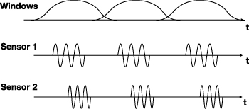
Figure 1. This shows a notional diagram of radar data measured on two sensors and possible windows that could be used to introduce the slow time parameter sm . The signals measured at the two sensors are time-shifted and Doppler-shifted relative to each other. The source localization problem is to determine from this data, together with knowledge of the sensor trajectories, the location of the source. This diagram is not drawn to scale; typical radar systems have much more rapid oscillations and much longer gaps between pulses.
Download figure:
Standard image High-resolution imageIn the window corresponding to slow time sm , we make the Taylor expansion

where  , etc. This expansion induces the corresponding expansion in τ:

We note that  is of order
  , where v is a sensor velocity, and is consequently small; it can be neglected in the argument of the slowly varying function aj
but must be retained in the exponent where it is multiplied by a large frequency. We introduce the 'slow time' reference points sm
, and then make the 'fast time' change of variables
, where v is a sensor velocity, and is consequently small; it can be neglected in the argument of the slowly varying function aj
but must be retained in the exponent where it is multiplied by a large frequency. We introduce the 'slow time' reference points sm
, and then make the 'fast time' change of variables  in (3):

where we have used the fact that aj
is slowly varying to neglect the term  in the argument. Here
  , which for an isotropic source is

where  . We note that
  is nonzero and is independent of the fast time t.
In (6), we write  , write
  for the angular Doppler-shift frequency, and drop the tildes, to obtain the baseband data model

The sum over j is only over those sources that are transmitting at carrier frequency ω0. For sources such as radars, which typically transmit repeated pulses, and windows chosen to correspond to those pulses, the mth baseband waveform  corresponds simply to the mth pulse transmitted from location
x
.
corresponds simply to the mth pulse transmitted from location
x
.
3. Derivation of the imaging formula
Our approach is similar to that of [26], except that instead of the maximum likelihood, we use the GLR detection statistic derived in [10, 14]. An image is formed by the following steps:
- (i)For each hypothesized source location y , we time-shift and Doppler shift the data measured at each receiver to remove the propagation effects (time delay and Doppler shift) assuming the source is at y . This process can be thought of as aligning the data.We note that the complex attenuation/gain
 , which has the assumed form (7), is also known since
y
is assumed known.
, which has the assumed form (7), is also known since
y
is assumed known. - (ii)Once the data is aligned, we apply a statistical test [equations (23), (24), and (28)], the derivation of which follows [10, 14], to determine the degree to which the aligned signals are the same. The statistic we use indicates the likelihood that a common signal is present at the various receivers. We plot the likelihood ratio as the image value at pixel y .
- (iii)We apply the same process to each hypothesized source location (image pixel) y in turn.

We describe these steps in more detail below.
3.1. Alignment of the data for a hypothesized location
For a hypothesized source position y , the time delay and Doppler shifts appearing in (8) would be

Consequently, to test  for the presence of a common signal emanating from location
y
, we apply the appropriate time advance and Doppler (un-)shift to each
for the presence of a common signal emanating from location
y
, we apply the appropriate time advance and Doppler (un-)shift to each  :
:

In terms of the data model (8), η can be written
where  and
and  are the differences

Figure 2 shows data, as measured at the sensors after it has been demodulated, time-advanced, and Doppler-shifted, due to a repeating sequence of linear chirps transmitted from the origin. The transmitted chirps have bandwidth of 1.6 kHz, center frequency of 3 GHz, duration 1 second, and a pulse repetition interval of 2 s. The processing windows are 1 second long. These parameters are chosen for visibility in the plots and not for realism. The geometry is shown in figure 3: sensor 1 starts at (−10 km,−10 km, 5 km) and moves at 360 m s−1 in the direction (1,0,0); sensor 2 starts at (0, −10 km, 5 km) and moves at the same speed in the same direction. The top row of figure 2 shows graphs of initial segments of the signals received at each of 6 slow times. The straight lines at slow times 2, 4, and 6 correspond to slow times at which no signal is received. The bottom row shows spectrograms, i.e. windowed Fourier transforms, using sliding windows much shorter than the 1-second processing window. The spectrograms are plotted on a dB scale. The dark vertical stripes in the spectrograms correspond to windows in which no signal is received; these correspond to the horizontal lines at slow times 2, 4, and 6 in the top row.
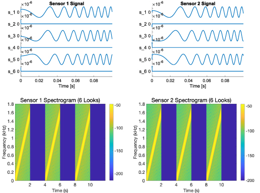
Figure 2. Signals at the sensors for a repeating sequence of chirps transmitted from the origin. The top row shows graphs of the initial parts of the time-advanced and Doppler-shifted signals (10) received at each of the 6 slow times. The bottom row shows spectrograms for 6 looks. The spectrograms are plotted on a dB scale.
Download figure:
Standard image High-resolution image
Figure 3. For each sensor,  ; and for small angles,
  .
.
Download figure:
Standard image High-resolution imageIf there is indeed a source at location y , then the frequency difference and delay difference are zero, and η becomes
where the subscript
y
corresponds to the appropriate index j for which  . The sum over j for which
  is lumped in with the rest of the noise. Thus we assume that when a source is present at
y
,
is lumped in with the rest of the noise. Thus we assume that when a source is present at
y
,

Here we are using a strategy similar to that used in active synthetic-aperture radar, where one develops an imaging algorithm based on a model for scattering from a single point-like target, even though scenes of interest typically consist of a large number of scatterers [35]. In section 4.4, we address in detail the multiple-source case.
If the flight trajectories are known precisely, then  of (14) is known from (7) with our choice of
y
and ω0. The left side of (14) is obtained from measurements, but
of (14) is known from (7) with our choice of
y
and ω0. The left side of (14) is obtained from measurements, but  on the right side is unknown. Thus the problem of determining whether a source is present at location
y
can be formulated as the problem of determining whether the signals
on the right side is unknown. Thus the problem of determining whether a source is present at location
y
can be formulated as the problem of determining whether the signals  , obtained from measurements at different sensors
  , are proportional to a common (aligned) signal
  , plus noise.
3.2. Estimation of the waveform
Under the assumption that the hypothesized source is at location
y
, we first determine an estimate of the transmitted waveform(s)  . To do this we make use of the data on all sensors for a particular slow time m, and follow the procedure below. For each m, we assemble these data into the L-dimensional vector-valued functions
  , whose
  th element is
  , and similarly for
g
m
and
d
m
. We use the superscript
, and similarly for
g
m
and
d
m
. We use the superscript  for adjoint. Here we temporarily drop the
y
subscripts and arguments.
for adjoint. Here we temporarily drop the
y
subscripts and arguments.
We assume that the noise on each sensor  is bandlimited complex Gaussian white noise with mean zero and known variance
  . With the L-dimensional vector notation
η
and
g
, and with the notation
. With the L-dimensional vector notation
η
and
g
, and with the notation  for the covariance, we write the Gaussian likelihood for
η
as proportional to
for the covariance, we write the Gaussian likelihood for
η
as proportional to

Here for each m, the t integration extends over the support of the mth time window. The integrals in (15) can be obtained by a large-bandwidth limiting process as described in section 6.4 of [36]. More details are given in appendix
To maximize (15), we minimize, for each m, the weighted mean-square error

with respect to am
, which we do by a variational argument. Thus for all perturbations  , we have

which must be valid for all complex  . Thus we obtain the pseudoinverse expression

This is the ML estimate for the waveform transmitted from hypothesized location y during the mth slow-time interval.
3.3. Derivation of the GLR detection statistic
This derivation follows [10, 14], using slightly different notation. For the hypothesized point
y
, we consider two hypotheses, namely H0, the hypothesis that the data ηm
consists only of noise, and H1, the hypothesis that the data consists of noise plus a signal  common to the sensors. The likelihoods under H0 and H1 are proportional to
The log of the likelihood ratio is  , where

The next step is to insert (18) and rearrange; the details are given in appendix

where  , and
, and  , and where
  is the L × L self-adjoint matrix

Equation (21) can be written as the sum

where
where  denotes the usual L2 inner product and the bar denotes complex conjugate. We note that (24) contains factors that automatically weight contributions of the data from sensors
  and
and  according to the (known) signal-to-noise ratios at those sensors. We note also that
  .
.
In appendix

where  is the receiver cross-ambiguity function

and where T and  are the time difference of arrival (TDOA) and frequency difference of arrival (FDOA), respectively:

In (26), the bar denotes complex conjugate.
Equation (25) shows that, as we would anticipate from e.g. [22, 26, 37, 38], the image (24) is constructed from receiver cross-ambiguity functions. Consequently, to compute the contribution to the image at each slow time, the receiver cross-ambiguity function can be computed once, and then evaluated at the computed values of TDOA and FDOA for a grid of various hypothesized points y in the image.
The image  is formed by summing over all slow times m:

We note that this image formation process depends quadratically on the data through (26).
The likelihoods in (28) are derived under the assumption that the signals are correctly aligned, or in other words, that the source is indeed located at the hypothesized location and thus  has the form (14). When this assumption is satisfied, the sum (28) is non-negative. In the following section, we investigate the case when the signals are misaligned, or in other words when the hypothesis
y
for the source position is wrong.
has the form (14). When this assumption is satisfied, the sum (28) is non-negative. In the following section, we investigate the case when the signals are misaligned, or in other words when the hypothesis
y
for the source position is wrong.
For sources that repeatedly transmit the same waveform, as many radar systems do, there is a possibility that a signal that is time-shifted and Doppler-shifted to correspond to a signal from a distant location
y
might allow the mth pulse at the receiver to align with the  st pulse from the transmitter. This could result in image artifacts that are related to the range ambiguities that can occur in an active radar system and which can be predicted from the pulse repetition frequency of the radar. In active radar, such ambiguities can be handled by design of the antenna beam pattern so that the ambiguities are not illuminated, or by design of the sequence of transmitted waveforms so that targets at ambiguous ranges have negligible reflected energy. Here we assume that the image region is adequately restricted
5
so these ambiguities do not occur.
st pulse from the transmitter. This could result in image artifacts that are related to the range ambiguities that can occur in an active radar system and which can be predicted from the pulse repetition frequency of the radar. In active radar, such ambiguities can be handled by design of the antenna beam pattern so that the ambiguities are not illuminated, or by design of the sequence of transmitted waveforms so that targets at ambiguous ranges have negligible reflected energy. Here we assume that the image region is adequately restricted
5
so these ambiguities do not occur.
4. Image analysis
To determine the fidelity of the image, into (24) we insert the signal model (11). The strategy [35] is to analyze the image by examining its Fourier transform and discovering which Fourier components are determined by the measured data. To do this, we can consider the contributions from each sensor pair, and then add those contributions together coherently.
For simplicity we consider the case of only a single source at location x . We note that because of the quadratic nature of the image formation process, the image of multiple sources is not simply a sum of single-source images. Instead, there are cross terms, which we study in section 4.4. A special case of a similar problem was studied in [23].
The contribution to the image at
y
from a single sensor pair  and a single slow-time index m is
  , which, from (24) and (11), is
where the delay and Doppler differences at sensor  from points
x
and
y
are
from points
x
and
y
are

In (29), we make the change of variables  . This results in
where

is the classical (narrowband) radar ambiguity function, where
with
where more details are given in appendix
We note that when  , the quantities
  , and
, and  are all zero, and consequently the diagonal elements
  depend only on the signal-to-noise ratio. This means that although the detection statistic is affected by the diagonal terms, the image resolution is determined only by the off-diagonal terms of
  .
.
4.1. Resolution
To determine resolution, we examine the image (28) for y near the true source location x and determine the width of the peak in the image. To do this, we examine each contributing term (31). The strategy, as is common with many other inverse problems, is to express the image in terms of its spatial Fourier components, i.e. its wavenumber space or ' k -space'.
We write  in terms of its Fourier transform W, which is the Rihaczek distribution:

The Rihaczek distribution W is the instantaneous correlation between  and its one-term Fourier expansion
  , which we see below in (36).
4.1.1. Support of W.
For a narrowband waveform a, the support of W is determined by its duration and frequency band. We see this from the following calculation:
where A denotes the Fourier transform of a and where in the last line we have made the substitution  and carried out the
  integration. The expression (36) shows that the temporal support of a is the same as the t' support of W, and the frequency band of a (i.e. the support of A) is the same as the
  support of W.
4.1.2. Fourier components from one sensor pair.
We next expand  ,
,  , and
, and  of (37) in their Taylor series about
  , obtaining

where

Here the spatial gradients of the TDOA and FDOA are given by
where  , with the hat denoting unit vector (
 ), where
  is the sensor velocity vector at slow time m, and where the scaled projection operator
  is
is
The matrix  projects a spatial vector onto the plane perpendicular to
  . The term
  of (39) results from the expansion of
  and is given by

More details of the calculations are given in appendix
We see that the phase of (38) is of the form  . Consequently the main contribution to the integral of (38) comes from the point
  .
.
In (39), (40), and (42), we note that the vector  is orthogonal to
  for every
  and m. The terms
  and
and  of (39) can be combined as

where  is the operator that projects a vector onto the plane perpendicular to
  , so that
  . Thus each term in (43) is the ratio of the range distance R to the distance traveled perpendicular to
R
; this is the ratio of two sides of a right triangle (see figure 3) and is therefore approximately the angular aperture (in radians) covered by the sensor over the mth data collection interval. Equation (43) is the difference of the corresponding angles for the sensors
. Thus each term in (43) is the ratio of the range distance R to the distance traveled perpendicular to
R
; this is the ratio of two sides of a right triangle (see figure 3) and is therefore approximately the angular aperture (in radians) covered by the sensor over the mth data collection interval. Equation (43) is the difference of the corresponding angles for the sensors  and
and  .
.
In (38), we make the change of variables

The contribution to the image from sensor pair  and slow time m can then be written
where the Jacobian  is often called the 'Beylkin determinant' [39] and where
  is the characteristic function of the set

The set  is the set of image Fourier components, of the image near
  , determined by measurements on sensor pair
  at slow time index m. An example of a set
  is shown in figure 4.
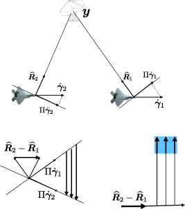
Figure 4. The top subfigure shows an example of the geometry; the lower left subfigure shows the relevant vectors in
k
-space; the lower right figure shows how these vectors are added together in (39) to produce the set  , which is the shaded blue region.
Download figure:
Standard image High-resolution imageThe union of these sets,

we call the data collection manifold (DCM) [35]. As we see below, resolution at y is mainly determined by the size of this DCM, which is determined by the set of values of Ψ of (39).
4.1.3. Combining data from all sensors.
The full likelihood image is the coherent sum of the images from each sensor pair and every slow time. In the neighborhood of the image point  , the image can be written:

where the amplitude Ξ is

4.1.4. Resolution formulas.
The resolution at
y
is determined by the data collection manifold  because the image (48) at
y
is the Fourier transform (of Ξ) over the region
because the image (48) at
y
is the Fourier transform (of Ξ) over the region  in Fourier (
k
-)space. For a source distribution consisting of a single isotropic point source at
y
, we determine the resolution of its image (the point-spread function) by noting that
in Fourier (
k
-)space. For a source distribution consisting of a single isotropic point source at
y
, we determine the resolution of its image (the point-spread function) by noting that

has a main-lobe peak-to-null width of  . Consequently, if
  extends, in direction
  , from
  to
to  , then the point-spread function will have peak-to-null resolution in direction
  of approximately
  .
.
For the geometry shown in figure 3, we refer to the direction from the sensors to the top of the page as the 'range' direction, and the direction of travel as the 'cross-range' direction. We see in figure 4 that the direction  is roughly in the cross-range direction.
Figure 4 is a sketch of the corresponding values of Ψ, as defined in (39). A detailed discussion of figure 4 appears in appendix
The resolution for the geometry of figure 4 is obtained as follows.
- Resolution from the TDOA term of (39) (relevant for short waveforms with significant bandwidth). This analysis is the same as that in [23, 24].
- 1Cross-range resolution. From the first (TDOA) term of (39), we see that the extent in direction is determined by , as ranges over the angular frequency band of the source. Consequently the single-look peak-to-null resolution in the cross-range direction is , where B is the source bandwidth in Hertz.The cross-range resolution is not appreciably affected by a small synthetic aperture (see figure 6).
- 2Range resolution. As the sensors move along the flight path, the vector rotates. With the small-angle approximation (for the aperture α), the vertical (range) extent is approximately , which gives rise to resolution of .
- Resolution from the FDOA term of (39) (relevant for waveforms of significant duration).
- Range resolution. The FDOA term of (39) is a vector that is roughly perpendicular to . Its extent, as discussed below (43), is roughly , where is the difference of angular apertures covered by the sensors. Consequently the single-look peak-to-null resolution in the range direction is approximately , where f0 is the center frequency in Hertz.Again, as the sensors move along the flight path to angle α, the single-look contributions to the DCM rotate to the angle α. With the small-angle approximation for α, the total vertical (range) extent of the DCM is roughly . Consequently the range resolution is .
- Cross-range resolution. The cross-range resolution deriving from the FDOA term arises mainly from the dwell and the synthetic aperture. The horizontal (cross-range) extent is approximately , which is the single-look vertical extent multiplied by . Consequently the cross-range resolution is approximately .
- Range resolution. The FDOA term of (39) is a vector that is roughly perpendicular to


![$c/[f_0(\theta_2 - \theta_1)]$](https://content.cld.iop.org/journals/0266-5611/40/5/055003/revision2/ipad3165ieqn142.gif)
![$\omega_0[ \alpha + (\theta_2 - \theta_1)]/c$](https://content.cld.iop.org/journals/0266-5611/40/5/055003/revision2/ipad3165ieqn143.gif)
![$ c/[f_0 (\alpha + \theta_2 - \theta_1)]$](https://content.cld.iop.org/journals/0266-5611/40/5/055003/revision2/ipad3165ieqn144.gif)


![$c /[f_0 \alpha (\theta_2 - \theta_1)]$](https://content.cld.iop.org/journals/0266-5611/40/5/055003/revision2/ipad3165ieqn147.gif)
These formulas are listed in table 1. Data collection geometry significantly different from that of figure 3 may result in different formulas. For example, one stationary sensor and one moving sensor might provide desirable resolution properties.
Table 1. Approximate resolution for geometry of figure 3. B is the bandwidth in Hertz and α is the total viewing aperture.
| Range | Cross-range | |
|---|---|---|
| Single look |

|

|
| Aperture α | min
| min 
|
4.1.5. Resolution examples
4.1.5.1. Example: an airport surveillance radar or weather radar.
We consider the resolution for a source consisting of an airport surveillance radar operating at the carrier frequency 2.8 GHz, and transmitting pulses with bandwidth  10 MHz.
The cross-range (TDOA-derived) resolution is roughly

where we have assumed that the sensor geometry is such that  . Broader-band sources provide correspondingly better resolution; sensors too close together give worse resolution.
The range (FDOA-derived) resolution, on the other hand, for data collection geometry that results in a one-degree aperture  , is approximately

An airport surveillance radar may have a narrow beam and may be rotating, so a one-degree aperture could be difficult to obtain.
4.1.5.2. Example: an X-band radar.
For an X-band radar with a 100 MHz bandwidth and center frequency of  , the cross-range resolution is approximately

and the range resolution, again for a data collection resulting in a one-degree aperture, is roughly

4.1.5.3. Example: 16 kHz bandwidth, long-duration waveform.
Communications waveforms are often long-duration and have a narrow bandwidth. In figure 5, we show the DCM and PSF for a source located at the origin, transmitting pulses of duration .08 second with (angular) center frequency  radians s−1 (≈ 1.6 MHz) and bandwidth of 105 radians s−1 (≈ 16 kHz), with sensors 50 m to the south [initially located at (−20 m, −50 m) and (20 m, −50 m)] traveling at speed 10 m s−1 along the x axis, with the geometry as shown in figures 3 and 4. (These parameters are chosen for ease of computation and for visibility of the relevant features.)
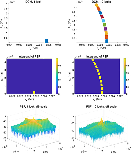
Figure 5. Resolution for a .08-second-long waveform of bandwidth ≈ 16 kHz. Top left: single-look DCM; the points in the DCM are blue, and points outside are white. Top right: 10-look DCM. The colors in the 10-look DCM plot are used to show the different sets of points from each of the 10 different looks; points outside the DCM are white. Middle left: PSF integrand for the single-look DCM directly above. Middle right: PSF integrand for the 10-look DCM directly above. Colors here indicate the value of the function defined on the DCM. Bottom: 1-look (left) and 10-look (right) normalized PSFs (these are the Fourier transforms of the functions plotted in the middle row). These are both shown in a dB scale on the vertical axis.
Download figure:
Standard image High-resolution imageThe top left plot in figure 5 is the DCM for a single look from the initial position; immediately below is the characteristic function of the DCM, which is the integrand of (57), and below that is the corresponding normalized PSF plotted with the vertical axis on a dB scale. The top right plot is the DCM for 10 looks, at slow times 0, 0.1111, 0.2222, 0.3333, 0.4444, 0.5556, 0.6667, 0.7778, 0.8889, and 1.0, as the sensors move along their trajectories. We see that the successive single-look contributions to the DCM rotate and shift counter-clockwise with successive looks. Immediately below the 10-look DCM is the characteristic function of that DCM, and below that is the corresponding normalized PSF plotted with the vertical axis on a dB scale. The units for the kx and ky axes are 1/m.
4.1.5.4. Example: 250 MHz bandwidth, short-duration waveform.
Figure 6 shows a DCM for a short-pulse waveform with bandwidth of 250 MHz around a center frequency of 2 GHz, again for the same geometry as shown in figure 3. (Again the parameters are chosen for visibility.) The different colors show the contributions for each of the 40 different looks (i.e. slow time samples). Here the contributions from different looks have minimal overlap.

Figure 6. DCM for a short-duration waveform with 250 MHz bandwidth. The contributions for the 40 different looks are each shown with a color different from that of its neighbors.
Download figure:
Standard image High-resolution imageThe resolution analysis here is similar to that of [23]. It is also similar to the analysis of standard synthetic-aperture radar (SAR) [35] except that the  in SAR is replaced here by
  , which is roughly perpendicular to the range direction
  .
.
4.2. Optimal filtering of the image
In this subsection, we follow the general strategy of [35, 40].
To the detection-based image (48), we apply a filter with kernel Q:
where we have used  . We see that to make the image as close as possible to the Dirac delta function
  , we should choose Q to be the filter

Here the  in the numerator is 1 in Ω and 0 otherwise. We note that this filter depends, in a slowly varying manner, on the image point
p
through the functions
in the numerator is 1 in Ω and 0 otherwise. We note that this filter depends, in a slowly varying manner, on the image point
p
through the functions  and the Jacobian
  . Typically the Jacobian involves a factor of
  that produces image sharpening.
With filter (56), the image (55) becomes, to leading order,

which is an approximation to a delta function located at  .
.
Thus we see that source localization is reduced to geometry and Fourier analysis. The flight trajectories, source location, and transmitted waveforms determine the set Ω, and the Fourier transform of the characteristic function of the set Ω determines the image of a single source. The connection between sets in Fourier space and associated images has been studied in [41, 42].
For k -space regions of overlap for multiple sensors and/or multiple looks m, (56) provides automatic downweighting. This is studied further in the following subsection.
4.3. Redundant information
We see in figure 7 that even a single pair of sensors can provide information that is redundant, in the sense that the k -space regions from different looks can overlap. The analysis above suggests that these overlapping regions should be downweighted by means of the filtering operation (55); but how important is this really? In figure 7 we compare the weighted PSF with the unweighted PSF for the 10-look, 1.6 kHz-bandwidth case. The weighted PSF (bottom right ) is nearly indistinguishable from the unweighted PSF (middle row, right). A close examination shows that the weighted PSF is slightly better than the unweighted one.

Figure 7. Top: A DCM in which successive time windows overlap, which results in overlapping regions in k -space. Middle left: the PSF integrand with no corrective weighting. Middle row right: the corresponding (unweighted, normalized) PSF, plotted on a dB scale. This is the Fourier transform of the function to its left. Bottom left: the PSF integrand weighted by (56). Bottom right: the normalized PSF corresponding to the Fourier transform of the function to its left.
Download figure:
Standard image High-resolution imageThe conclusion is that, at least in this case, it is the size of the k -space region that is most important for resolution, not the weighting. (And this is consistent with other numerical experiments, not shown.) In other words, data that overlaps in k -space can often be simply added together coherently, with little danger that the overlapping regions will result in appreciably degraded point-spread functions. The more overlap, of course, the more important weighting could become.
4.4. Image analysis for multiple sources
Although the image formation process was derived under the assumption that only a single source is present, in fact there may be multiple sources. This section investigates the behavior of the imaging algorithm when multiple sources are present. To do this, we insert the signal model (11) into (24):
where as before

In (58), we make the change of variables  . This results in
where

is the narrowband cross-ambiguity function, and where

Thus if the waveforms emitted at
x
j
and  have a small cross-ambiguity function, the contribution to the image of the associated cross terms will be small.
5. Conclusions
This paper has developed a statistics-based synthetic-aperture approach for forming images that show the locations of stationary sources radiating (electromagnetic or acoustic) waves, using measurements from multiple moving passive receivers. This approach is based on the detection theory of [10, 13, 14]. The resulting imaging method is nonlinear; consequently the standard linear theory cannot be used to analyze the imaging performance.
This paper, however, has also developed a method to determine the image resolution obtained from this nonlinear approach. The resolution is obtained from the data collection manifold in k -space, which gives the set of scene Fourier coefficients that can be obtained from the data. This resolution depends not only on the geometry, but also on the radiated waveforms, which are initially unknown. The resolution from multiple views is obtained by taking the union of the associated regions in k -space.
This paper also derived the optimal filtering for the image. This optimal filtering automatically downweights regions of k -space for which redundant measurements are obtained.
Finally, this paper also addressed the case of multiple sources; the image artifacts, which are due to undesirable cross terms in the nonlinear image formation process, are determined by the cross-ambiguity function of the associated waveforms. Thus, for example, a synthetic-aperture image formed of sources transmitting orthogonal waveforms will show only negligible artifacts.
The analysis in this paper may enable source-localization systems to find sources that radiate a variety of signals, including those that might radiate long-duration signals in an extremely narrow frequency band. In addition, the resolution analysis may be useful for the design and trajectory planning of systems to achieve a desired location accuracy.
We leave many related problems for the future, including addressing sources that do not radiate isotropically, source waveforms that do not satisfy the narrowband assumption, artifacts due to multiple sources radiating correlated or identical waveforms, different choices of slow times and window lengths, interference from multiple radiating sources, different noise models, use of polarimetric data, and determination of various system parameters that may be poorly known, such as the sensor positions, unknown clock offsets, and noise variances. Certain of these issues may be especially important in different specific applications. We also leave for the future the development of alternative approaches that might exploit sparsity of the sources.
Acknowledgments
We are grateful to Drs James A Given, L Todd McWhorter, and Ivars Kirsteins for many valuable discussions. This work was supported in part by the Office of Naval Research under Contract N00014-21-1-2145 and by the Air Force Office of Scientific Research 6 under the Contract FA9550-21-1-0169.
Data availability statement
No new data were created or analysed in this study.
Appendix A: Statistical fine points
A.1. Approach of [36]
To obtain (15) by the approach outlined in section 6.4 of [36], we assume that the frequency band of the noise on the  th sensor is
 ![$[-B/2,B/2]$](https://content.cld.iop.org/journals/0266-5611/40/5/055003/revision2/ipad3165ieqn170.gif) , with the flat spectrum value
, with the flat spectrum value  . Then the noise has correlation function
  where sinc
  . Samples of
  at the Nyquist times
  produce samples
  with variance
  , and the correlation between samples at times
  and
and  is
is  where
where  is the Kronecker delta. Thus such samples are independent. Over the time interval T, there are
  such Nyquist samples; their Gaussian likelihood is proportional to
 ![$(\sigma_\ell^2 B)^{-J} \exp[ - \sum_j |\eta_{\ell,m}(j/B) - g_{\ell, m} a_{m} (j/B) |^2/(\sigma_{\ell}^2 B) ] $](https://content.cld.iop.org/journals/0266-5611/40/5/055003/revision2/ipad3165ieqn183.gif) where we have used the mean in (14) and have dropped the
y
dependence. In the limit of large B, the exponential is approximated by
where we have used the mean in (14) and have dropped the
y
dependence. In the limit of large B, the exponential is approximated by  . Combining the different sensors and slow times results in (15).
An alternative approach is to use a discrete formulation for the initial steps of the derivation, as outlined below.
A.2. Estimation of the waveform am
from discrete samples of

For each slow time m and each hypothesized location y , we consider the time-sampled version of (14), which we write as

where  ,
,  ,
,  , and
, and  with
with  the noise on the
  th receiver. We assemble all the elements
  first into a column vector
  and then into a matrix
  and assemble the elements
  into a column vector
g
. Then the probability density function for
Z
is
into a column vector
g
. Then the probability density function for
Z
is

which is a more conventional discretized version of the mth factor of (19). To find
a
, we maximize
(A.2) with respect to the variables  , obtaining the pseudo-inverse
  , which is a discrete version of (18). Substituting this result into (A.2) gives

where  and I denotes the L × L identity matrix. A discrete version of the log-likelihood ratio (20) is then
At this stage we can take the limit  to obtain (21) or (B.4).
Appendix B: Detector derivation
With the estimate (18) for the waveform, the first term of (20) is
where  denotes the usual L-dimensional Euclidean norm, where

where  , and
, and  . We note that
  ,
P
, and
,
P
, and  are independent of t. Equation (B.1) can also be found in [10, 14].
Since  is an orthogonal projection and is thus self-adjoint and idempotent, the integrand of (B.1) can be written [10, 14] as
where in the third line we have used the cyclic property of trace.
Using (B.3) in (20), and writing ![$ \boldsymbol{\eta}_m^\dagger {\mathcal R}^{-1} \boldsymbol{\eta}_m = \hbox{tr } \left[ {\mathcal R}^{-1/2} \boldsymbol{\eta}_m \boldsymbol{\eta}_m^\dagger {\mathcal R}^{-1/2} \right]$](https://content.cld.iop.org/journals/0266-5611/40/5/055003/revision2/ipad3165ieqn206.gif) , we obtain
, we obtain
where  is the L × L self-adjoint matrix

We note that in the final expression of (B.4), we can drop the trace because the quantity inside the square brackets is a scalar.
Appendix C: Detector in terms of receiver cross-ambiguity
In this section we write the inner product of (24) directly in terms of receiver data.
We make the change of variables  , which is inverted as
  :
:
where  is the cross-ambiguity function of (26) and where T and
  are the TDOA and FDOA as defined in (27).
Appendix D: Resolution details
The expression for Φ is obtained as
Using Taylor expansions for  and
and  , we obtain
where, having dropped terms that are quadratic in  , we have
Appendix E: Detailed discussion of figure 4
Figure 4 is a sketch of the values of Ψ, as seen from the second equality of (39). First, the unit vectors  from the top diagram are copied to the bottom left diagram, and and their difference drawn. That gives the direction vector for the TDOA term of (39). Then that vector is multiplied by
  , where
  varies over the bandwidth of the waveform. The roughly horizontal arrows at the bottom of the bottom right plot of figure 4 shows the difference of the unit vectors
  multiplied by different lengths to represent the interval of
  factors.
The FDOA term of (39) is more complicated. First, in (43), the scaled projections  are written in terms of an actual orthogonal projection Π divided by R. When Π operates on a vector, it projects that vector onto the plane perpendicular to
  . The vector that each Π is operating on is the corresponding sensor velocity vector
  . Those projections are shown in the top diagram of figure 4, and are copied into the bottom left diagram. Then in (43), those vectors are multiplied by a scalar
  where t' ranges over the duration of the waveform. The bottom left plot of figure 4 shows those projection vectors multiplied by a scalar factor. Then (43) is the difference of those vectors for the same value of t'. Those difference vectors are represented as the downward pointing arrows in the bottom left diagram of figure 4. Those arrows all have the same direction but different lengths, ranging from a certain minimum to a certain maximum. Then, in (39), the negatives of those vectors are added to the first term. This is represented by the upward pointing arrows in the bottom right plot of figure 4: to each of the multiples of the difference of the unit vectors from the first term, we add an upward-pointing vector with a certain interval of lengths. That is represented by the blue shaded region, which is the DCM for this single look
Footnotes
- 2
Radar systems typically transmit a sequence of short pulses between which they are quiet as they listen for reflected signals, whereas communications signals are often of much longer duration.
- 3
The state of the passive radar problem is similar to that of passive source localization: statistical methods such as [3–6] have been developed for stationary sensors, and synthetic-aperture methods [8, 9] have been developed that neglect noise. Some of the latter work makes a linearizing approximation and addresses resolution of the resulting linear imaging method. Most work on passive sensing involves a cross-correlation or cross-ambiguity function.
- 4
This is consistent with standard radar processing [33–35], in which returns from each pulse are processed separately. The window should be long enough to contain multiple oscillations of the waveform, and short enough so that the changes in sensor geometry within the time window are negligible. The optimal choice of slow times and window lengths is a topic for future study.
- 5
The region of hypothesized values of y can easily be restricted. To prevent distant high-power sources from aliasing into the image region, however, it may be necessary for receivers to use a beam pattern that does not receive energy from the region of potentially ambiguous sources. More detailed investigation of this issue is left for the future.
- 6
Consequently, the US Government is authorized to reproduce and distribute reprints for governmental purposes notwithstanding any copyright notation thereon. The views and conclusions contained herein are those of the authors and should not be interpreted as necessarily representing the official policies or endorsements, either expressed or implied, of the Air Force Research Laboratory, the Office of Naval Research, or the US Government.