

Abstract
Synthetic tracking (ST) has emerged as a potent technique for observing fast-moving near-Earth objects (NEOs), offering enhanced detection sensitivity and astrometric accuracy by avoiding trailing loss. This approach also empowers small telescopes to use prolonged integration times to achieve high sensitivity for NEO surveys and follow-up observations. In this study, we present the outcomes of ST observations conducted with Pomona College's 1 m telescope at the Table Mountain Facility and JPL's robotic telescopes at the Sierra Remote Observatory. The results showcase astrometric accuracy statistics comparable to stellar astrometry, irrespective of an object's rate of motion, and the capability to detect faint asteroids beyond 20.5th magnitude using 11 inch telescopes. Furthermore, we detail the technical aspects of data processing, including the correction of differential chromatic refraction in the atmosphere and accurate timing for image stacking, which contribute to achieving precise astrometry. We also provide compelling examples that showcase the robustness of ST even when asteroids closely approach stars or bright satellites cause disturbances. Moreover, we illustrate the proficiency of ST in recovering NEO candidates with highly uncertain ephemerides. As a glimpse of the potential of NEO surveys utilizing small robotic telescopes with ST, we present significant statistics from our NEO survey conducted for testing purposes. These findings underscore the promise and effectiveness of ST as a powerful tool for observing fast-moving NEOs, offering valuable insights into their trajectories and characteristics. Overall, the adoption of ST stands to revolutionize fast-moving NEO observations for planetary defense and studying these celestial bodies.
Export citation and abstract BibTeX RIS

Original content from this work may be used under the terms of the Creative Commons Attribution 3.0 licence. Any further distribution of this work must maintain attribution to the author(s) and the title of the work, journal citation and DOI.
1. Introduction
Observing near-Earth Objects (NEOs) holds significant importance for planetary defense, solar system formation studies, and resource mining applications. While meter-size or smaller NEOs harmlessly disintegrate in the Earth's atmosphere, larger ones can cause devastating damage. The US Congress mandated NASA to find NEOs larger than 140 m with at least 90% completeness due to the potential regional devastation caused by such impacts (Brown 2005). NASA's Near-Earth Object Observations (NEOO) programs fund projects to discover, track, and characterize NEOs in response to this mandate. Currently, we have identified approximately 40% of NEOs larger than 140 m, leaving about 15,000 NEOs to be discovered (National Science & Technology Council 2023). Current surveys, such as the Catalina Sky Survey (CSS) (Christensen 2019) and Pan-STARRS (Kaiser et al. 2002), produce more than 3000 NEOs per year (https://cneos.jpl.nasa.gov/stats/site_all.html) with about 500 larger than 140 m. While the detection rate has been steadily increasing, with only the current capabilities, finding 90% of the NEOs of size 140 m or larger can easily take an extra 20 yr. Fortunately, the upcoming Rubin Telescope and NEO Surveyor Mission are expected to accelerate the discovery process (Stokes et al. 2003; Mainzer et al. 2015)
However, we cannot be optimistic because NEOs smaller than 140 m can still be very hazardous and the frequency for smaller asteroids to impact Earth is much higher than that of larger asteroids (https://cneos.jpl.nasa.gov/doc/2017_neo_sdt_final_e-version.pdf). The incident of the Chelyabinsk meteor (Brumfiel 2013) measuring about 20 m underscores the need to detect potential threats from NEOs larger than 10 m. Therefore, NEOO seeks to inventory all the NEOs that could post a threat or serve as potential mission targets. NEOs smaller than 140 m constitute a much larger population (Tricarico 2017) with the vast majority of their threats remaining unknown (https://cneos.jpl.nasa.gov/stats/size.html) because their smaller sizes require closer proximity to Earth to be sufficiently bright for observation. The associated trailing loss from the faster motion rate becomes a substantial hurdle for surveying small hazardous NEOs.
Synthetic tracking (ST) is a powerful technique designed to detect fast-moving NEOs and perform follow-up observations (Shao et al. 2014; Zhai et al. 2014; Heinze et al. 2015). Enabled by CMOS cameras and modern GPUs, ST takes multiple short-exposure images to avoid trailing loss associated with traditional long exposure (∼30 s) CCD images and integrates these short-exposure images in post-processing using GPUs. CMOS cameras can read large format frames (∼61 Mpixel) at high frame rates with read noise of only about 1e per read. 6 Such a low read noise means even during dark times near the new moon, taking frames at 1 Hz, the read noise is still lower than the sky background noise for an 11 inch telescope. ST avoids trailing loss using a high frame rate (short exposure time) to make NEO motion negligible compared with the size of the point-spread-function (PSF). For surveying NEOs, a 1 Hz frame rate is usually sufficient to avoid trailing loss assuming most NEOs move slower than a PSF size (typically ∼2'') per second. 7
In general, a single short exposure image does not suffice for detecting new NEOs, therefore, we need to integrate many frames (of order 100) to improve the signal-to-noise ratio (S/N) in post-processing. For follow-up observations, this task can be readily carried out because we know approximately the rate of motion, so in post-processing, we can stack up the images according to the motion to track the target. Even though the rate of motion may not be very accurate in case the ephemeris is off, the effort to find the best tracking can be made by adjusting the tracking with a least-squares fitting. For detecting new NEOs, this effort of post-processing integration is very large because we need to search over a large set of trial velocities, which is typically a 100 × 100 velocity grid. To speed up this, ST uses modern GPUs that offer thousands of processors at a low cost. For example, using the Nvidia V100 GPUs, we can keep up with real-time processing for our NEO survey experiments using an exposure time of 5 s. ST has demonstrated success in detecting small NEOs of ∼10 m (H ∼ 28, see right plot in Figure 14). These objects tend to move fast (>0 5 s−1) and often elude surveys like Pan-STARRS and CSS due to the excessive trailing loss. With the capability of integrating a long time (many frames), ST empowers small telescopes to detect faint objects, a feat unattainable without this technique.
The flexibility of ST post-processing has many advantages over the traditional long-exposure approach. ST can track both the target and stars, thus, producing more accurate astrometry than the traditional approach that has to deal with centroiding streaked objects leading to degraded precision as the rate increases (Vereš et al. 2012). We have demonstrated 10 mas level NEO accuracy using ST (Zhai et al. 2018) with typically better than 10 mas astrometric solutions. To achieve 10 mas level NEO astrometry, we found it necessary to correct the differential chromatic refraction (DCR) effect of the atmosphere to account for the wavelength dependency of air refraction.
In addition, we found ST robust against star confusion in performing follow-up observations, where we can exclude the frames where the NEO gets very close to a star. The chance of confusion increases with the rate of motion, so traditionally it would be hard to avoid the contamination of the streaked stars when tracking fast-moving NEOs without using ST. Another advantage of using ST is its proficiency in recovering NEOs with highly uncertain ephemerides, where the significant rate errors would make the traditional approach fail to track these NEOs.
This paper presents the results and data processing using ST for NEO observation. The paper is organized as follows: in Section 2, we describe the instrument, operations, and data processing involved in using ST to observe NEOs. In Section 3, we present results showcasing the advantages of employing ST. Finally, we conclude with an outlook on the future of ST in NEO observation.
2. NEO Observation Using Synthetic Tracking
ST necessitates the capture of images with an exposure time short enough to prevent significant NEO motion relative to the size of the PSF. However, this must be balanced with the potential increase of read noise from reading out images too rapidly. Consequently, determining the ideal exposure time and the number of frames becomes a critical decision, influenced by the system's hardware configuration and the prevailing sky background level. In this section, we offer a comprehensive overview of our instrumentation and elaborate on the operational strategies, with a specific emphasis on the meticulous design of observation cadence.
2.1. Instrument Description
Our NEO observations use a total of three systems, each with distinct key parameters outlined in Table 1. The first system comprises Pomona College's 40 inch telescope located at the Table Mountain Facility (TMF, code 654). This Cassegrain telescope features a 1 m f/2 primary mirror with a 30 cm secondary mirror, resulting an effective focal length of 9.6 m for the imaging system. A Photometrics 95B Prime sCMOS detector is installed at the Cassegrain focus with a pixel array size of 1608 × 1608. The 11 μm pixel corresponds to a scale of 0226 pixel−1 enabling a critical sampling of PSF for our best seeing conditions of 1.5 as at the TMF. The field of view (FOV) is  . This system does not have any refractive elements, thus its field distortion is insensitive to color making astrometric calibration easier. We have used it to achieve 10 mas level NEO astrometry (Zhai et al. 2018).
Table 1. System Parameters
| Location (Obs. code) | TMF (654) | SRO 1(U68) | SRO 2 (U74) |
|---|---|---|---|
| Primary Diameter (inch) | 40 | 11 | 14 |
| Number of Telescopes | 1 | 3 | 1 |
| focal length(m) | 9.6 | 0.62 | 0.79 |
| Detector | Photometrics 95B-25mm | QHY/ZWO 60M | ZWO 60M |
| QE, Peak/Average | 0.95/0.8 | 0.95/0.8 | 0.95/0.8 |
| Pixel size (um) | 11 | 3.76 | 3.76 |
| Pixel Scale (as) | 0.226 | 1.26 | 0.98 |
| Read noise (e) | 1.6 | 1–2 | 1–2 |
| Dark current (e sec–1) | <1 (T = 0°C) | <0.5 (T = 0°C) | <0.5 (T = 0°C) |
| Highest Frame Rate (fps) | 30 | 2.5 | 2 |
| Array size | 1608 × 1608 | 9576 × 6388 | 9576 × 6388 |
| Field of View (deg × deg) | 0.1 × 0.1 | 2.2 × 3.3 | 1.7 × 2.6 |
| Typical seeing (as) | 2 | 2 | 2 |
| Sky darkness (mag as–2) | 20 | 21 | 21 |
Download table as: ASCIITypeset image
We have built two additional robotic telescope systems using commercial off-the-shelf (COTS) telescopes from Celestron located at the Sierra Remote Observatory (SRO). One system (SRO1, code U68) consists of three 11 inch RASA telescopes at f/2.2 arranged with offsets in decl., giving approximately a total FOV of 6.6 × 3.3 deg. We use SRO1 to survey NEOs nominally. The other system (SRO2, U74) has a single 14 inch RASA telescope for follow-up observations. We use both the ZWO and QHY 600 Mpixel CMOS cameras using the Sony IMX 455 Chip, which has a pixel size of 3.76 μm giving pixel scales of 1.26 and 0.98 as, respectively, for the SRO1 11 inch and SRO2 14 inch telescopes. The relevant parameters are listed in Table 1.
2.2. Operation
2.2.1. Configuring Science Observations
For operation, we want to maximize the instrument S/N in determining the exposure time and number of frames to acquire. To minimize trailing loss, the exposure time should be as short as possible. However, for the same amount of integration time, using shorter exposure increases the number of reads, thus the read noise. We now discuss how to choose an appropriate exposure time to balance the trailing loss and the total amount of noise.
The total background noise per pixel can be modeled as the root-sum-squares of the read noise, dark current, and background illumination:

where σrn is the standard deviation of read noise, Δt is the exposure time, Ibg is the sky background, and Idark is the detector dark current. It is convenient to define a timescale τ2 for the variance of the read noise to be the same as that of the noise from the background illumination plus the dark current as

We can factor

where the second factor shows the contribution of read noise to the total noise, which increases as we shorten the exposure time Δt. When τ2 ≪ Δt, we are background noise limited, the total noise σn
only increases slowly when shortening exposure time Δt. When Δt is not much larger than τ2, the read noise factor  becomes sensitive to the variation of Δt.
Figure 1 illustrates the relationship between trailing loss and streak length (for detailed derivations, refer to Appendix A). The rule of thumb for using ST to observe NEOs is to set an appropriate exposure time Δt so that even the most swiftly moving NEOs within the scope of interest do not result in streaks spanning more than one PSF. This constraint effectively contains trailing loss to below 12%.
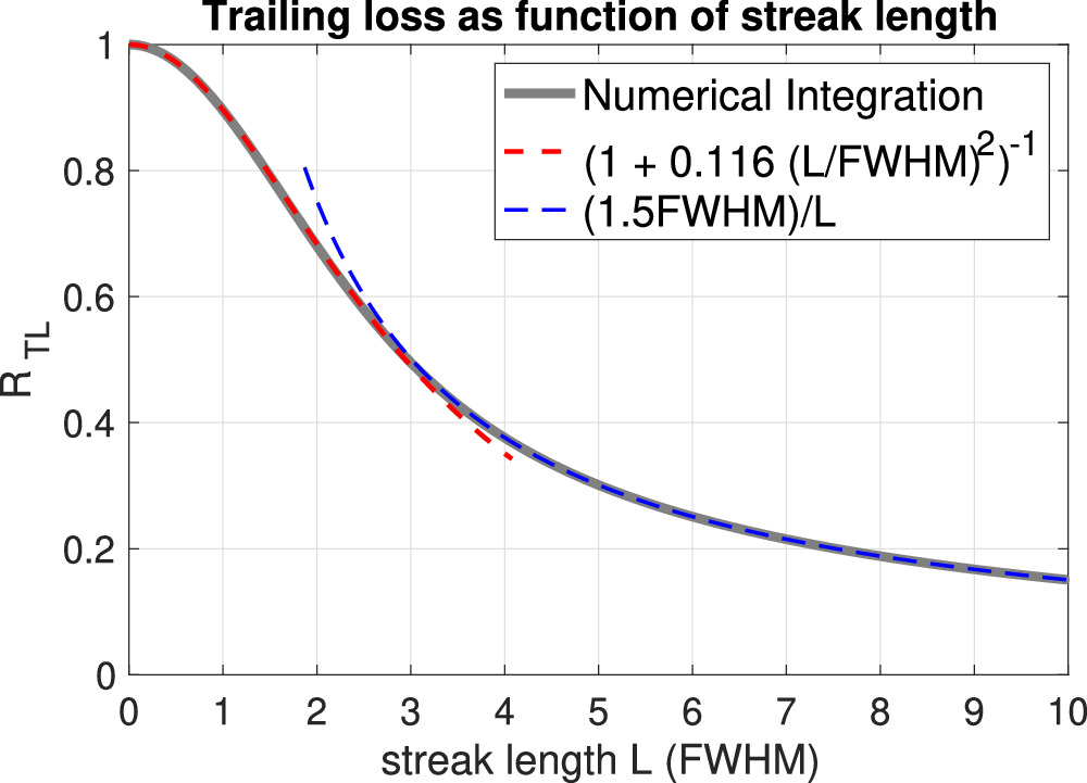
Figure 1. Detection sensitivity with trailing loss as function of the streak length measured in FWHM of PSF. The blue (red) dashed curve represents an approximation for streak length L > 3 FWHM (L < 3 FWHM).
Download figure:
Standard image High-resolution imageIt is useful to introduce a scale for rate of motion as FWHM/τ2, corresponding to a streak length of the PSF's FWHM for exposure time Δt = τ2. If the rate range of interest is much less than FWHM/τ2, we then can easily choose an exposure time Δt to be larger than τ2 for pixel noise to be background noise limited and simultaneously having very little trailing loss. This is the typically the case for using a CMOS camera to observe NEOs because typical CMOS cameras have only 1–2 e read noise when operating in rolling shutter mode (for example, see https://www.photometrics.com/products/prime-family/prime95b). For Pomona College 40 inch telescope at TMF, the τ2 is less than 0.3s. Assuming PSF FWHM is 2 as, FWHM/τ2 ∼ 6.7as s−1 is much higher than typical NEO's sky rate.
To optimize the sensitivity, we include the trailing loss and read noise factor together to define a detection sensitivity S(v, Δt) as

Figure 2 displays contours of constant values of S(v, Δt) as a function of Δt and v in units of Δt/τ2 and FWHM/τ2 respectively. For a given rate of motion range, there is an optimal exposure time marked by the red dashed line. When the rate of motion < FWHM/τ2, we have have a pretty good sensitivity of 0.7 with an optimal choice of exposure time Δt/τ2 ∼ 1.5. If rate of motion < 0.3 FWHM/τ2, this can be improved to 0.85. As an example, considering again our telescope at TMF with τ2 = 0.3 s and FWHM = 2 as giving the unit for velocity FWHM / τ2 ∼ 2/0.3 = 6.7(as s−1). If we are interested in NEOs moving as fast as 1as s−1, or 0.15 in units of FWHM/τ2, we have a range of exposure times would achieve better than 0.85 detection sensitivity regarding trailing loss and read noise trade Figure 2. This is consistent with our discussions regarding the regime where the read noise is much lower than the background noise.
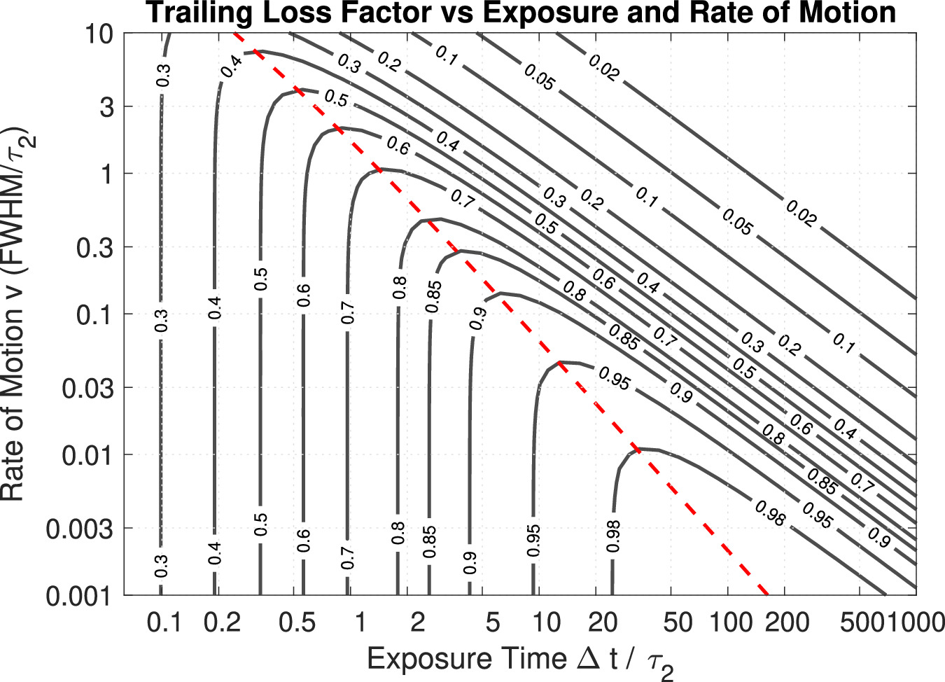
Figure 2. Detection sensitivity as function of rate of motion and exposure time in contours. The red dashed lines represent optimal exposure time for a given velocity.
Download figure:
Standard image High-resolution imageThe discussion above is mainly for observing faint objects, especially for discovering new NEOs, where we have ignored the photon noises from the target itself. In case of observing a bright target, whose photon noise is much higher than the total read noises of all the relevant pixels within a PSF, we in general only need to consider the trailing loss to use an exposure time so that  FWHM.
FWHM.
After choosing an exposure time, the second factor to consider is the total integration time T = Nf Δt, or the number of frames Nf to integrate for the final S/N to be sufficient for detection or achieving certain astrometric accuracy. For example, at SRO, we require a detection threshold of 7.5 for a low false positive rate of 2% per camera field (Zhai et al. 2014). The 40 inch telescope at TMF is mainly used for follow-up observations providing highly accurate astrometry. We have been targeting at better than 100 mas accuracy, which for a PSF size of 2'', this means the S/N would need to be at least 13 in view of uncertainties of centroiding is ∼0.64 FWHM/(S/N) (Zhai et al. 2014). Using results in Appendix A, we have the total S/N
where have introduced total number of photoelectrons  and
and  for the sky background and target, and total dark counts Ndark = TIdark with m0 being the telescope system zero-point (stellar magnitude giving 1 photoelectron/sec), a being the pixel scale, mb
being the background brightness per pixel measured in magnitude, and mt
being the target brightness. In general, using ST, we operate with S(Δt, v) > 0.7 for most of the NEO observations.
for the sky background and target, and total dark counts Ndark = TIdark with m0 being the telescope system zero-point (stellar magnitude giving 1 photoelectron/sec), a being the pixel scale, mb
being the background brightness per pixel measured in magnitude, and mt
being the target brightness. In general, using ST, we operate with S(Δt, v) > 0.7 for most of the NEO observations.
As an example, for SRO1 11 inch telescopes, we use an exposure time of 5 s and a good PSF would have FWHM of 3 as, for our plate scale (∼2.5 pixel). Our 11 inch telescope's zero-point is m0 = 22.1. The dark current is only about 0.5 e s−1 and using the sky magnitude to be 20.5 mag per arcsec square. Putting source brightness mt = 20.5, T = 500s, we get τ2 = 1.62/(0.5 + 1.262 × 10−0.4×(20.5–22.1)) ≈ 0.34 s. We are interested in the velocity range of 0.6 as s−1, or 0.07 in unites of FHWM/τ2 ∼ 9 as s−1. According to Figure 2, the sensitivity S(Δt = 5 s, v = 0.6 as s−1) ≈ 0.9 for using 5 s exposure. The S/N is then
2.2.2. Survey and Follow-up Observation Cadence
We have been experimenting with the SRO1 system to detect new NEOs. We use a 5 s exposure and integrate 100 frames to reach a detection limiting magnitude of about 20.5 for dark nights near new moon (see the example of the last subsection). The SRO1 system has a combined FOV of about 20 sqdeg from the three RASA 11 inch telescopes. On average, we spent about 700 s per pointing, which includes slew time, refocusing time (every 8 pointings), and an extra waiting time for the synchronization of the three telescopes especially the extra 800–900 msec dead time that the ZWO camera has between 5 s frames while QHY cameras do not have this dead time. We scan along the R.A. four consecutive FOVs and then repeat the scan for confirmation. Repeating the scan is operationally inefficient and we are working on a software capability to use the SRO2 system to do follow-up observations upon a detection from SRO1. This triggered follow-up allows SRO1 to scan the sky at a rate two times faster (without the burden of the revisit).
We regularly perform follow-up observations for NEO candidates from the Minor Planet Center's (MPCs) confirmation page (NEOCP, https://www.minorplanetcenter.net/iau/NEO/toconfirm_tabular.html) using the system at the TMF. Because the telescope is sufficiently large, the frame is dominated by sky noise, i.e., τ2 ∼ 0.3 s is small relative to Δt, which we typically use 1, 2, and 3 s exposures and integrate. We usually integrate 300 or 600 frames depending on the brightness and rate of the target.
The 14 inch telescope system SRO2 performs follow-up observations for candidates with large uncertainties in their ephemerides. These candidates are not suitable for the TMF 40 inch telescope to follow due to the small FOV. For NEO candidates from SRO1, we use also 5 s exposure and a 100 frame integration. Our SRO1 system uses S/N threshold of 7.5 to survey NEOs. The larger collecting area of 14 inch (versus 11 inch) and better imaging quality gives us an improvement factor of about 1.6 in S/N, thus SRO2 can reliably confirm the candidates with an S/N of 1.6 × 7.5 = 12 unless they are false detections. 8 This telescope has been also used to confirm objects from the Zwicky Transient Facility (Bellm et al. 2019) and NEO candidates from the NEOCP. We are developing software to fully automate the operation of SRO2 to schedule and perform follow-up observations, as well as processing and submitting the data.
2.2.3. Calibration
For calibration, we generate a mean dark frame, a flat field response, and a list of bad pixels. The mean dark frame is estimated by averaging multiple dark frames taken with the same exposure time as the science data. The flat field response, which physically is the product of the relative pixel quantum efficiency and optical throughput, can be measured by observing the twilight sky. The flat field response can be computed by taking an average over multiple measurements and then normalized so that the mean response over the whole field is 1. See Appendix C for details. We generate a list of bad pixels by applying a noise level upper limit threshold, a dark level upper limit threshold, and a lower limit threshold for flat field response.
2.3. Data Processing
The framework and procedural stages of data processing have been outlined in Zhai et al. (2014). For follow-up observation data processing, Zhai et al. (2018) provides a thorough description of how to generate astrometry for observing known NEOs. Here we give an overview of the data processing, highlight how ST identifies targets, and detail in generating highly accurate astrometry by correcting the DCR effect of the atmosphere as well as accounting for accurate timing when stacking up frames.
2.3.1. An Overview of Synthetic Tracking Data Processing
In the contrast to conventional asteroid detection data processing (Rabinowitz 1991; Stokes et al. 2000; Denneau et al. 2013), ST works on a set of short-exposure images, which we call a "datacube" because of the extra time dimension in addition to the camera frame's row and column dimension. The goal of data processing is to (1) identify the stars in the field and find an astrometric solution to map sky and pixel coordinates; (2) detect significant signals (search mode) or identify target (follow-up); (3) estimate astrometry and photometry for the detected objects or follow-up target.
The data processing consists of three major steps:
- 1.Preprocessing, where we apply calibration data, remove cosmic ray events, and re-register frames to get data ready;
- 2.Star field processing, where we estimate sky background, identify stars in the field, and match stars against a catalog;
- 3.Target processing, where we identify the target and estimate its location, rate of motion, and photometry.
Preprocessing is instrument dependent and generally requires subtracting a mean dark frame of the same exposure time from each frame and then dividing each frame by a flat field response to account for the throughput and QE variation over the field (see Section 2.2.3). While a well-tracking system may not need re-registration, a re-registration is needed for our systems, which could drift more than 10'' during the course of an integration. Re-registration can be done by estimating offsets between frames by estimating positions of one or a few bright stars in each frame or cross-correlating Fourier transforms of each frame. We then remove the cosmic ray events and bad pixel signals by setting the values at these pixels to a background value. Cosmic ray events are identified as signal spikes above random noise level localized in both temporal and spatial dimension.
Star field processing first detects and locates stars in the field by co-adding all the frames with stars well-aligned after the frame re-registration. A planar triangle matching algorithm (Padgett et al. 1997) identifies stars in the field by matching similar triangles formed by triplets of stars at the vertices from both the field and the catalog, where the shapes of triangles are determined by the relative distances between the stars. 9 We use an approximate location of the field, pixel scale, and the size of the FOV to look up the Gaia Data Release 2 (DR2) (Gaia Collaboration et al. 2018) for star identification. This process starts with a small subset of the brightest stars in the field. A pair of correctly matched triangles in the field and catalog gives an affine transformation between the pixel and sky coordinates, which would transform other stars in the field to sky positions close to their catalog positions. To validate a star matching, a large percentage of stars in the field should be matched with the catalog, allowing us to solve for the mapping (the astrometric solution) between the pixel coordinate and the position in the plane of the sky as an affine transformation, and thus the R.A. and decl. Because of non-ideal optics, we often need to go beyond the affine transformation to use two-dimensional lower order polynomials to model the field distortions for more accurate astrometric solutions (see Zhai et al. 2018 for details). For our TMF system with only a FOV of 6', an affine transformation is sufficient for 10 mas accuracy. A 3rd order polynomial is needed to achieve 5 mas accuracy. For SRO1 and SRO2, a 3rd order polynomial is sufficient for achieving 50 mas astrometric solution.
Target processing encompasses identifying a specific follow-up target or searching for new objects. In general, we first removed star signals to by setting pixels near detected stars to zero assuming we have estimated and subtracted the sky background (Zhai et al. 2014), so that we deal with frames with noises and signals from the target or objects to be detected. For a follow-up target with a known sky rate of motion, we can stack up images to track the target. We also apply a spatial kernel matching the PSF to improve S/N. The target is located by finding the pixel that has the highest S/N in the expected region of the field. Sometimes, the target is too faint or the ephemeris has uncertainties larger than what was estimated, human intervention is needed to help identify the object in the field.
In the NEO search mode or when recovering follow-up targets with large uncertainties in ephemerides, we need to use GPUs to perform shift/add over a grid of velocities covering the rate of interest to detect signals above an S/N threshold, which we use 7.5 to avoid false positives (Zhai et al. 2014). The detected signals are clustered in a 4d space (2d position and 2d velocity) to keep only the position and velocity with the highest S/N. The last step in target processing is a least-squares fitting (moving PSF fitting) using a model PSF to fit the intensities of the moving object in the datacube to refine the positions and velocities of the detected signals (Zhai et al. 2014, 2018).
2.3.2. Search for NEOs Using GPUs
The advantage of ST for NEO search and recovery is the improved sensitivity from avoiding the trailing loss at the price of a large amount of computation for processing the short exposure data cubes. For example, our SRO1 system typically uses a 5 s exposure time and integrates 100 frames. The camera frame size is 61 MPix giving a data cube of size about 12.2 GB stored in raw data as unsigned 16-bit integers. During data processing, the data are stored as 32-bit floating point numbers, which means 24.4 GB of memory. Our velocity range of interest is ±0.63 as s−1 (0.5 pixel s−1 for a pixel scale of 1.26 as) over both R.A. and decl. and we use a 100 × 100 grid to cover this range with a grid spacing of 0.0126 as s−1. This means that our maximum rate error is about ±0.0063 as s−1. For 500 s integration, the maximum streak length along a row or column due to this rate error is about 3.2 as or 2.5 pixels. Since our best PSF has a FWHM of about 2.5 pixels, the trailing loss due to digital tracking error is less than 12% as shown in Figure 1. The amount of computation is 61 × 106 × 100 × 100 × 100 ∼ 6.1 × 10¹³ FLOPS per data cube.
Fortunately, modern GPUs like a Tesla V100 allow us to process data in real-time; a single Tesla V100 with 32 GB memory can perform the search in about 440 s. The performance is not limited by the GPU's processing speed but by the memory bandwidth, especially how to efficiently use the cache memory. We note that the velocity grid spacing is determined so that the rate error due to discretization only causes a streak (in post-processing) of no more than 1 PSF per integration. A typical velocity grid spacing is then 2 PSF per integration time. For our SRO1 system, the velocity grid spacing is ∼2 × 2.5 pixel/500 sec ≈ 0.01 pixel s−1. The velocity grid is ±50 in both R.A. and decl. giving a range of rate of ±0.63 as s−1.
When we recover a NEO whose ephemeris becomes highly uncertain, we need to search in the neighborhood of the expected location according to the ephemeris and to cover at least a region of the 3σ uncertainty of the ephemeris. The velocity grid to search should cover around the projected rate of motion also covering at least the 3σ uncertainty of the rate. We use SRO2 to do NEOCP recovery. Because 0.63 as s−1 ≈15 deg day−1, for a newly discovered object without follow-up for 1–2 nights, we typically can recover these objects without trouble because typically the position errors are less than 10 deg and rate errors are less than 10 deg day−1. Since SRO2 has a FOV size of 2.6 × 1.7 deg and for recovery, the uncertainties is along the track of the NEO, thus we only need a one-dimension (instead of 2d) search, so the computation load is much less for recovering an object than the general NEO search.
We note that the range of rate for searching a moving object is only limited by the total amount of computation needed. With multiple GPUs, it is possible to search over even larger range of rate to detect for example earth orbiting objects.
2.3.3. Reduced Systematic Astrometric Errors
Gaia's unprecedented accuracy allows us to push NEO astrometry to 10 mas (Zhai et al. 2018). Highly accurate astrometry requires properly handling systematic astrometric errors such as the DCR effect, star confusion, and timing error.
2.3.3.1. Differential Chromatic Refraction (DCR) Effect
Unless observing at the zenith, the light rays detected are bent by the atmosphere due to refraction. Because the index of air refraction depends on the wavelength of light ∼1/λ2 (Ciddor 2002), the atmospheric refraction bend more the blue light than red light. This introduces a systematic error in astrometry, the DCR effect, if the target and reference objects have different spectra. If a narrowband filter is applied, the DCR effect becomes much less because the variation of atmospheric refraction is significantly reduced by limited passband. However, to detect as much photon as possible to improve S/N, we typically use broadband or clear filters.
DCR effects can be modeled using an air refraction model (Ciddor 2002) and the spectra of target and reference objects (Stone 1996). For 10 mas accuracy, we found it sufficient to use a simple empirical model based on color defined as difference of Gaia magnitudes in blue and red passbands (Andrae et al. 2018) as discussed in Appendix B. The DCR correction in R.A. and decl. between reference color Cref = (B − R)ref and target color Ctar = (B − R)tar is expressed as
where θz is the zenith angle, complementary to the elevation angle, ϕz is the parallactic angle between the zenith and celestial pole from the center of the field. In general, we do not have spectral information of NEO candidates from the NEOCP, so we assume a solar spectrum for them assuming they reflect sunlight uniformly across the band as a leading order approximation with Ctar ≈ 0.85 (estimated using Figure 3 in Andrae et al. (2018) assuming an effective temperature of 5800 K for solar spectrum).
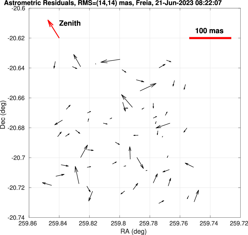
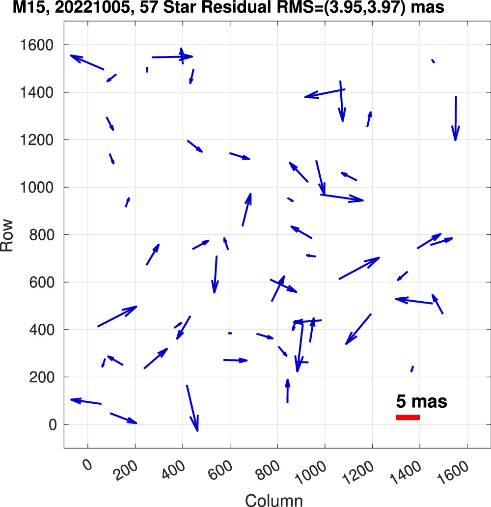
As an example, when we use a clear filter, without any DCR correction, the astrometric residuals for a field observing Feria (76) with a clear filter are displayed in the left plot in Figure 3, where the dominant astrometric residuals are along the direction of zenith from the field. Using Equation (7) to correct the DCR effect for a target with solar spectral type, we significantly reduced the rms of the residuals from more than 40 mas to about 15 mas and the directions of residuals appear random. As a comparison, if we apply a Sloan i-band filter (700–800 nm), the DCR effect becomes smaller than 10 mas because of the limited bandwidth and the less color dependency for longer wavelength because of the dependency of refraction index ∼1/λ2 on wavelength. An additional limitation of bandwidth comes from the falling sensitivity of the Photometrics camera at the longer wavelength making an effectively narrower passband shift to the 700 nm side of the passband. Indeed, without DCR correction, we found that for the same field observing Feria, the rms of astrometric residuals is about 14 mas as shown in Figure 4. Note that the residuals shown in Figure 4 and the right plot in Figure 3 contain significant photon noises. Figure 5 displays residuals observing M15 where only the residuals of bright stars in the field are displayed. Here residuals are not limited by photon noises and we are able to achieve better than 5 mas accuracy.
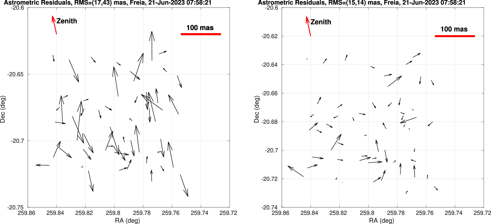
Figure 3. Astrometric solution residuals using a 3rd order polynomial to fit field distortions with the Gaia DR2 catalog to show differential chromatic refraction (DCR) effect with a clear filter. Left plot shows residuals without DCR correct and right plot shows residuals after correcting the DCR effect using a simple quadratic color model.
Download figure:
Standard image High-resolution image
Figure 4. Astrometric residuals of a field observing asteroid Freia (76) using an i-band filter the DCR effects are too small to identify.
Download figure:
Standard image High-resolution image
Figure 5. Astrometric residuals after correcting DCR effects using a clear filter, TMO (654), showing consistency with Gaia DR2 an rms of 5 mas using a third order polynomial field distortion model.
Download figure:
Standard image High-resolution image2.3.3.2. Target Position Estimation and Confusion Elimination
Star confusion is another source of systematic errors for astrometry. We exclude the frames where the NEO gets close to a star whose light could affect the centroiding of the NEO. The centroiding error due to star confusion in units of the FWHM of the PSF is estimated as the gradient of the intensity of the star at the NEO's location relative to the NEO peak intensity divided by its FWHM ∼  . Based on this estimation, we exclude frames that could lead to centroiding errors above a threshold, e.g., 0.01, which should be determined by accuracy requirement assuming this corresponds to a centroiding error ∼0.01 FWHM. The "moving-PSF" fitting is done for frames without confusion. The general cost function for the least-squares fitting of "moving PSF" to the whole data cube
has a weighting function w(x, y, t), which can be set to 0 for frames with confusion. P(x, y) is the PSF function, typically a Gaussian PSF, and  represent the location of the object in frame t, and Nf
is the total number of frames. To minimize the variance of the estimation, the weight can be chosen to be the inverse of the variance of the measured I(x, y, t), including photon shot noise and sky background, dark current and read noise according to the Gauss–Markov theorem (Luenberger 1969). For frames without confusion, we usually choose w = 1 for simplicity because the noise in I(x, y, t) is not the limiting factor of accuracy for most of our targets. For vast majority of objects, the motion can be modeled as linear:
represent the location of the object in frame t, and Nf
is the total number of frames. To minimize the variance of the estimation, the weight can be chosen to be the inverse of the variance of the measured I(x, y, t), including photon shot noise and sky background, dark current and read noise according to the Gauss–Markov theorem (Luenberger 1969). For frames without confusion, we usually choose w = 1 for simplicity because the noise in I(x, y, t) is not the limiting factor of accuracy for most of our targets. For vast majority of objects, the motion can be modeled as linear:
where (xc
, yc
) is the object position at the center of the integration time interval and (vx
, vy
) is the velocity. ( x
(t), y
(t)) are the residual tracking errors (fractions of a pixel) with respect to sidereal after re-registering frames by shifting an integer amount of pixels satisfying
x
(t), y
(t)) are the residual tracking errors (fractions of a pixel) with respect to sidereal after re-registering frames by shifting an integer amount of pixels satisfying  . x,y
(t) can be estimated as the averages of the centroids of reference stars in each frame after frame re-registration (integer shifts of frames). The location (xc
, yc
), velocity (vx
, vy
), and parameters α and I0 are solved simultaneously using a least-squares fitting.
. x,y
(t) can be estimated as the averages of the centroids of reference stars in each frame after frame re-registration (integer shifts of frames). The location (xc
, yc
), velocity (vx
, vy
), and parameters α and I0 are solved simultaneously using a least-squares fitting.
2.3.3.3. Accurate Timing
Accurate timing is crucial for generating precision astrometry. The timestamp for a camera frame in general should correspond to the epoch at the center of the exposure time window for the frame. If possible, hardware timing with a GPS clock is desired because software timestamps from non-real-time operating systems can have errors due to indeterministic runtime behaviors. Hardware timing can be achieved by using a GPS clock to trigger the start of the exposure at a preset time or by letting a GPS clock record the signals generated by a camera upon the completion of a frame. For example, our Photometrics Prime 95B used at TMF can accept a trigger signal from a Meinberg GPS clock to initiate the exposure of frames. Camera reference manual should be referred to interpret timestamps correctly. For example, CMOS cameras have both global shutter and rolling shutter modes and there could be dead time between frames. We usually operate CMOS cameras in the rolling shutter mode for high frame rate and low read noise. Rolling shutter mode delays the exposure time window of each row of the image by a small constant time offset relative to the previous row in the order of readout. It is important to account for this small time delay between the consecutive rows because we usually have the timestamps for reading out the first or last row, but the target is observed at some row in between. This delay is 19.6 usec per row for our Photometrics camera at TMF. A useful test for understanding the details of timing is to use a GPS clock to trigger both the camera and an LED light and examine the recorded frames. Using this test, we found our Photometrics camera has an extra delay of 50 msec for the first frame to start after the trigger signal for the camera.
When excluding frames to avoid star confusion, we need to derive astrometry based on the timestamps of the frames that do not have confusion. For our TMF system, we are confident that our timing accuracy is better than 10 msec, which was confirmed by the small (<0.1 as) astrometric residuals from observing a GPS satellite (C11) relative to the ephemerides from Project Pluto (https://www.projectpluto.com/) and the results from the International Asteroid Warning Network (IAWN) 2019 XS timing campaign (Farnocchia et al. 2022) that we participated in.
3. Results
In this section, we present results from our instrument on the Pomona 40 inch telescope at the TMF and robotic telescopes at the SRO. Our instrument at TMF (654) has consistently produced accurate astrometric measurements and our robotic telescopes at SRO has been able to detect faint NEOs at about mag = 20.5.
3.1. Astrometric Precision using Synthetic Tracking
ST avoids streaked images by having exposures short enough so that the moving object does not streak in individual images, allowing us to achieve NEO astrometry with accuracy similar to stellar astrometry. We have been regularly observing NEOs from the MPC confirmation page since 2021 with a support by the NEOO program targeting NEOs brighter than 22 mag. The left and right plots in Figure 6 respectively display NEO astrometric residuals from subtracting the JPL Horizons ephemerides and the estimated apparent NEO magnitudes from 2021 October to 2023 April after we fixed a timing error.
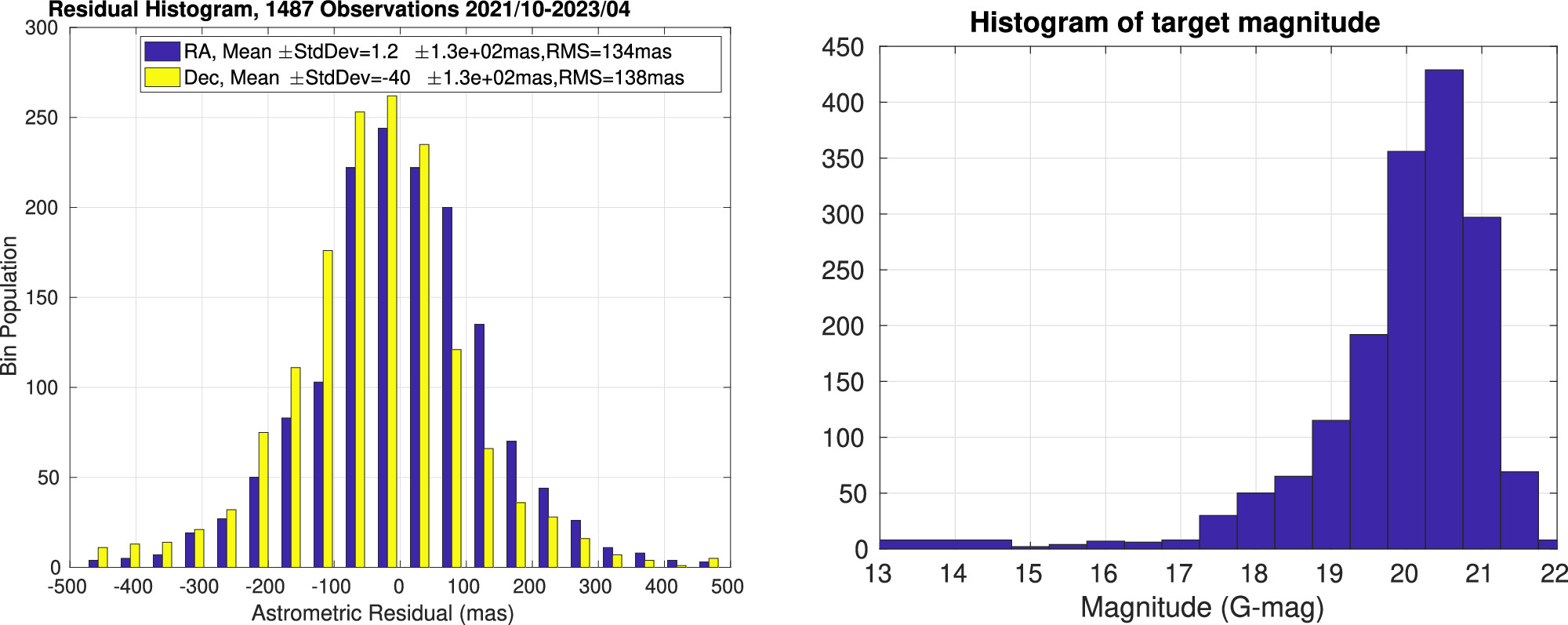
Figure 6. The left plot displays histograms of residuals for R.A. (blue, mean = 1.2 mas, StdDev = 130 mas) and decl. (yellow, mean = −40, Std Dev = 130 mas). The right plot shows the histogram of the target apparent magnitudes.
Download figure:
Standard image High-resolution imageWhile the rms of our residuals are about 130 mas, which is among the best category of NEO astrometry accuracy (Vereš et al. 2017), we believe our accuracy is better than 130 mas because these residuals include the uncertainties of the ephemerides of the NEOs, which are mostly new discoveries with observations covering only a short arc of the orbit. To illustrate this, Figure 7 shows residuals of nine NEOs, where we can clearly see that residuals are biased and the spread of our measurements are much smaller. These biases are consistent with JPL Horizons 3σ uncertainty estimates as shown in Table 2. If instead, we use the standard deviations of our measurements for each target as a measure of astrometric uncertainties to remove the uncertainties in the ephemerides, we get the distribution shown in the left plot in Figure 8. The right plot shows the residuals with the rate of motion. A slight trend of going down is due to the fact that highly moving objects tend to be brighter because of the trailing loss in survey detections as shown in Figure 9.

Figure 7. Examples of uncertainties of NEO ephemerides, the values displayed for R.A. and decl. are means and standard deviations in format mean +/− StdDev.
Download figure:
Standard image High-resolution image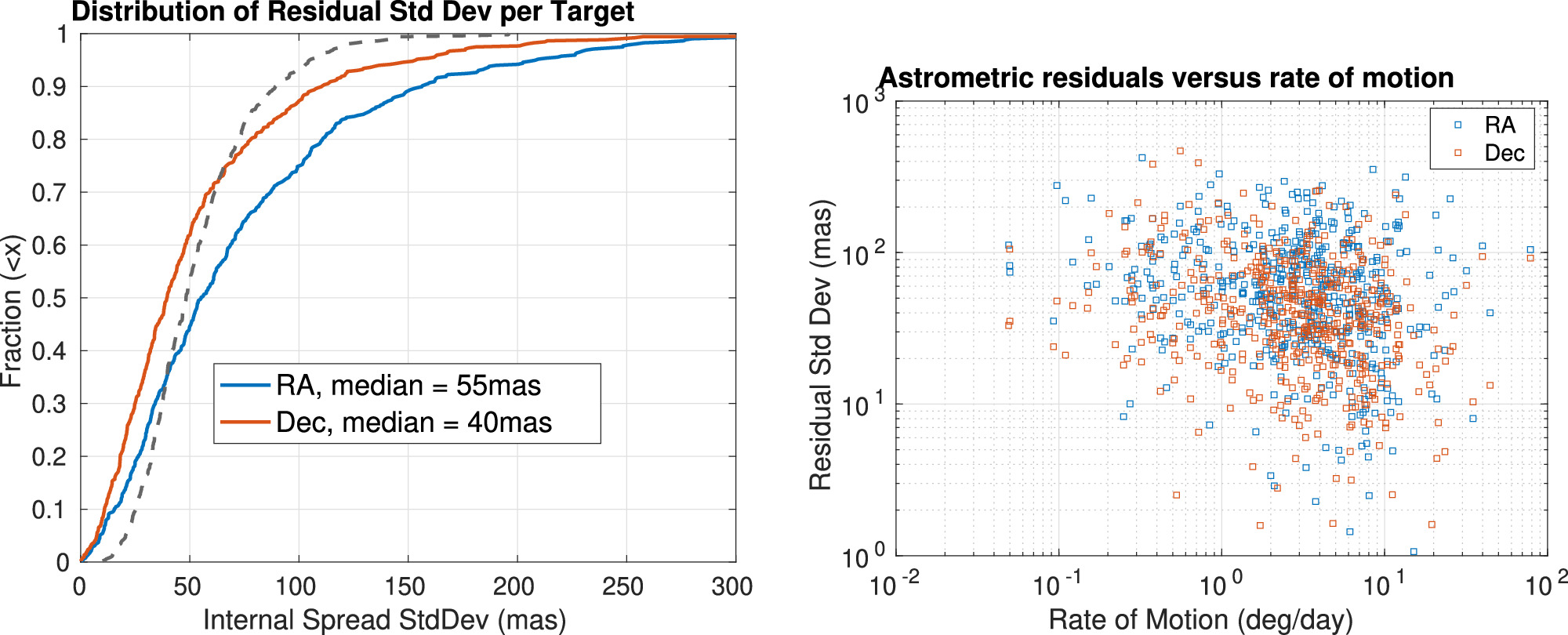
Figure 8. Distribution of standard deviations of the measurements for each target (right), where the black dashed line represent an estimated value of the 1σ uncertainty of the astrometric measurements (left) and the dependency of residual standard deviations vs. rate of motion (right).
Download figure:
Standard image High-resolution image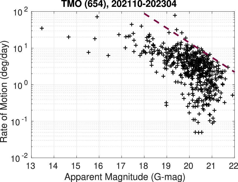
Figure 9. Rate of motion vs. apparent magnitudes of the NEOs from the confirmation page during 2021/10 to 2022/04. The red dashed line represent the relation: rate of motion = (14 deg day−1) ×10−0.4(Apmag−20) showing a deficit of detection of faint fast-moving objects because the brightness limit for detection goes inversely with the rate of motion.
Download figure:
Standard image High-resolution imageTable 2. JPL Horizons NEO Ephemeris Uncertainties and the Residual Biases
| Designation | Epoch | 3σ R.A. (as) | 3σ Decl. (as) | Res R.A. (as) | Res Decl. (as) |
|---|---|---|---|---|---|
| 2021 VF19 | 20211115UT05:00 | 0.532 | 0.533 | 0.13 | 0.015 |
| 2022 AK1 | 20220107UT03:00 | 0.712 | 0.478 | 0.12 | −0.16 |
| 2022 BN | 20220124UT07:30 | 0.517 | 0.535 | −0.24 | 0.23 |
| 2022 BA1 | 20220126UT08:00 | 0.204 | 0.218 | 0.052 | −0.13 |
| 2022 CN | 20220204UT08:30 | 0.469 | 0.455 | −0.069 | −0.44 |
| 2022 CK6 | 20220211UT06:30 | 0.531 | 0.416 | 0.054 | −0.12 |
| 2022 DV2 | 20220227UT07:30 | 0.448 | 0.852 | 0.001 | 0.31 |
| 2022 DU3 | 20220228UT03:30 | 0.168 | 0.223 | 0.040 | 0.13 |
| 2022 ES1 | 20220302UT08:30 | 0.227 | 0.226 | 0.033 | −0.11 |
Download table as: ASCIITypeset image
We note that the bias of about ∼−40 mas in Dec seems to be significant because the mean residual is derived from observations about 500 NEOs with expected random standard error of only  mas. This bias could be related to the fact that we correct the atmospheric DCR effect. If we remove the DCR corrections from our astrometry, we found the bias is close to zeros, as shown in Figure 10.

Figure 10. Histogram of residuals without correcting the differential chromatic atmospheric refraction effect. The R.A. (decl.) residuals have a mean of 5.4 (−8.5) mas and a standard deviation of 130 (130) mas.
Download figure:
Standard image High-resolution imageThe DCR correction is necessary for achieving 10 mas astrometry consistency with the Gaia DR2 catalog as shown in Figures 3 and 5 when using a clear filter. We also found that the DCR correction would give consistent astrometry for bright NEAs like Freia (76). Figure 11 displays residuals of astrometry of our observations on target Freia (76) subtracting the JPL Horizons ephemerides. The squares represent observations using a clear filter. The solid (empty) squares represent results results with (without) DCR corrections for the clear filter. The diamonds are the observations of Freia using a Sloan i-filter, which makes DCR effect significantly smaller that a clear filter because of its smaller bandwidth, the CMOS chip response in this band, and the longer wavelength. The small DCR effect of i-filter is shown by the low residuals of astrometric solution without any DCR correction presented in Figure 4.

Figure 11. An example of DCR correction for a clear filter together with the observation with a Sloan i-filter. Without DCR correction, the R.A. (decl.) residuals for using a clear filter, represented by blue (red) empty squares, have a mean of 19 (122) mas and a standard deviation of 22 (8.7) mas. After applying the DCR correction, the R.A. (decl.) residuals for using a clear filter, represented by blue (red) solid squares, have a mean of 13 (−6.7) mas and a standard deviation of 2.2 (6.9) mas. The R.A. (decl.) residuals for using a Sloan i-filter has a mean of 11 (−0.79) mas and a standard deviation of 1.1 (0.84) mas.
Download figure:
Standard image High-resolution imageThe fact that the DCR correction makes broadband astrometry much closer to an i-band filter with lower astrometric residuals as shown in the right plot in Figure 3 validates our approach of DCR correction. To the first order, we assume solar spectrum for NEOs. However, NEO spectra can deviate from the solar spectrum, so improvements can be made by measuring the color of the NEOs. To our knowledge, vast majority of the NEO observations do not correct the DCR effects, therefore these astrometric measurements are biased due to DCR effects. The DCR effects tend to introduce an overall bias along Dec depending on the average elevations of observations because DCR effects along R.A. can be both positive or negative depending on the sign of hour angles, thus not necessarily introducing an overall bias. If this is the case, the derived ephemerides could be then biased in Dec due to most of the measurements used are not DCR corrected. Measurements with DCR corrections like ours would appear biased along decl. relative to these ephemerides. It would be interesting to further understand this bias by comparing all the observations with and without DCR corrections and the filters applied.
3.2. Robustness Against Star Confusion
Confusion occurs when a NEO moves very close to a star. If tracking the NEO, the stars streak. In case of confusion, the streak of a star would overlap with the tracked NEO. This is an extra burden for operations to avoid confusion, which can be challenging if observing a dense field. ST is robust against this confusion because we take short exposures. In post-processing, we can exclude the frames that have confusion as discussed in Section 2.3.3.2. Figure 12 shows an example to illustrate our approach. The left plot shows the field with the green dashed line marking the track (from upper right to lower left) of NEO 2022UA 21 with an apparent magnitude of 17.3 during our observation. It encounters a 15 mag star, much brighter (about 10 times) than the target. We quantify the confusion by computing the intensity gradient of the confusion star at the target relative to the target intensity gradient (approximately the peak intensity divided by the FWHM) as the measure of the confusion  . For this case, the confusion measure is displayed in the mid plot in Figure 12. The right plot shows all the clean frames stacked up tracking the target. Excluding frames with confusion creates gaps in the star streaks so that the target shows in the gap as a compact object without contamination of photons from the stars. This is particularly useful when the field is crowded, as shown in Figure 13.

Figure 12. Star confusion field (left) and a measure of confusion (right).
Download figure:
Standard image High-resolution image
Figure 13. Star confusion field (left) and a measure of confusion (right).
Download figure:
Standard image High-resolution image3.3. Recovery of Candidates with Highly Uncertain Ephemerides
The ephemerides of fast-moving NEOs tend to develop uncertainties quickly after the initial detection due to the propagation errors from the nonlinearity introduced by the quickly changing observation geometry. Timely follow-up observations are crucial for tracking these fast-moving NEOs. However, it could happen that fast-moving NEOs are discovered without timely follow-up observations due to the unavailability of follow-up facilities, poor weather/day-light conditions for observation, or latency in data processing. Because most of the follow-up facilities do not have large FOVs and the vast majority of the facilities rely on tracking the object to avoid trailing loss, it is quite hard to recover an object that has larger than 1 deg angular uncertainties in the sky position. Fortunately, our SRO2 (U74) system with ST has good capability to recover NEO candidates with relatively large uncertainties because ST does not require accurate knowledge of the rate of motion and our 4.47 sqdeg FOV is capable of searching efficiently a large portion of the sky. To illustrate this capability, Table 3 summarizes four examples of recovery using SRO2, where we show the large uncertainties of the ephemerides derived from the initial discovery in the second column and the last column is the uncertainties after we recover the object. For example, 2021 TZ13 was discovered on 20211010, based on only four observations, the ephemerides are highly uncertain with error 1–5 deg. Our SRO2 recovered this object, which otherwise would have been lost. Other examples of recovery are for 2022 MD3, 2023 BH5, 2023 BE6.
Table 3. NEO that are Recovered Succesfully
| Asteroid | Uncertainty at Recovery | Brightness (mag) | Uncertainty at Next |
|---|---|---|---|
| Designation | SRO2 (U74) | (mag) | Follow-up Observation |
| 2021 TZ13 | 1–5 deg | 19.8–20.0 | 2–6 as |
| 2022 MD3 | 5–15 deg | 19.4–20.0 | 2–5 as |
| 2023 BH5 | 28–35 deg | 19.5–19.8 | 2–9 as |
| 2023 BE6 | 3–9 deg | 19.8–20.1 | 90–150 as |
Download table as: ASCIITypeset image
3.4. Detection Sensitvity
Using ST to survey fast-moving NEOs avoids the trailing loss, and thus reaches detection sensitivity as if we were tracking the targets. This enables small telescopes to observe and detect NEOs using long integrations, which would not be possible if the trailing loss degrades the S/N as we integrate long (see Figure 2 for the degraded sensitivity when Δt increases beyond the optimal exposure time). We have been experimenting with our 11 inch telescope system SRO1 (U68) to survey NEOs with a 5 s exposure time and an integration of 100 frames, giving a limiting magnitude of ∼20.5 for clear dark nights.
Currently, our operation observes each field twice during the same night with about 45 minutes between the visit and revisit. With three telescopes (total 22 sqdeg FOV), we can cover approximately 300 sqdeg per night and the whole sky in about 10 days. Each ST observation gives an estimate of the sky position and rate of motion along R.A. and decl. for the target. We can determine whether two observations at different epochs are for the same object by checking whether the rates of motion from the two observations are consistent with the position changes between the two epochs for a linear motion. If the visit and revisit provide two consistent detections of the same object, we essentially have a tracklet of four observations for the same object, thus the detections are reliable and the data is then reported to the MPC.
At the time when the manuscript was generated (around mid 2023 June), we have discovered 62 new NEOs since 2018. A steady process has been made toward more efficient operation procedures, better imaging quality, and more reliable software as reflected by the number of detections shown in the left chart in Figure 14. We are also working on an automated relay between the survey SRO1 (U68) and the follow-up SRO2 (U74) systems. According to MPC (https://minorplanetcenter.net//iau/lists/YearlyBreakdown.html), the yield of 27 new NEOs in year 2022 from our pilot study over about 90 nights puts SRO1 (U68) at the sixth place in the number of new NEOs discoveries, after Pan-STARRS (F51, F52), CSS (G96, V00, 703, I52), ATLAS (M22, T08, T05, W68), MAP (W94, W95), and GINOP-KHK (K88).
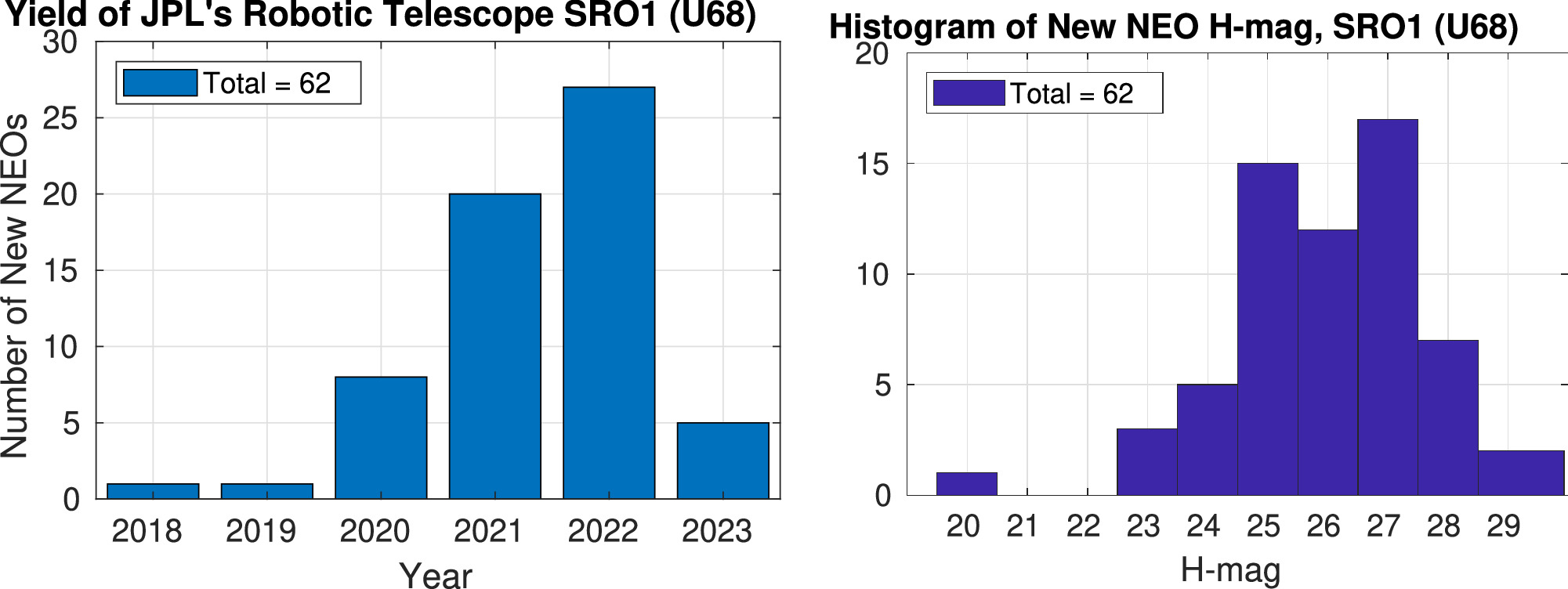
Figure 14. Histogram of discoveries by JPL's robotic telescope at SRO (U68).
Download figure:
Standard image High-resolution imageFigure 15 shows the rate of motion and the apparent magnitudes for all the observations (black plus sign) that we reported to MPC. The plus signs surrounded by red boxes are our new discoveries. These 11 inch telescopes can observe NEOs beyond 20.5 mag, regardless of the rate of motion, as we estimated in Section 2.2.1. This is different from what was shown in Figure 9, where we clearly see a deficit beyond the red dashed line represented by the relation: rate of motion = (14 deg day−1) × 10−0.4(mag−20), inverse with the brightness), showing clearly major survey facilities suffer trailing loss with limiting brightness (or detection magnitude) inversely proportional to the rate of motion as shown in Figure 1. Figure 15 demonstrates the efficacy of ST in searching faint fast-moving NEOs complimentary to the major survey facilities.
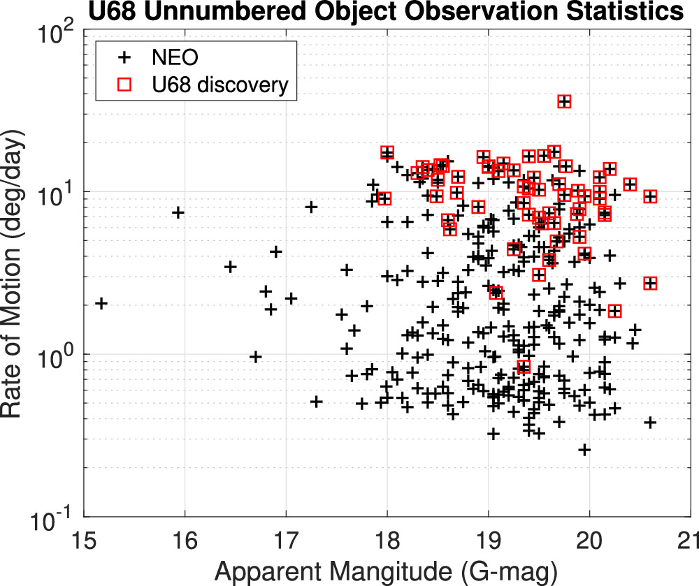
Figure 15. The rate of motion and apparent magnitude plot for observations from JPL's robotic telescope SRO1 (U68).
Download figure:
Standard image High-resolution imageFigure 16 shows the detection of a fast-moving object, 2022 UA28, which represents the current frontier of faint fast-moving detection. The object was moving at a rate of 11 deg day−1, (−7.6, 8.1) deg day−1 along (R.A. decl.) with apparent magnitude of 20.5 mag. If using an exposure time of 30 s, the streak length would be 138. Assuming 2 as FWHM for PSF, the trailing loss would be a factor ∼13.8/(1.5 ∗ 2)4.6, so more than 1.5 stellar magnitude fainter. (For Pan-STARRS, this would be even more as the integration time is 45 s and the PSF is more compact than 2 as.) We detected this object as an S/N about 8.3 enabled by ST.
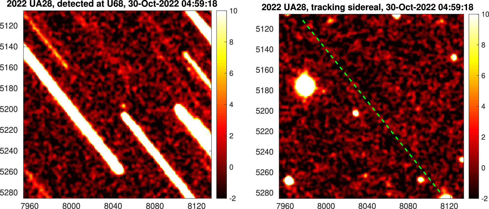
Figure 16. An example of NEO (2022 UA28) discovered by JPL's robotic telescope at SRO1 (U68) Left image shows integration tracking 2022 UA28 (at the center) and right image is the integration tracking sidereal with the NEO track marked as the green dashed line, where the trailing loss makes NEO signal buried in noises.
Download figure:
Standard image High-resolution image4. Summary, Discussions, and Future Works
In summary, ST is effective for observing fast-moving NEOs by avoiding trailing loss to gain detection sensitivity and astrometric accuracy. As the field is moving forward quickly, more small telescopes working with CMOS cameras are used for NEO observations. These systems are ideal for adopting ST as we have demonstrated with our robotic telescope systems SRO1 (U68) and SRO2 (U74) at SRO. Even with the economic COTS hardware, ST is pushing the current state-of-the-art for surveying fast-moving NEOs to rate faster than (0.5 as s−1) and magnitude beyond 20.5. We recently installed a new system at the Lowell Observatory to have a cluster of four 14 inch telescopes (U97), which can be operated in two modes, collapsed mode (all the telescopes pointing at the same FOV) and the splayed mode where the telescopes point at adjacent fields. This is a modern approach for flexibility of using ST to search either deep or a large field.
In the past few years starting from the year 2000, the contributions to the total detection from other facilities than the major survey facilities like Pan-STARRS and CSS have been steadily increasing. One driving factor is the usage of CMOS with small telescopes and ST. One star player is MAP observatory (W94, W95), ranked fourth place among the surveys, discovered 69 new NEOs in 2022 using ST. We hope this article will help the community use ST to speed up the process of inventorying all the NEOs relevant to planetary defense. Accurate astrometry provides more accurate future orbital paths for close Earth approaches and more reliable estimation of probabilities of impacting Earth. Another application of accurate ground-based astrometry is in the optical navigation of future spacecraft that carry laser communication devices, whose downlink may be used to determine the plane of sky position.
Acknowledgments
The authors would like to thank Heath Rhoades at the Table Mountain Facility of JPL, Tony Grigsby, and Hardy Richardson at the Pomona College for supporting the instrumentation, and Paul Chodas at JPL for technical advices on using the JPL Horizon System. We thank all the students at the Pomona College who involved in carrying our the NEO observations using the TMF system. We thank Peter Vereš at the Minor Planet Center for constantly giving us feedback on our observational data, Bill Gray at Project Pluto and Davide Farnocchia of JPL for helping us improve timing. We appreciate the anonymous reviewer's thorough review and helpful comments for improving the manuscript. This work is supported by NASA's ROSES YORPD program and JPL's internal research fund. This work has made use of data from the European Space Agency (ESA) mission Gaia (https://www.cosmos.esa.int/gaia), processed by the Gaia Data Processing and Analysis Consortium (DPAC, https://www.cosmos.esa.int/web/gaia/dpac/consortium). Funding for the DPAC has been provided by national institutions, in particular the institutions participating in the Gaia Multilateral Agreement. The work described here was carried out at the Jet Propulsion Laboratory, California Institute of Technology, under a contract with the National Aeronautics and Space Administration. ©2024. All rights reserved. Government sponsorship acknowledged.
Appendix A: Detection Signal-to-Noise Ratio for Guassian PSF and Trailing Loss
In this appendix, we compute the detection S/N for a Gaussian PSF
normalized so that ∑x,y Pg (x, y) = 1. We also assume that the PSF is critically sampled. The total noise in a pixel per frame σn is

where Δt is the exposure time, Idark is the dark current, and Ibg is the background flux. For simplicity, and as a good approximation, we consider only a uniform background, uniform dark current, and uniform read noise over all the pixels. For a point source (e.g., a star) with flux of Is, the counts detected during one exposure are Is Pg (x, y)Δt. A matched filter with kernel Pg (x, y) gives the highest signal-to-noise ratio (S/N) for detecting the starlight. We calculate the signal as

and the variance of noise as

where we have assumed that the noises of pixels are not correlated. Computing
single frame S/N is
The full-width-at-half-maximum (FWHM) is commonly used to specify the size of a PSF. FWHM of a Gaussian PSF is given by

The S/N for a single frame can be written as
which means that a Gaussian PSF has the same detection sensitivity as a top-hat square PSF with size ∼1.5 × FWHM.
We now estimate the trailing loss due to motion of the source such as a NEO. For a streaked image with streak length L, we have the image intensity

Ideally, we should use a filter matching I(x, y) to detect a moving object. However, since we do not know the motion in advance, we only use a kernel matching Pg (x, y) for detection. The convolved signal with a kernel centered at (xc , yc ) that matches Pg (x, y) is given then
Computing
we get
For the detection of the signal, we only need to consider the maximum of the signal over (xc
, yc
). Therefore, we set xc
= 0. In viewing of that the integral over  reaches maximum when yc
= L/2 by symmetry, i.e., putting the kernel at the center of the streak. We thus have the maximum signal
reaches maximum when yc
= L/2 by symmetry, i.e., putting the kernel at the center of the streak. We thus have the maximum signal
where have changed variable from  to
to  and used symmetry of the integrand between
  and
and  . Therefore,
where we have introduced a reduction function RTL due to trailing loss

For small s, the following expansion is useful
For large s, it is useful to express RTL(s) in terms of the Gaussian error function as
Figure 17 plots the RTL as function of s.
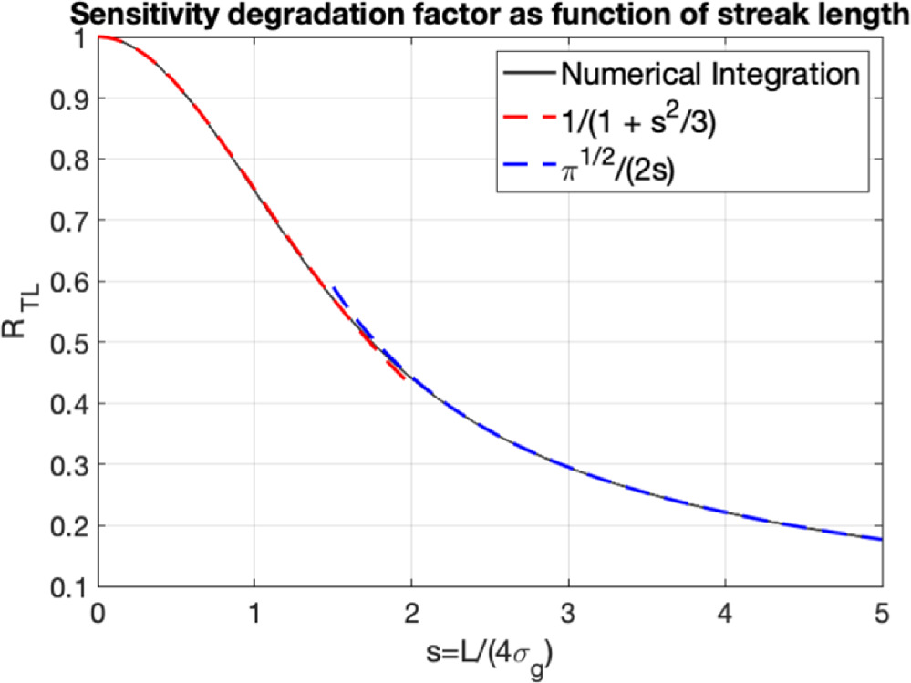
Figure 17. Trailing loss sensitivity factor as function of streak length.
Download figure:
Standard image High-resolution imageLooking at the expansion and the curve, we have the following approximation
We can now estimate the trailing loss for a streak length equals the FWHM of the PSF, for which s ≈ 0.6 upon using Equation (A7). The loss is roughly 0.62/3 ≈ 11%, so in general keeping the streak length less than the FWHM of the PSF is quite good already. But, we can further determine the preferred exposure time by maximizing the sensitivity for a fixed integration time T = Nf Δt, where Nf is the number of frames. The total S/N for integrating Nf frames is
Inserting Equation (A2) gives
It is convenient to introduce timescale, τ1 for the object to move 4σg ,

Using Equation (2), the dependency of S/N on Δt can be expressed as
Taking derivative with respect to Δt gives the optimal exposure time Δt that maximizes S/N to satisfy the following equation
which can be simplified as
Using the standard root formula for a cubic equation, we have the solution
In the region where we are dominated by the sky background noise, τ2/τ1 ≪ 1, we have the following approximated formula
Figure 18 shows the optimal exposure time as function of the ratio of the two timescales of τ2 and τ1. The ratio τ2/τ1, given by
has the physical meaning of the ratio of variances due to read noise and background level integrated over the time of τ1, which is the time for the object to move 4σg ≈ 1.7 FWHM.

Figure 18. Optimal exposure time as function of the ratio of timescales of τ2 and τ1.
Download figure:
Standard image High-resolution imageFor applying ST, we typically are in the region when τ2/τ1 < 1 and the streak length is not too large compared with the PSF size. Since we usually use the FWHM to measure the size of PSF and the streak length instead of using 4σg , we summarize our results for convenient use as follows.
For short streak length L < 3 FWHM, an approximate reduction factor of S/N is given by
For long streak length L > 3 FWHM, sensitivity reduction factor of S/N is given by
Appendix B: Differential Chromatic Refraction Correction
Because the atmosphere refracts star lights, stars appears as closer to the zenith. The refraction index of the atmosphere depends on the wavelength as ∼1/λ2, thus the refraction effect of blue stars is larger than that of red stars. For astrometry, we only need to estimate the position of the target relative to reference stars. If the target and the reference stars all had the same color, the atmospheric refraction effect would be then canceled up to the field dependent geometric effect, which can be modeled by the field distortion. However, the target and the reference stars are, in general, of different stellar types, we therefore need to correct the DCR effect. This effect can be mitigated by applying a narrow band filter, but this also reduces the amount of photons, which may introduce too much photon noise. Another way is to limit the stellar type ensure they are close the type of the target, this however will significantly limit the amount of stars; and thus may lead to poor astrometric solutions. Fortunately, the DCR effect can be modeled using the air refraction index (Stone 1996) and the spectra of objects. For example, Magnier et al. (2020) used a linear color model to correct DCR effects for Pan-STARRS1 astrometry calibration. Here we found, for 10 mas accuracy, this refraction effect can be modeled with a simple quadratic color model:

where θz is the zenith angle, complementary to the elevation angle, ϕz is the parallactic angle between the zenith and the celestrial pole from the center of field, and C ≡ B − R is the difference of Gaia's blue-pass filter magnitude B and red-pass filter magnitude R (Andrae et al. 2018). a and b can be estimated according a dense field with sufficient stellar spectral diversity. Model (B1) is the base for Equation (7), which gives the DCR correction accounts for the spectral difference between the reference and target objects in terms of reference star color Cref and target color Ctar. Note that the DCR effect depends on the passband used for observations and this dependency is captured by parameters a and b. To maximize photon usage for sensitivity, we use the full band of the CMOS ("clear filter") by default. We observed the Freia (76) asteroid using a clear filter and also a Sloan i-band filter. Without and with DCR correction, we have residuals as displayed in the left plot in Figure 3 where we can see errors shown as a two-dimensional vector tend to align with the direction pointing to the zenith. Displaying the component along the zenith direction (altitude) and the direction perpendicular to the zenith direction, which we call the azimuth direction, we found that these errors have a systematic dependency (dominantly linear) with the star colors Cref = (B − R)ref. This supports the model (B1). A quadratic fit to this kind of curve allows us to determine coefficients a and b empirically. For example, for our "clear band," a ≈−168 mas and b ≈ 20 mas. In contrast to the clear filter, the residuals shown in Figure 4 for the i-band filter is hard to identify and the color dependency is hard to see suggesting that a and b for i-band is smaller than 10 mas. We also display the astrometric residuals with i-band filter and the DCR effects are much smaller buried in the random noises as shown in the right plot in Figure 19.

Figure 19. Astrometric errors due to the DCR effect is approximately a linear function of color in left plot for a clear filter; the dependency is not significant for i-band filter as shown in the right plot.
Download figure:
Standard image High-resolution imageAppendix C: Flat Field Calibration
The twilight flat field calibration can be performed in two ways. One setup is to take the measurements when the twilight light is much stronger than any stars in the field so that photons from stars in the field can be ignored relative to the sky background. To avoid saturation, we typically use a very short exposure (no more than 0.1s) to keep the pixel light level for the twilight sky at about half full-well counts. Turning off the tracking to let stars drift in the field helps because the trailing loss further reduces the star lights relative to the twilight sky background. We usually take hundreds of frames and it is straight forward to take an average over these frames and perform a normalization to yield a flat field response. However, this approach requires the experiment to be carried out in a very limited time window during twilight.
In case of missing the desired twilight time window, an alternative approach for flat field response calibration can be employed. This approach involves activating sidereal tracking and deliberately shifting the pointing to capture multiple sky background images with stars at different pixel locations in the field. This diversification guarantees that each pixel has multiple opportunities to exclusively capture the sky background free of star-generated photons. Subsequently, the data is processed by first eliminating pixel data where star signals are detected. After scaling the sky background of each sky image to the same level, an average can be computed for each pixel across the image set, exclusively considering instances when the pixel registers the sky background without any star signals. The data processing is slightly more involved, but we gain the flexibility of when to take the data. This approach works even when the sky background is not high, where a longer integration can be implemented as needed.
Footnotes
- 6
- 7
NEOs with higher rate can often be detected even with the trailing loss because they are close to the Earth with sufficient brightness.
- 8
We use a threshold of 7.5 corresponding to an event with probabilty of erfc
 assuming a normal distribution, which gives a false positive rate of about 2% considering 100 × 100 trial velocities together with the 60 Mpixel frame size. If confirmed, the chance for this detection being a false detection would be pratically zero because we require the rates of motion of the two detections to be consistent and the position changes between the two detections to be consitent with the rate of motion.
 - 9
We prototyped data processing in Matlab and adopted tri_match_lsq.m from http://weizmann.ac.il/home/eofek/matlab/ for star matching. We had to fix bugs to make it working. We then rewrote everything in C++.
