

Abstract
The demand for traceable hydrophone calibrations at low frequencies in support of ocean monitoring applications requires primary standard methods that are able to realise the acoustic pascal. In this paper, a new method for primary calibration of hydrophones is described based on the use of a calculable pistonphone to cover frequencies from 0.5 Hz to 250 Hz. The design consists of a pre-stressed piezoelectric stack driving a piston to create a varying pressure in an air-filled enclosed cavity, the displacement (and so the volume velocity) of the piston being measured by a laser interferometer. The dimensions of the front cavity were designed to allow the calibration of reference hydrophones, but it may also be used to calibrate microphones. Examples of calibration results for several sensors are presented alongside an uncertainty budget for hydrophone calibration with expanded uncertainties ranging from 0.45 dB at 0.5 Hz to 0.30 dB at 20 Hz, and to 0.35 at 250 Hz (expressed for a coverage factor of k = 2). The metrological performance is demonstrated by comparisons with results for other calibration methods and an independent implementation of primary calibration methods at other institutes.
Export citation and abstract BibTeX RIS

Original content from this work may be used under the terms of the Creative Commons Attribution 4.0 license. Any further distribution of this work must maintain attribution to the author(s) and the title of the work, journal citation and DOI.
1. Introduction
There are a wide range of applications in ocean acoustics which require measurement at very low acoustic frequencies (below 100 Hz). These include acoustic surveying for oil and gas exploration, monitoring of tsunamis using ocean bottom sensing networks, naval defence applications, and monitoring for nuclear testing by the international monitoring system of the comprehensive test ban treaty [1, 2]. Low frequency measurements are required for the study of sounds made by natural sources such as ice calving, baleen whales and earthquakes [3–5]. Noise pollution from anthropogenic sources is increasingly recognised as an environmental concern and is now the subject of regulation [6, 7] with the sources of greatest concern being at low frequencies where the propagation of sound leads to large environmental footprints and where sources are sometimes of high acoustic energy. Such sources range from offshore construction [8] to explosive decommissioning for disposal of unexploded ordnance [9], and from operational noise of marine renewable energy installations [10] to airgun arrays used in oil and gas exploration [11]. In addition, oceanographic studies into trends in anthropogenic noise and large scale ocean processes require measurements using hydrophones in the frequency range below 100 Hz [1, 2, 12, 13].
Where absolute measurements are needed, traceable hydrophone calibrations are required, which in turn require primary standard methods that are able to realise the acoustic pascal. Ideally, a number of methods would be used to enable comparison between results obtained by independent methods based on different physical principles, thereby achieving a higher degree of confidence in the realisation. In underwater acoustics, a number of primary methods have been developed, and some have been standardised in international standards [14]. These include the method of coupler reciprocity in which three transducers are inserted into a fluid-filled coupler and calibrations are made traceable to electrical standards with a knowledge of the acoustical compliance of the coupler [15, 16]. Other methods include the hydrostatic excitation method where the hydrostatic pressure is very slowly varied in a coupler by raising and lowering a secondary chamber [17, 18], the vibrating column method and the standing-wave tube [19–21].
In this paper, a new method for primary calibration of hydrophones is described based on the use of a calculable pistonphone [22] to cover frequencies from 0.5 Hz to 250 Hz. A piston driven by a prestressed piezoelectric stack creates a varying pressure in an enclosed cavity. The displacement (and so the volume velocity) of the piston are measured by an optical interferometer. The dimensions of the front cavity were designed to allow the calibration of reference hydrophones, but it may also be used to calibrate microphones. The method of the calculable pistonphone has been used in air acoustics as an absolute method for calibration of microphones, the volume velocity of the piston often being measured by use of optical methods [23, 24]. The work described here builds upon the pioneering work that established the first laser pistonphone [25]. When applied to hydrophone calibration, the method exploits the fact that the sensitivity of an acoustically hard hydrophone is the same in air as in water at low frequencies. Previous reports [23–25] of the use of pistonphones for hydrophone calibration have mostly been for a relative calibration method, though some absolute calibrations have also been reported. The National Physical Laboratory (NPL) implementation of the calculable pistonphone now demonstrates the feasibility of this method for calibrating hydrophones in air in the frequency range from 0.5 Hz to 250 Hz. The method has been validated by comparison to independent methods at other NMIs using microphones as the transfer standard.
This paper describes the operation of the calculable pistonphone and shows results for the calibration of a hydrophone and a microphone with comparison to other independent methods for validation. This is followed by a discussion of the limitations and challenges of the method, an uncertainty assessment, and then a discussion of the validation is provided.
2. Calibration by calculable pistonphone
2.1. Basis of method
In brief, the calibration principle of a calculable pistonphone is that the sound pressure in a sealed cavity driven by a piston can be determined when the displacement of the piston is known. In this pistonphone, the dynamic displacement of the piston is measured using optical interferometry and enables determination of the volume velocity, assuming a rigid piston with known surface area.
The resulting sound pressure p due to this volume velocity is governed by the acoustical impedance  of the coupler, which is effectively a pure compliance. Strictly the acoustical transfer impedance should be considered, but in the low frequency range of interest, a spatially uniform sound pressure can be assumed, such that:

where  is the volume change introduced by the piston driven at a frequency
  , and
, and
where  is the total volume,
  the static pressure and
  is the ratio of specific heats for air, when the acoustic impedance is a pure compliance.
The assumption of spatially uniform sound pressure effectively means that the acoustic wavelength must be considerably larger than any dimension of the cavity. The precise relationship depends on the measurement uncertainty that can be accepted, but as a rule of thumb, the upper frequency limit corresponds to a wavelength approximately twenty times the largest dimension of the cavity.
The appearance of the ratio of specific heats in the formulae above derives from the assumption that the acoustic process is adiabatic. However, as the frequency reduces, there is a transition towards isothermal behaviour, and a correction to the calculated sound pressure is necessary to account for the influence of heat conduction. A correction based on the model given in IEC 61 094–2 [26] is calculated for the specific geometry of the pistonphone.
The sensor to be calibrated is then exposed to this known sound pressure, and its output voltage  is measured. The sensitivity modulus, MH is then calculated from:
2.2. NPL implementation
2.2.1. Pistonphone body.
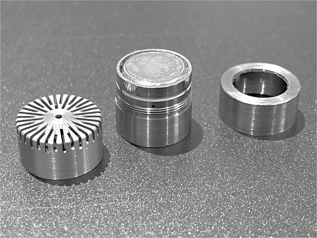
The NPL pistonphone is a metal structure with a cylindrical chamber that sits above a laser interferometer. A cross section of the chamber is shown in shown in figure 1. The hydrophone is inserted into the chamber through a lid at the top forming the upper boundary. Alternative lids can be used to allow the mounting of different devices or in some cases extended lids can be employed which shorten the length and reduce the volume of the chamber, thereby increasing the sound pressure the hydrophone is exposed to and increasing the upper frequency that is measurable. The piston face forms the bottom boundary of the chamber. Both the chamber lids and piston are sealed onto the wall of the chamber with dual O-rings.
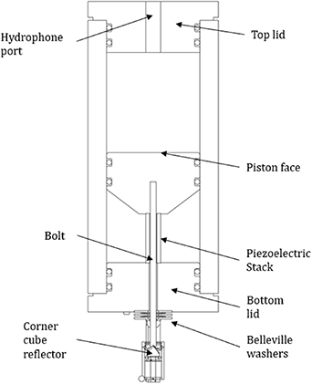
Figure 1. Cross-section diagram of the NPL pistonphone body.
Download figure:
Standard image High-resolution imageA bolt connected to the piston, goes through the piezoelectric stack and protrudes through the bottom lid of the structure. A corner cube reflector is attached to the bottom of the bolt which allows the displacement of the piston to be measured with the interferometer.
The pistonphone chamber has a nominal inner height of 86 mm and nominal diameter of 75 mm when using a thin lid as shown in figure 1. The entire setup is situated on an optical table designed for minimizing interference from vibration and is situated in a temperature-controlled room. The atmospheric pressure is not controlled but it is measured at the time of a calibration and accounted for in the calculation of the sound pressure.
The pistonphone is fitted with a valve connecting the chamber with the outer atmosphere (see figure 4). It provides the means to test the chamber for leaks. Any leakage occurring through the O-rings or seals on the hydrophone or microphone would result in the sound pressure being lower than determined from the interferometer, resulting in an apparent roll-off in the frequency response of the measured sensitivity of the device.
In order to examine the pressure variation received by the hydrophone inside the pistonphone chamber, a numerical simulation with PAFEC, a commercial finite/boundary element software [27] was applied to calculate the pressure distribution. A 2D model was applied since the problem is axisymmetric (see figure 2) around the centreline of the hydrophone.
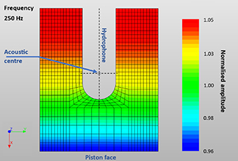
Figure 2. The variation of sound pressure in pascals as a function of radius (y in the plot) and length (x in the plot) at 250 Hz with a uniform velocity drive at 1 m s−1 from the right end in the length direction.
Download figure:
Standard image High-resolution imageThe mesh was selected such that the largest dimension of the largest finite elements was less than one third of the wavelength at the highest frequency of 250 Hz. Figure 2 shows the variation of sound pressure as a function of radius (denoted as y in the plot) and length (denoted as x in the plot) at 250 Hz with a uniform velocity drive at 1 ms−1 from the right end in the length direction. It can be seen that the difference between the extremes of the minimum and maximum pressures is small at about 10%, and that the variation in the region of the hydrophone element is much smaller still.
The pressure received by the hydrophone was averaged over the cylindrical element at a radius 10.5 mm over a length of 17 mm around its acoustic centre. Figure 3 shows the relative pressure (the average pressure over the hydrophone element divided by the nominal uniform pressure calculated for the chamber) over a frequency range from 2.5 Hz to 250 Hz. It is expected that the ratio increases with frequency but it is only about 0.3% at 250 Hz so no correction to the pressure amplitude in the chamber is required.
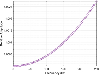
Figure 3. The difference between the mean pressure over hydrophone element and the calculated uniform pressure in the coupler.
Download figure:
Standard image High-resolution image2.2.2. Drive system.
While it would be more typical for a pistonphone to be driven by an electric motor or moving coil transducer, and for the pistonphone to be situated horizontally [14], the NPL pistonphone is driven by a piezoelectric stack and is oriented vertically. The piezoelectric actuator used to drive the piston is a 40 mm long stack of piezoelectric rings that, when driven with a constant sinusoidal voltage, cause the piston to move in and out of the sealed chamber. The total displacement of the piston varies depending on frequency, and in the operating frequency range of 0.5 Hz to 250 Hz the maximum displacement is a few micrometres, and typically is within 500 nm to 600 nm (there is approximately 4 Pa of sound pressure for 1 µm of piston displacement). The ceramic material used in the piezoelectric stack works best under compression to avoid potential fracture of the material and improve linearity. The stack is pre-stressed by the action of two pairs of back-to-back Belleville washers combined in series and compressed by a nut as per the manufacturer's recommendation.
Recalling that the piston displacement is measured at the base of this bolt, the spring washers and stiffness of the bolt itself serve to decouple the motion of the piston from the motion of the bolt. These components are securely assembled and are not altered during regular use. The small difference in displacement between the bolt and the piston face is due entirely to these stiffnesses and is assumed not to change, within the estimated uncertainty allowance, while the assembly remains intact. The difference must therefore be characterised and corrected for. A dual interferometer setup was implemented for this purpose with the first interferometer measuring the displacement at the base of the bolt, and the second simultaneously measuring the displacement on the piston face with the chamber opened. Since the difference is due to the mechanical setup of the piston and its drive system, this is assumed not to change once assembled, and the correction to the measured displacement need only be determined once per assembly (the assembly is not altered when opening the top lid or changing out the hydrophone). The ratio of piston displacement to the measured displacement was found to be 0.988.
2.2.3. The optical interferometer.
The primary route to traceability for length metrology is optical interferometry [28]. The NPL pistonphone uses a modified version of the NPL homodyne Michaelson optical interferometer [29] that is illuminated with a helium neon laser (Melles Griot Model:05-LHP-213). The optical components of the Michelson interferometer are two retroreflecting corner cubes and an NPL-produced phase quadrature beamsplitter. This beamsplitter is made from two right angle prisms one of which has had its hypotenuse face coated with successive thin layers of chrome, gold and chrome again prior to cementing the two prisms together [30]. The layers of thin metal films introduce a quadrature phase shift between incident laser light that is transmitted and reflected from the beamsplitter.
The transmitted component is incident on a fixed corner cube and retroreflected back to the beamsplitter, with the reflected component incident on a corner cube mounted on the bolt as described in the previous paragraph. As the bolt, and hence the corner cube, are displaced by the piezo electric actuator, the optical path length between the beam splitter and the moving corner cube changes. When both the fixed beam and the moving beam return to the beamsplitter they are displaced from the original beams and are recombined and interfere with each other. This recombined beam with an interference signal is then split by the beamsplitter into a reflected and a transmitted component, both of which have a component from the fixed and the moving beams that interfere with each other. The transmitted and reflected interfering beams have an approximate 90° phase difference between them. As the moving corner cube is displaced though a distance of half the wavelength of the light (316 nm), the intensity of the interfering beams varies sinusoidally producing optical fringes.
By counting the number of sinusoidal periods (fringes) traversed, each with a period of half the wavelength (316 nm), the displacement of the corner cube can be determined. However, owing to the phase quadrature coating, the reflected and transmitted beams with the recombined interfering signals beams correspond to approximately a sine and cosine signal. By calculating the four-quadrant inverse tangent of the sine signal divided by the cosine signal, it is possible to calculate the instantaneous phase of the interference signal. This enables interpolation of the optical fringes, such that the 316 nm fringe spacing may be subdivided allowing greater precision and the direction of motion may be determined. These beams are incident on two photodiodes that are connected to conditioning electronics in the controller unit which generate two signals such that the amplitude of the interference signal can vary between ±10 V as the moving corner cube travels through one optical fringe. The signals are collected using the Picoscope acquisition system and are post processed. As the signals are only approximately in phase quadrature, there will be a phase error term lending to non-linearity in the interferometer which may be corrected using a Heydeman correction [31, 32].
2.2.4. Measurement methodology.
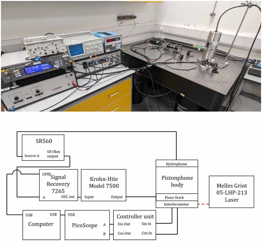
The experimental set up is shown in figure 4. The piezoelectric stack in the pistonphone body is driven by a sinusoidal signal generated at 0.5 V by a Signal Recovery 7265 lock-in amplifier and then amplified by 10x using a Krohn-Hite 7500 amplifier. The lock-in amplifier is also used to measure the output voltage from the hydrophone which is first pre-amplified using a Stanford Research SR560 preamplifier. The interferometer diode signals are put through the controller unit which are then measured by the picoscope measurement methodology. The picoscope & lock-in amplifier are connected to a computer via USB which uses code written in MATLAB to acquire and analyse the data.
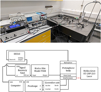
Figure 4. A photograph & block diagram of the laser pistonphone set up at NPL.
Download figure:
Standard image High-resolution imageBefore a calibration, the static pressure is measured when the chamber valve is open. It is then closed for the duration of the calibration, whereupon the static pressure within the pistonphone can be assumed constant, even if the external ambient pressure changes. The temperature and atmospheric pressure in the laboratory are recorded in the metadata for the measurement so that they can be used in the sensitivity calculation.
The measurement process from 0.5 Hz to 250 Hz in decidecade bands (one third octave bands, base 10) takes approximately 30 min, with the lowest frequency points taking the longest time to measure. The displacement is calculated from the interferometer diode signals as described in section 2.2.3 and the ratio applied to correct for the displacement location (at the bolt compared to the piston face). Using the displacement, the pressure in the cylindrical volume and then the sensitivity of the hydrophone is then calculated (following the method in section 1). Finally, three corrections are applied to the calculated hydrophone sensitivity.
2.2.5. Corrections to hydrophone sensitivity.
When deploying instrumentation in this low frequency range, the influence of AC-coupling can significantly alter the attempts to measure the signal. AC-coupling typically uses series capacitors to prevent DC signals from entering the measurement circuitry, but when a resistor is also present, the combination leads to a high-pass filter typically with a corner frequency of a few hertz—just the range where measurements are being attempted. Some instruments provide a DC-coupling option that avoids the problem, but care is needed to avoid DC signals. In other instruments the AC-coupling is inherent in the design, and needs to be characterised. This is the case with the lock-in amplifier model in use. Characterisation of the influence is a straight-forward matter of supplying the device with a constant level signal of variable frequency and measuring the indicated output. The correction applied to the hydrophone sensitivity is shown in figure 5 below.
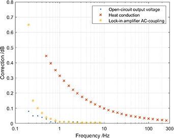
Figure 5. Measured corrections due to open-circuit output voltage, lock-in amplifier AC coupling, and heat conduction. The heat conduction correction has calculated using the model given in IEC 61 094–2 [26].
Download figure:
Standard image High-resolution imageThe electrical impedance of capacitive transducers such as hydrophones can become extremely high at low frequencies, with consequent risk of output signal attenuation due to electrical loading at the preamplifier input. When the calibration of the hydrophone refers to the open-circuit output voltage it is necessary to characterise the loading effect and correct for it. The substitution or insert-voltage method is a means of measuring the effective open-circuit output voltage from the hydrophone and can be implemented using the arrangement shown in figure 6.
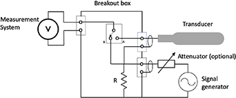
Figure 6. Arrangement for determining an open-circuit voltage correction.
Download figure:
Standard image High-resolution imageNote however that the procedure described is not necessary when the calibration refers to the output voltage of the complete system when any loading effects are an inherent part of the system's response.
The breakout box enables a low-value resistor R (conventionally 600 Ω is used) to be placed in series with the transducer. The input to the measurement system then cannot detect whether the applied voltage originates from the transducer or the low impedance source, but its input sees the same impedance load regardless of where the applied voltage is generated. With the switch in position A on the breakout box, the transducer is driven acoustically and the measurement system output is noted. Then, with the acoustic stimulus removed, the system is driven by the signal generator and the level adjusted until the measurement system reads as it did previously. Next, placing the switch in position B and leaving the signal generator unaltered, the voltage generated across the resistor can be measured. Since the resistor has a sufficiently low impedance, the measurement system is easily capable of measuring without losses, and the resulting voltage is equivalent to the open-circuit output voltage of the hydrophone.
In practice when seeking a correction for the effect, the first step in the process described above proves to be unnecessary. The open-circuit voltage correction is given by the ratio of the measurement system voltage when driven by the signal generator in switch position B, to that in switch position A. Note that while there is now no need to drive the hydrophone acoustically, the correction is best determined with the hydrophone mounted in the (inactive) pistonphone, as this provides the necessary acoustic isolation.
A correction must be determined for individual hydrophones. However, the correction is not expected to change for a given hydrophone and preamplifier combination, and this has been verified by periodic measurements spanning 6 months. The open-circuit output voltage correction for the hydrophone used in this study is shown in figure 5.
3. Results
A reference hydrophone was calibrated in the NPL pistonphone on several occasions over a period of 8 months, resulting in some 18 independent responses determined. A typical calibration included measurements in the frequency range 0.5 Hz to 500 Hz allow the high frequency limitations of the pistonphone to be evaluated. The measured sensitivity above 250 Hz deviated significantly from expectations and showed a significantly degraded level of repeatability, with the standard deviation of repeated measurements exceeding 1 dB. This is because sound pressure becomes increasingly non-uniform within the chamber at higher frequencies.
4. Measurement uncertainty
Factors affecting the determination of a hydrophone sensitivity using the pistonphone arise from electrical, mechanical, optical, acoustical and environmental considerations. The factors in each of these categories has been carefully examined, and the related uncertainty components identified and component values have been estimated. The most significant uncertainty components are summarised below, and the components and their relative contributions are given at selected frequencies in table 1, with the expanded (k = 2) combined uncertainty error bars shown in figure 7.
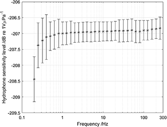
Figure 7. Average sensitivity of the 8104 reference hydrophone measured in the NPL pistonphone. Error bars represent the total expanded uncertainty (k = 2).
Download figure:
Standard image High-resolution imageTable 1. Uncertainty budget for hydrophone calibration by calculable pistonphone at NPL.
| Source of uncertainty | Frequencies of measurement (Hz) | |||||||||||||||||||||||||||||||
|---|---|---|---|---|---|---|---|---|---|---|---|---|---|---|---|---|---|---|---|---|---|---|---|---|---|---|---|---|---|---|---|---|
| 0.5 | 1.0 | 1.6 | 2.0 | 5.0 | 10.0 | 20.0 | 50.0 | 80.0 | 100.0 | 125.0 | 160.0 | 200.0 | 250.0 | |||||||||||||||||||
| Prob. Dist. | Divisor | ci | vi veff | value % | ui % | value % | ui % | value % | ui % | value % | ui % | value % | ui % | value % | ui % | value % | ui % | value % | ui % | value % | ui % | value % | ui % | value % | ui % | Value % | ui % | value % | ui % | value % | ui % | |
| Hydrophone preamplifier gain | Normal | 1.00 | 1.0 | infinity | 0.05 | 0.05 | 0.05 | 0.05 | 0.05 | 0.05 | 0.05 | 0.05 | 0.05 | 0.05 | 0.05 | 0.05 | 0.05 | 0.05 | 0.05 | 0.05 | 0.05 | 0.05 | 0.05 | 0.05 | 0.05 | 0.05 | 0.05 | 0.05 | 0.05 | 0.05 | 0.05 | 0.05 |
| Hydrophone loading (insert volt) | Normal | 1.00 | 1.0 | infinity | 0.20 | 0.20 | 0.06 | 0.06 | 0.06 | 0.06 | 0.06 | 0.06 | 0.03 | 0.03 | 0.00 | 0.00 | 0.00 | 0.00 | 0.00 | 0.00 | 0.00 | 0.00 | 0.00 | 0.00 | 0.00 | 0.00 | 0.00 | 0.00 | 0.00 | 0.00 | 0.00 | 0.00 |
| Lock-in amp ac coupled fr. resp. | Normal | 1.00 | 1.0 | infinity | 0.25 | 0.25 | 0.06 | 0.06 | 0.06 | 0.06 | 0.03 | 0.03 | 0.03 | 0.03 | 0.00 | 0.00 | 0.00 | 0.00 | 0.00 | 0.00 | 0.00 | 0.00 | 0.00 | 0.00 | 0.00 | 0.00 | 0.00 | 0.00 | 0.00 | 0.00 | 0.00 | 0.00 |
| Lock in amp calibration | Uniform | 1.73 | 1.0 | infinity | 0.05 | 0.03 | 0.05 | 0.03 | 0.05 | 0.03 | 0.05 | 0.03 | 0.05 | 0.03 | 0.05 | 0.03 | 0.05 | 0.03 | 0.05 | 0.03 | 0.05 | 0.03 | 0.05 | 0.03 | 0.05 | 0.03 | 0.05 | 0.03 | 0.05 | 0.05 | 0.05 | 0.03 |
| Electrical noise (pick up) | Uniform | 1.73 | 1.0 | infinity | 0.10 | 0.06 | 0.10 | 0.06 | 0.10 | 0.06 | 0.10 | 0.06 | 0.10 | 0.06 | 0.10 | 0.06 | 0.10 | 0.06 | 0.50 | 0.29 | 0.10 | 0.06 | 0.20 | 0.12 | 0.10 | 0.06 | 0.10 | 0.06 | 0.10 | 0.06 | 0.10 | 0.06 |
| Non-uniform pressure | Uniform | 1.73 | 1.0 | infinity | 0.00 | 0.00 | 0.00 | 0.00 | 0.00 | 0.00 | 0.00 | 0.00 | 0.00 | 0.00 | 0.00 | 0.00 | 0.01 | 0.01 | 0.02 | 0.01 | 0.03 | 0.01 | 0.04 | 0.02 | 0.07 | 0.04 | 0.12 | 0.07 | 0.18 | 0.10 | 0.30 | 0.17 |
| Optical interferometer | Normal | 1.00 | 1.0 | infinity | 2.00 | 2.00 | 1.60 | 1.60 | 1.60 | 1.60 | 1.20 | 1.20 | 1.20 | 1.20 | 1.20 | 1.20 | 1.20 | 1.20 | 1.20 | 1.20 | 1.20 | 1.20 | 1.20 | 1.20 | 1.20 | 1.20 | 1.20 | 1.20 | 1.20 | 1.20 | 1.20 | 1.20 |
| Correction washer-to-piston | Uniform | 1.73 | 1.0 | infinity | 2.00 | 1.15 | 2.00 | 1.15 | 2.00 | 1.15 | 2.00 | 1.15 | 2.00 | 1.15 | 2.00 | 1.15 | 2.00 | 1.15 | 2.00 | 1.15 | 2.00 | 1.15 | 2.00 | 1.15 | 2.00 | 1.15 | 2.00 | 1.15 | 2.00 | 1.15 | 2.00 | 1.15 |
| Vibration | Uniform | 1.73 | 1.0 | infinity | 0.50 | 0.29 | 0.50 | 0.29 | 0.50 | 0.29 | 0.50 | 0.29 | 0.50 | 0.29 | 0.50 | 0.29 | 0.50 | 0.29 | 0.50 | 0.29 | 0.50 | 0.29 | 0.50 | 0.29 | 0.50 | 0.29 | 0.50 | 0.29 | 0.50 | 0.29 | 0.50 | 0.29 |
| Chamber volume (V0) | Uniform | 1.73 | 1.0 | infinity | 0.50 | 0.29 | 0.50 | 0.29 | 0.50 | 0.29 | 0.50 | 0.29 | 0.50 | 0.29 | 0.25 | 0.14 | 0.50 | 0.29 | 0.50 | 0.29 | 0.50 | 0.29 | 0.50 | 0.29 | 0.50 | 0.29 | 0.50 | 0.29 | 0.50 | 0.29 | 0.50 | 0.29 |
| Static pressure (P0) | Uniform | 1.73 | 1.0 | infinity | 0.20 | 0.12 | 0.20 | 0.12 | 0.20 | 0.12 | 0.20 | 0.12 | 0.20 | 0.12 | 0.20 | 0.12 | 0.20 | 0.12 | 0.20 | 0.12 | 0.20 | 0.12 | 0.20 | 0.12 | 0.20 | 0.12 | 0.20 | 0.12 | 0.20 | 0.12 | 0.20 | 0.12 |
| Ratio specific heats | Uniform | 1.73 | 1.0 | infinity | 0.05 | 0.03 | 0.05 | 0.03 | 0.05 | 0.03 | 0.05 | 0.03 | 0.05 | 0.03 | 0.05 | 0.03 | 0.05 | 0.03 | 0.05 | 0.03 | 0.05 | 0.03 | 0.05 | 0.03 | 0.05 | 0.03 | 0.05 | 0.03 | 0.05 | 0.03 | 0.05 | 0.03 |
| Non-uniform piston motion | Uniform | 1.73 | 1.0 | infiinty | 0.50 | 0.29 | 0.50 | 0.29 | 0.50 | 0.29 | 0.50 | 0.29 | 0.50 | 0.29 | 0.50 | 0.29 | 0.50 | 0.29 | 0.50 | 0.29 | 0.50 | 0.29 | 0.50 | 0.29 | 0.50 | 0.29 | 0.50 | 0.29 | 0.50 | 0.29 | 0.50 | 0.29 |
| Heat conduction correction | Uniform | 1.73 | 1.0 | infinity | 1.00 | 0.58 | 0.50 | 0.29 | 0.50 | 0.29 | 0.50 | 0.29 | 0.50 | 0.29 | 0.50 | 0.29 | 0.50 | 0.29 | 0.50 | 0.29 | 0.50 | 0.29 | 0.50 | 0.29 | 0.50 | 0.29 | 0.50 | 0.29 | 0.50 | 0.29 | 0.50 | 0.29 |
| Type A repeatability | Normal | 1.00 | 1.0 | 17 | 1.00 | 1.00 | 0.50 | 0.50 | 0.30 | 0.30 | 0.25 | 0.25 | 0.25 | 0.25 | 0.25 | 0.25 | 0.25 | 0.25 | 1.00 | 1.00 | 0.25 | 0.25 | 0.25 | 0.25 | 0.50 | 0.50 | 0.50 | 0.50 | 0.50 | 0.50 | 1.00 | 1.00 |
| Combined uncertainty (%) | Normal | 2.67 | 2.12 | 2.09 | 1.79 | 1.79 | 1.77 | 1.79 | 2.05 | 1.79 | 1.79 | 1.84 | 1.84 | 1.84 | 2.04 | |||||||||||||||||
| Expanded uncertainty [k = 2] (%) | Normal | 5.33 | 4.25 | 4.17 | 3.58 | 3.57 | 3.54 | 3.57 | 4.10 | 3.57 | 3.58 | 3.68 | 3.68 | 3.68 | 4.08 | |||||||||||||||||
| Expanded uncertainty [k = 2] (dB) | Normal | 0.45 | 0.36 | 0.35 | 0.31 | 0.31 | 0.30 | 0.30 | 0.35 | 0.30 | 0.31 | 0.31 | 0.31 | 0.31 | 0.35 | |||||||||||||||||
The uncertainty components may be categorised by inspection of the experimental model shown equations (1)–(3) and may be considered to fall into two parts: (i) measurement of the response of the sensor being calibrated—essentially this involves electrical measurement of the hydrophone voltage (though in the case of the validation exercises, the sensor could be a microphone); (ii) the determination of the pressure inside the chamber to which the sensor is exposed—essentially this part is the realisation of the acoustic pascal within the chamber. This latter part may again be subdivided into the determination of the piston motion (using the optical interferometer) and the determination of the acoustic impedance of the chamber (which depends upon mechanical and environmental factors). These component values have been expressed as uniform distributions unless they are a result of independent measurements (where they will be expressed as a normal distribution). Finally, there is the repeatability of the calibration (the Type A uncertainty) expressed as a normal distribution and calculated from the standard deviation of the calibration results.
Considering the factors affecting the hydrophone, the output voltage of the hydrophone is used directly to determine the sensitivity. A calibrated lock-in amplifier is used to measure the hydrophone output voltage with the uncertainty on the calibration of 0.05% in the frequency range 0.5 Hz to 250 Hz. Since corrections for the frequency response of the lock-in amplifier input and the impedance loading influence of the hydrophone preamplifier are applied to the calculation of the hydrophone sensitivity, the uncertainties in the corrections are also considered. For the lock-in amplifier, the uncertainty ranges from 0.25% at 0.5 Hz to 0.03% at 50 Hz, and for the insert voltage correction for the preamplifier impedance loading, the uncertainty ranges from 0.20% at 0.5 Hz to 0.03% at 50 Hz, with both uncertainties being negligible at higher frequencies. In addition, there is the uncertainty to account for the non-uniform pressure across the element of the hydrophone (a spatial-averaging effect). No correction was applied for this small effect, but an uncertainty was estimated from the finite element modelling ranging from 0.02% at 50 Hz to 0.3% at 250 Hz. Electrical noise on the hydrophone signal was minimised by the use of the lock-in amplifier and signal averaging, and the residual is minimal except around the electrical supply frequency of 50 Hz.
The determination of the pressure in the chamber is dependent on the measurement of the displacement of the piston, which is turn depends upon several factors. The measurement uncertainty associated with the determination of displacement from the interferometer, including both the optical wavelength and the processing of the orthogonal optical signals, was estimated to be 24 nm [28–30]. The displacements generated for the measurements described here were limited to a maximum of a few micrometres, leading to uncertainties of 2% at 0.5 Hz and 1.2% above 5 Hz. The interferometer mirrors and lenses are susceptible to vibration leading to some residual spurious displacement components which have a greater effect at the lower frequencies. In addition, the displacement is measured for the corner cube positioned on the Belleville washer external to the piston. The lack of total rigidity between the two positions leads to a slight difference in displacement, which was tested using a bespoke set of optics to divide the optical beams and measure the displacement of the piston face and the washer simultaneously with the chamber end cap removed. The difference was found to be 1.25% which is applied as a displacement correction, with an conservative uncertainty value of 2% included to account for the potential for variation in the value across the frequency range and between checks of the correction performed using the interferometer. Finally, the motion of the piston face may not be uniform across its diameter. This was tested by scanning the face using a scanning vibrometer (Polytec PSV-400) during operation (again, with the end cap removed). The piston displacement was found to be uniform to within 1% across the diameter, leading to a negligible uncertainty contribution.
Calculation of the pressure to which the hydrophone is exposed requires the determination of the acoustic impedance, the uncertainty of which depends upon several factors. Environmental factors include ambient pressure and the ratio of specific heats for air, both of which enter the calculation of the pressure in the chamber directly. Temperature fluctuation can lead to sound pressure instabilities in the closed cavity, but these are reflected in the measurement repeatability. Ambient pressure is measured in the laboratory space and the static pressure in the pistonphone cavity is assumed to be equalised to the ambient pressure. A valve is opened to the atmosphere at the start of each measurement, and once closed the pressure is assumed to be stable for the duration of the test. A fixed value of 1.4 is used for the ratio of specific heats during calibrations but is in practice a function of the environmental conditions [33], and varies between 1.4000 to 1.4007 over the range of ambient conditions in the laboratory, leading to a negligible uncertainty contribution.
Mechanical factors include the cavity length and cavity diameter which are used to calculate the volume, on the basis that the cavity is a perfect cylinder. Therefore, the uncertainty in a diameter measurement, the roundness of the cross section and the longitudinal variation in diameter, and the uncertainty in the cavity length and parallelism of the end cap and piston, all contribute to the uncertainty in the derived volume. Additional volume elements from voids or intrusion into the cavity are also be taken into account. There is also uncertainty in estimating the amount of volume to be added or subtracted to account for the hydrophone volume which contributes to the uncertainty in the cavity volume. The piston diameter is also used to determine the excitation volume velocity, so uncertainty in the diameter measurement and roundness contribute to the overall uncertainty.
Acoustical factors include the assumption of adiabatic conditions during the process, which is valid at sufficiently high frequencies. However, the low operating frequencies of the pistonphone are within the adiabatic-to-isothermal transition region, and a heat conduction correction is required for the departure from adiabatic conditions. IEC 61 094–2 [26] specifies a model for the transition towards isothermal behaviour and this model is used to derive a correction to the calculated sound pressure. The uncertainty in the model calculations has been estimated in other studies and a similar value is used here [22, 24]. The formula also assumes that the cavity is a pure acoustic compliance and is therefore completely sealed. Any pressure leakage represents an acoustic resistance in parallel with the compliance, causing a roll-off in the generated sound pressure for the same volume velocity from the piston, as the frequency reduces. The amount of sound pressure reduction is determined by the product of the acoustic compliance and acoustic resistance, and therefore the leakage time constant. The leakage time constant (the time for the pressure to fall to 1/√2 or 71% of its initial value), has been tested by monitoring the decay in raised static pressure and estimated to be of the order of several hours, resulting in a negligible uncertainty component.
Finally, uncertainty due to experimental factors include the repeatability in both the piston displacement and the hydrophone output voltage measurements during a calibration. These have been assessed individually, but manifest as the experimental repeatability in successive sensitivity determinations (typically 4 or more) of the hydrophone under test under the same nominal conditions. A reference hydrophone has been calibrated repeatedly over a period of several months to derive a representative value for the experimental repeatability.
Table 1 shows the estimated values for the uncertainties at selected frequencies in the range from 0.5 Hz to 250 Hz. They are expressed as standard uncertainties in percent.
These uncertainty components are assumed to be uncorrelated, and have been combined according to established practices [34] to obtain the overall measurement uncertainty associated with the calibration. An expanded uncertainty has been calculated using a coverage factor of k = 2, corresponding to a confidence interval of approximately 95%. This expanded uncertainty ranges from 0.45 dB at 0.5 Hz to 0.35 dB at 250 Hz, with an optimal uncertainty of 0.30 dB in the mid-frequency range of 10 Hz to 100 Hz.
5. Validation and discussion
As a first step, confidence in the performance of the pistonphone is supported by the measured response of the hydrophone used in the development. The measured sensitivity as a function of frequency (the frequency response) meets expectations that the hydrophone has a nominally flat response over the operating frequency range of the pistonphone, specified by the manufacturer as ±1.5 dB from 0.1 Hz to 10 kHz (with the hydrophone exhibiting the nominal flat response at frequencies up to 10 kHz). The magnitude of the sensitivity has also been found to match the nominal value for higher frequencies. However, this in itself is not sufficient validation.
The calculable pistonphone provides a means of absolute calibration, and since there are currently no alternatives covering this frequency range, this is raised to a primary calibration method. Ideally then, the validation process requires comparisons to be carried out with other realisations of primary calibration methods. However, to the knowledge of the authors, there are no equivalent calibration capabilities for hydrophones available globally, that are in a suitably developed state for such a comparison.
Pre-empting this gap in technical capability, the pistonphone was designed to also calibrate measurement microphones, thereby opening the possibility to validate its performance via existing microphone calibration capabilities.
Prior to the development of the pistonphone, hydrophones have been calibrated at NPL by comparison with a measurement microphone using a different calibration facility. Traceability for hydrophone calibration was therefore to a reference microphone calibrated at the Danish National Metrology Institute (DFM). This microphone calibration covered the frequency range from 2 Hz to 20 kHz, and therefore overlaps with part of the operating frequency range of the pistonphone, providing the opportunity for a comparison with DFM.
The reference microphone is a Brüel and Kjær type 4134 fitted with a UA0825 adapter ring (see figure 8), which converts the microphone into the laboratory standard configuration suitable for reciprocity calibration [26] implemented at DFM.

Figure 8. The Brüel and Kjær type 4134 microphone with its regular protection grid (left), and UA0825 adapter (right) for converting to laboratory standard configuration. The microphone pressure-equalisation vent outlet is visible just above the thread.
Download figure:
Standard image High-resolution imageFigure 9 shows the sensitivity of the microphone determined with the NPL pistonphone and by reciprocity calibration at DFM. The difference in the results and the associated measurement uncertainty is plotted in figure 11. The measurement uncertainty for the NPL measurements is similar to that for a hydrophone calibration (see Table uncertainty), and for the DFM measurements is typically 0.13 dB at 2 Hz decreasing to 0.03 dB above 125 Hz.

Figure 9. Results of comparison of microphone calibration at NPL and DFM.
Download figure:
Standard image High-resolution imageSince this was an opportunistic comparison, there is a 20 month time span between the calibrations, during which the microphone was used for other purposes, which might explain the approximately constant difference of 0.04 dB to 0.06 dB above 30 Hz. Nevertheless, this level of equivalence is within the combined measurement uncertainty of 0.3 dB of the two calibrations. Below 30 Hz, the NPL results are seen to roll off, and the difference exceeds the combined measurement uncertainty below 3 Hz.
The frequency response of a measurement microphone in the frequency region below approximately 30 Hz, is strongly influenced by the mechanism used to equalise static pressure within the microphone, to that in the external environment. When the microphone measures low-frequency sound pressure in a closed cavity such as presented by the pistonphone, the effective sensitivity depends critically on whether or not the pressure-equalisation vent is exposed to the sound pressure.
For the calibration at DFM, the normal protection grid is replaced with a UA0825 adapter, designed to seal to the outer rim of the microphone diaphragm. Such an adapter usually facilitates pressure calibration where the stimulus is confined only to the diaphragm of the microphone, as in coupler reciprocity calibration for example. During reciprocity calibration, the face of the adapter ring mates with the calibration coupler to ensure that the sound pressure does not reach the pressure-equalisation vent.
However, in the NPL pistonphone it is unlikely that the face of the UA0825 adapter is completely sealed to the pistonphone cavity, and sound pressure inevitably reaches the body of the microphone, including the pressure-equalisation vent. This difference between the two calibrations is likely to account for the deviations observed in the results.
While the comparison with DFM was opportunistic, a second comparison with the Laboratoire National de Métrologie et d'Essais (LNE) was arranged specifically for the validation of the NPL pistonphone. LNE have developed their own pistonphone for microphone calibration [24].
A microphone system comprising a Brüel and Kjær type 4134 microphone, a GRAS type 26AK preamplifier and Vinculum type E711 microphone power supply, was sent to LNE for calibration as a system in the LNE pistonphone. In this case the microphone was fitted with its regular protection grid (see figure 8), so that under normal circumstances, and crucially in both calibration devices, the pressure-equalisation vent is exposed to the sound pressure.
LNE calibrated the microphone in the frequency range from 0.1 Hz to 20 Hz. Consequently, the usual measurement frequency range of the NPL pistonphone was extended to 0.2 Hz, to gain as much knowledge from the comparison as possible.
The measurement uncertainty of the LNE results is 0.1 dB at 0.2 Hz, decreasing to 0.04 dB at 4 Hz and above.
Figure 10 shows that the sensitivity of this reference microphone system rolls off strongly as the frequency decreases due to the pressure-equalisation vent exposure to the sound pressure. As before, the difference in the results and the associated measurement uncertainty is plotted in figure 11. The strong roll-off in the response might suggest that the degrading signal-to-noise ratio could be the cause of the observed differences. Note however, that the signal levels here are still higher than experienced in a hydrophone (see figure 7).
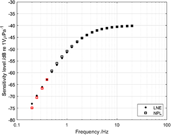
Figure 10. Results of comparison of microphone calibration at NPL and LNE. Results below 0.5 Hz are outside of the targeted operating range of the NPL pistonphone and therefore indicated in red.
Download figure:
Standard image High-resolution image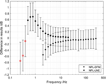
Figure 11. Differences from the microphone calibration comparisons between NPL and DFM, and NPL and LNE. Results below 0.5 Hz are outside of the targeted operating range of the NPL pistonphone so are shown in red.
Download figure:
Standard image High-resolution image
Again, there is good equivalence at frequencies above 4 Hz. However, the onset of an unknown influence begins at 4 Hz and increases to almost 0.7 dB at 0.8 Hz. Such behaviour is not evident in the frequency response of the NPL reference hydrophone (see figure 7), or in the results of the comparison with DFM. The performance of the LNE pistonphone is likewise validated by comparison with other calibration methods both at LNE and at other National Measurement Institutes. Since there is other evidence ruling out the performance of the calibration devices themselves, the observed differences are likely due to subtle changes in the microphone system exchanged between LNE and NPL; the change perhaps arising from transportation, as the trend has been persistent in all measurements since the reference microphone system returned from calibration at LNE. Additional measurements are necessary to investigate these findings further.
In summary then, the strongest evidence validating the performance of the pistonphone from 0.5 Hz to 4 Hz is that measurements on the NPL reference hydrophone produce the expected flat (within ±0.1 dB) frequency response. Validation is further supported by the results of the microphone calibration comparisons with DFM and LNE, where the results compare well when not influenced by artifacts produced by the microphone itself (above 3 Hz for DFM and 1.6 Hz for LNE). Additional measurements are required to achieve complete validation below 1.6 Hz.
6. Conclusion
This paper presents a new design and comprehensive uncertainty analysis for establishing primary standards for hydrophone calibration at low frequencies from 0.5 Hz to 250 Hz, with expanded uncertainties ranging from 0.45 dB at 0.5 Hz to 0.30 dB at 20 Hz, and to 0.35 dB at 250 Hz (expressed for a coverage factor of k = 2). The design is based on a pistonphone where sound pressure is generated in a cavity with a fixed air volume by the motion of a piston, creating a well-defined volume velocity. The generated sound pressure is calculated from the acoustic impedance of the cavity and a measurement of the volume velocity, the latter being determined from the piston displacement which is measured using optical interferometry.
The approach to performance validation was to assess equivalence with independent validated methods. In fact, two methods were considered, both used to calibrate microphones (the chosen transfer standard device for the comparison). These alternative methods were the coupler reciprocity method at frequencies 2 Hz to 250 Hz, and another independent implementation of the calculable pistonphone method at another institute in the range 0.2 Hz to 20 Hz. The equivalences were demonstrated for modulus of sensitivity in the frequency range from 0.5 Hz to 250 Hz, with differences increasing for frequencies below 1 Hz with some as yet unexplained trends. These could be due to venting in the NPL calibration for the microphone used in the case of the comparison with DFM, and changes in the response of the microphone used to compare with LNE.
The pistonphone provides a capability to establish traceability to primary realisation of the pascal for sound pressure in underwater acoustics, this being the first validated example of a primary method based on such a calculable pistonphone design. The lack of validation of standards for low frequencies in underwater acoustics has been recognised by the consultative committee for acoustics ultrasound and vibration in its recent strategy [35]. Such primary methods will underpin future low frequency key comparisons organised under the auspices of the international committee of weights and measures (CIPM), and the validated measurement capabilities declared by metrology institutes within the BIPM Key Comparison Database [36] a crucial part of the infrastructure of the mutual recognition arrangement [37]. In the future, it is anticipated the system described in this paper can be extended to incorporate phase calibration.
Standards may now be disseminated by calibration of a wide variety of hydrophones using a comparison method in an enclosed coupler, with traceability provided for a range of low frequency applications. However, one limitation of the method described here is the inability to provide a realisation of the acoustic pascal over the range of environmental conditions that exist in the ocean, important for some deep water applications. For this, a method is needed that can simulate the depth (applied hydrostatic pressure) and temperature that pertains to deep ocean applications. One possible method to at least partly address this need is coupler reciprocity in a sealed fluid-filled chamber, which although challenging, is under development at several institutes [16].
Acknowledgments
Part of this work has received funding within the project 19ENV03 Infra-AUV from the EMPIR program co-financed by the participating states and from the European Union's Horizon 2020 research and innovation program.