

Abstract
Synchronization has received a lot of attention from the scientific community for systems evolving on static networks or higher-order structures, such as hypergraphs and simplicial complexes. In many relevant real-world applications, the latter are not static but do evolve in time, in this work we thus discuss the impact of the time-varying nature of higher-order structures in the emergence of global synchronization. To achieve this goal, we extend the master stability formalism to account, in a general way, for the additional contributions arising from the time evolution of the higher-order structure supporting the dynamical systems. The theory is successfully challenged against two illustrative examples, the Stuart–Landau nonlinear oscillator and the Lorenz chaotic oscillator.
Export citation and abstract BibTeX RIS

Original content from this work may be used under the terms of the Creative Commons Attribution 4.0 license. Any further distribution of this work must maintain attribution to the author(s) and the title of the work, journal citation and DOI.
1. Introduction
In the realm of complex systems, synchronization refers to the intriguing ability of coupled nonlinear oscillators to self-organize and exhibit a collective unison behavior without the need for a central controller [1, 2]. This phenomenon, observed in a wide range of human-made and natural systems [3], continues to inspire scientists seeking to unravel its underlying mechanisms.
To study synchronization, network science has proved to be a powerful and effective framework. Here, the interconnected nonlinear oscillators are represented as nodes, while their interactions are depicted as links [4]. However, the classical static network representation has its limitation in modeling many empirical systems, such as social networks [5], brain networks [6, 7], where the connections among individual basic units are adaptable enough to be considered to evolve through time. Therefore, the framework of networks has been generalized as to include time-varying networks [8, 9], whose connections vary with time. Scholars have thus studied synchronization on time-varying networks [10–12] and generalizations such as multilayer networks [13].
Another intrinsic limitation of networks is due to their capability to only model pairwise interactions. To go beyond this issue, scholars have brought to the fore the relevance of higher-order structures, which surpass the traditional network setting that models the interactions between individual basic units only through pairwise links [14–18]. By considering the simultaneous interactions of many agents, higher-order structures, namely hypergraphs [19] and simplicial complexes [20], offer a more comprehensive understanding of complex systems. These higher-order structures have been proven to produce novel features in various dynamical processes, including consensus [21, 22], random walks [23, 24], pattern formation [14, 25, 26], synchronization [14, 27–32], social contagion and epidemics [33, 34]. Nevertheless, the suggested framework is not sufficiently general to describe systems with many-body interactions that vary with time. As an example, group interactions in social systems have time-varying nature as the interactions among teammates are not always active but rather change throughout time [35]. Some early works have begun to investigate the time-varying aspect of many-body interactions in various dynamical processes. For instance, time-varying group interactions have been demonstrated to influence the convergence period of consensus dynamics [22] and to predict the onset of endemic state in epidemic spreading [34].
The present work is motivated by these recent research directions, and it aims to take one step further by considering the impact of time-varying higher-order structures in the synchronization of nonlinear oscillators. In this context, a preliminary effort has been reported in [36], where authors have investigated synchronization in time-varying simplicial complexes but limited to the fast switching case [37, 38] among distinct static simplicial configurations; namely the time scale of the simplicial evolution is exceedingly fast compared to that of the underlying dynamical system. In contrast, in the present work, we allow the higher-order structures to evolve in time without any constraint, thus removing any limitations on the imposed time evolution of the higher-order structure. We present the results in the framework of hypergraphs, but they hold true also for simplicial complexes, whenever we do not impose any assumption of regularity of the topology for the hypergraph, as we will show in the following.
Under such broad assumptions, we develop a theory to determine the conditions ensuring the stability of a globally synchronized state that generalizes the master stability function (MSF) [39] along two directions: we allow for higher-order structures and we let them to evolve in time. The generalized framework hereby presented, assumes that the coupling functions cancel out when the dynamics of individual oscillators are identical; let us observe that this is a necessary condition that must be met for the coupled system to have a global synchronous solution, namely to ensure the existence of a synchronous manifold, and it has been largely used in the literature across various domains. Let us recall that the general strategy to prove the existence of global synchronization relies on the study of the linear (non-autonomous) system obtained by linearizing the dynamics close to the homogeneous reference solution. Such system has (generally) a very large dimension and thus to simplify its analysis one can recur to the MSF by projecting on the eigenbasis of a suitable operator, often the Laplace matrix responsible for the diffusive-like coupling. In the case of time-varying higher-order structures, the eigenvectors also depend on time and thus they contribute to an 'extra term' to the MSF [12]. Anticipating on the following, we will show that the latter contribution can substantially modify the system behavior and neglecting it would determine wrong conclusions about synchronization. We present our results by using coupled Stuart–Landau (SL) oscillators and the paradigmatic Lorenz system; in a first phase we used a small toy time-varying hypergraph to allow us to emphasize the novelty of the proposed method without adding unnecessary complications, then we employed generic time-varying higher-order structures made of 100 and 200 nodes. The presented results support the claim that temporality in group interactions can induce synchronization earlier as compared to the static group interactions. Furthermore, our results also reveal that the combined effect of adequate temporality and strong enough group interactions can induce desynchronization in time-varying higher-order structures.
2. The model
Let us consider a m-dimensional dynamical system,  , whose time evolution is described by the following ordinary differential equation

where  denotes the system state vector and
  some smooth nonlinear function. Let us assume moreover that system (1) exhibits an oscillatory behavior, being the latter periodic or irregular; we are thus considering the framework of generic nonlinear oscillators. Assume to have n identical copies of system (1) coupled by a symmetric higher-order structure; namely, we allow the nonlinear oscillators to interact in couples, as well as in triplets, quadruplets, and so on, up to interactions among D + 1 units. We can thus describe the time evolution of the state vector of the ith unit by

where for  ,
,  denotes the coupling strength,
  the nonlinear coupling function and
  the tensor encoding which units are interacting together. More precisely
  if the units
  do interact at time t, observe indeed that such tensor depends on time, namely the intensity of the coupling as well which units are coupled, do change in time. Finally, we assume the time-varying interaction to be symmetric, namely if
  , then
  for any permutation π of the indexes
  . Let us emphasize that we consider the number of nodes to be fixed, only the interactions change in time; one could relax this assumption by considering to have a sufficiently large reservoir of nodes, from which the core of the system can recruit new nodes or deposit unused nodes.
Let us fix a periodic reference solution,  , of system (1). We are interested in determining the conditions under which the orbit
  is a solution of the coupled system (2), and moreover it is stable, namely any orbit whose initial conditions are sufficiently close to the reference solution will converge to the latter and thus the n units globally synchronize, i.e. they behave at unison. A necessary condition is that the coupling functions vanish once evaluated on such orbit, i.e.
  , for
, for  . This assumption is known in the literature as non-invasive condition.
For the sake of pedagogy, we will hereby consider a particular case of non-invasive couplings and we will refer the interested reader to appendix  to be diffusive-like, namely for each d there exists a function
  such that

In this way we can straightforwardly ensure that the coupling term in equation (3) vanishes once evaluated on the orbit  , allowing thus to conclude that the latter is also a solution of the coupled system. Stated differently there exists a synchronous manifold defined by
  .
.
To study the stability of the reference solution, let us now perturb the synchronous solution  with a spatially heterogeneous term, meaning that
  we define
  . Substituting the latter into equation (2) and expanding up to first order, we obtain

where

being  the generalized multi-indexes Kronecker-δ, and the (time-varying) d-degree of node i is given by

which represents the number of hyperedges of order d incident to node i at time t. Observe that if  is weighted, then
  counts both the number and the weight, it is thus the generalization of the strength of a node. Let us now define

namely the number of hyperedges of order d containing both nodes i and j at time t. Again, once  is weighted, then
  generalizes the link strength. Let us observe that because of the invariance of
  under index permutation, we can conclude that
  . Finally, we define the generalized time-varying higher-order Laplacian matrix for the interaction of order d as

Observe that such a matrix is symmetric because of the assumption on the tensors  . Let us also notice the difference in sign with respect to other notations sometimes used in the literature.
We can then rewrite equation (4) as follows
where we used the fact the  is independent from the indexes being the latter placeholders to identify the variable with respect to which the derivative has to be done. Finally, by defining

we can rewrite equation (8) in compact form

This is a non-autonomous linear differential equation allowing to determine the stability of the perturbation  , for instance, by computing the largest Lyapunov exponent. To make some analytical progress in the study of equation (9), we will consider in the following two main directions. First case, the functions
  satisfy the condition of natural coupling (see section 2.1), second case the higher-order structures exhibit regular topologies (see section 2.2). The aim of each assumption is to disentangle the dependence of the nonlinear coupling functions from the higher-order Laplace matrices and thus achieve a better understanding of the problem under study.
2.1. Natural coupling
Let us assume the functions  to satisfy the condition of natural coupling, namely

that implies  and it allows to eventually rewrite equation (9) as follows

where

Let us observe that the matrix  is a Laplace matrix; it is non-positive definite (as each one of the
  matrices does for any
  and any t > 0, and
  ), it admits
  as eigenvalue associated to the eigenvector
  because each
  does the same and it is symmetric, being
  also symmetric for all
  . So there exists an orthonormal time-varying eigenbasis,
  ,
,  , for
, for  with associated eigenvalues
  for
for  . The goal is to use those eigenvectors to project (11) and thus to obtain the MSF; however, as we observed in the introduction, because the eigenvectors vary in time we have to take into account their time dependence. To achieve this goal we thus define [12] the n × n time dependent matrix
  that quantifies the projections of the time derivatives of the eigenvectors onto the independent eigendirections, namely

By recalling the orthonormality condition

we can straightforwardly conclude that c is a real skew-symmetric matrix with a null first row and first column, i.e.  and
and  .
.
Based on the above reasoning and to make one step further, we consider equation (11), and we project it onto the eigendirections, namely we introduce  and recalling the definition of c we obtain

Let us observe that the latter formula and the following analysis differ from the one presented in [40] where the perturbation is assumed to align onto a single mode, a hypothesis that ultimately translates in the stationary of the Laplace eigenvectors that is  . The same assumption is also at the root of the results presented in [41]; indeed, commuting time-varying networks implies to deal with a constant eigenbasis. In conclusion, equation (14) returns the more general description for the projection of the linearized dynamics on a generic time-varying Laplace eigenbasis, and thus allowing us to draw general conclusions without unnecessary simplifying assumptions. Let us observe that we did not introduce any assumption of the time-varying hypergraph and in particular we did not impose that nodes belonging to a k-hyperedge necessarily belong also to all k'-hyperedges,
  contained in the former, as it should be for a simplicial complex. Namely the previous analysis applies to both hypergraphs and simplicial complexes. Stated differently the adjacency tensors
  , with
  are independent each other, condition that will be no longer true in the case of regular topologies as we will show in the next section.
2.2. Regular topologies
An alternative approach to study equation (9) is to assume regular topologies [25], namely hypergraphs such that  , for
, for  , with α1 = 1 and
  . The latter have been introduced in [25] to propose simple structures allowing for the emergence of Turing patterns; observe that tetrahedra or icosahedra are examples of regular topologies once we assume unweighted, i.e. binary, and static adjacency tensors, the same holds true for the triangular lattice with periodic boundary conditions, i.e. a two-torus paved with triangles. Let us also emphasize that such topologies should not be confused with the concept of regular network or regular hypergraph, where, i.e. all nodes have the same degree. In the case of higher-order structures, the adjective regular refers to the fact that higher-order Laplace matrices differ only by a multiplicative factor and thus they are simultaneously diagonalizable.
By the very first property of regular topologies, equation (9) can be rewritten as

where

that results in a sort of weighted nonlinear coupling term. We can now make use of the existence of a time-varying orthonormal basis of  , namely
  ,
,  , associated to eigenvalues
  ,
,  and
and  , to project
  onto the n eigendirections,
  . Because the latter vary in time we have again an extra term in the MSF and we thus need to define a second n × n time dependent matrix
  given by

that it is again real, skew-symmetric, with a null first row and first column, i.e.  and
and  , because of the orthonormality condition of eigenvectors. By projecting equation (15) onto
  , we get

Let us conclude by observing that the latter equation has the same structure of (14). Those equations determine the generalization of the MSF to the case of time-varying higher-order structures. The time variation signature of the topology is captured by the matrices  or
or  and the eigenvectors
  or
or  , while the dynamics (resp. the coupling) in the Jacobian Jf
(resp.
, while the dynamics (resp. the coupling) in the Jacobian Jf
(resp.  or
or  ).
).
It is important to notice that as the eigenvalues  ,
,  and the skew-symmetric matrices
  have null first row and column, in analogy with the MSF approaches carried over static networks [39] and higher-order structures [42], hence also in the case of time-varying higher-order structures, we can decouple the MSF into two components. One component describes the movement along the synchronous manifold, while the other component represents the evolution of different modes that are transverse to the synchronous manifold. The MSF ultimately relies on the computation of the maximum Lyapunov exponent (MLE) associated with the transverse modes and measures the exponential growth rate of a tiny perturbation in the transverse subspace. For the synchronous orbit to be stable, the MLE associated to all transverse modes must be negative. Moreover, the MSF approaches applied to static networks and higher-order structures can be simplified by examining the evolution of the perturbation along each independent eigendirection associated with distinct eigenvalues of the Laplacian matrix. Let us observe that this is not possible in the present because the matrices
  and
and  mix the different modes and introduce a complex interdependence among them, making it challenging to disentangle their individual contributions. For this reason, one has to address numerically the problem [12].
To demonstrate the above introduced theory and emphasize the outcomes arising from the modified MSF (14) and (18), we will present two key examples in the following sections. Indeed, we will utilize the SL limit cycle oscillator and the chaotic Lorenz system as prototype dynamical systems anchored to each individual node. To simplify the calculations, we assume that the hypergraph consists of only four nodes, five links and two three-hyperedges, i.e. triangles, whose weights change in time (see appendix  , with
  , namely
  . The latter ultimately implies dealing with a simplicial complex because of the presence of all k'-order connections,
  , among nodes once they belong to a given k-hypergraph.
3. Synchronization of SL oscillators coupled via time-varying higher-order networks
The aim of this section is to present an application of the theory above introduced. We decided to use the SL model as a prototype example because it provides the normal form for a generic system close to a supercritical Hopf-bifurcation and for this reason it has been largely used in the literature to study synchronization.
An SL oscillator can be described by a complex amplitude w that evolves in time according to  , where
  and
and  are complex model parameters. The system admits a limit cycle solution
  , where the frequency of the oscillation is given
  ; moreover the limit cycle is stable provided
  and
and  , conditions that we hereby assume.
To proceed in the analysis, we couple together n identical SL oscillators, each one described by a complex amplitude wj
, with  , anchored to the nodes of a time-varying hypergraph as prescribed in the previous section, namely

For the sake of simplicity, we restrict our analysis to pairwise and three-body interactions, namely D = 2 in equation (19). We hereby present and discuss the SL synchronization under the diffusive-like coupling hypothesis and by using two different assumptions: regular topology and natural coupling. The case of non-invasive coupling will be presented in appendix A.1.
3.1. Diffusive-like and regular topology
Let us thus assume the existence of two functions  and
and  such that
  and
and  do satisfy the diffusive-like assumption, namely

For the sake of definitiveness, let us fix

let us observe that the latter functions do not satisfy the condition for natural coupling, indeed  .
.
Let us assume to deal with regular topology, namely  . Hence following equation (16) we can define
  . Let us perturb the limit cycle solution
  by defining
  , where ρj
and θj
are real and small functions for all j. A straightforward computation allows to write the time evolution of ρj
and θj
once we restrict ourselves to consider only linear terms
, where ρj
and θj
are real and small functions for all j. A straightforward computation allows to write the time evolution of ρj
and θj
once we restrict ourselves to consider only linear terms

where  is the frequency of the reference limit cycle solution.
By exploiting the eigenvectors  and eigenvalues
  of
of  to project the perturbation ρj
and θj
we obtain:
to project the perturbation ρj
and θj
we obtain:

where the matrix b has been defined in equation (17),  is the sough projection and similarly for θβ
.
is the sough projection and similarly for θβ
.
As already mentioned, for the sake of definiteness and to focus on the impact of the time-varying topology, we hereby consider a simple higher-order network structure composed of n = 4 nodes, five links and two triangles with one link shared between both triangles. The number of nodes is thus fixed in time whereas the weight of the links and of the triangular face evolve in time. More precisely we consider the weights of the triangular faces to be given by  and
and  , where f(t) and g(t) are generic positive smooth functions and
  denotes any permutation of the indexes ijk. Whereas, the weights of the links, namely the pairwise adjacency matrix, are assumed to be given by

This provides us a regular hypergraph satisfying the relation  with
with  (see appendix
  corresponding to the zero eigenvalue. Consequently using the relation (17), we can obtain the skew symmetric projection matrix b such that all the entries of b are zero except
  (we refer the interested reader to appendix
To realize how time-varying regular structure affects the global synchronization phenomenon, we fix, without loss of generality, the functions determining the evolution of edges and triangular faces such that ![$f(t) = 1+[\sin(\Omega t)]^2$](https://content.cld.iop.org/journals/2632-072X/5/1/015020/revision3/jpcomplexad3262ieqn118.gif) and
and ![$g(t) = 1+[\cos(\Omega t)]^2$](https://content.cld.iop.org/journals/2632-072X/5/1/015020/revision3/jpcomplexad3262ieqn119.gif) . With this consideration, the case
. With this consideration, the case  corresponds to the static higher-order network structure and
  signifies the time-varying case. Figure B2 and the accompanying supplementary movie show the time evolution of the hypergraph structures for
  .
.
Under all these assumptions, equation (22) determines a time periodic linear system whose stability can be determined by using Floquet theory. In order to illustrate our results, we let  and
and  to freely vary in the range
 ![$[-1.5,1.5]$](https://content.cld.iop.org/journals/2632-072X/5/1/015020/revision3/jpcomplexad3262ieqn125.gif) and
and ![$[-2.5,2.5]$](https://content.cld.iop.org/journals/2632-072X/5/1/015020/revision3/jpcomplexad3262ieqn126.gif) , while keeping fixed to generic values the remaining parameters, and we compute the Floquet eigenvalue with the largest real part, corresponding thus to the MLE of equation (22), as a function of
, while keeping fixed to generic values the remaining parameters, and we compute the Floquet eigenvalue with the largest real part, corresponding thus to the MLE of equation (22), as a function of  and
and  . The corresponding results are shown in figure 1 for
  (panel (a)) and
  (panel (b)). By a direct inspection, one can clearly conclude that the parameters region associated with a negative MLE (black region), i.e. to the stability of the SL limit cycle and thus to global synchronization, is larger for
  than for
  in the regime of relatively smaller triadic coupling strength, i.e.
  small enough. However, for larger values of the latter, islands of positive MLE (yellow region) emerge for
  , i.e. for the time-varying higher-order structure.

Figure 1. Synchronization on time-varying regular higher-order network of coupled SL oscillators. We report the MLE as a function of  and
and  for two different values of Ω,
  (panel (a)) and
  (panel (b)), by using a color code, we determine the region of stability (black) and the region of instability (yellow). The remaining parameters have been fixed at the values
  ,
,  ,
,  ,
,  ,
,  .
.
Download figure:
Standard image High-resolution imageTo study the combined effect of both coupling strengths q1 and q2, we set  and
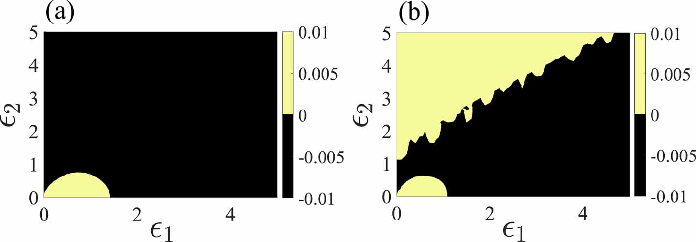
and  , and we compute the MLE as a function of ε1 and ε2, having fixed without loss of generality
  and
and  . The corresponding results are presented in figure 2 for static (
 , panel (a)) and time-varying (
 , panel (b)) higher-order structure. We can again conclude that the region of parameters corresponding to global synchronization (black region) is larger in the case of time-varying hypergraph than in the static case when the strength of triadic interactions is small enough. Conversely, when the strength of triadic interactions increases, the region of parameters supporting global synchronization contracts in the time-varying hypergraph case as opposed to the static counterpart.

Figure 2. Synchronization on time-varying regular higher-order network of coupled SL oscillators. The MLE is reported as a function of ε1 and ε2 for two different values of Ω,  (panel (a)) and
  (panel (b)). The color code represents the values of the MLE, negative values (black) while positive values (yellow). The remaining parameters have been fixed at the values
  ,
,  ,
,  ,
,  ,
,  .
.
Download figure:
Standard image High-resolution imageOur last analysis concerns the relation between the frequency Ω and the size of the coupling parameters ε1, ε2, still assuming  and
and  , on the onset of synchronization. In figure 3 we report the MLE in the plane
  for a fixed value of ε2 (panel (a)), and in the plane
  for a fixed value of ε1 (panel (b)). Let us observe that the synchronization can be easily achieved the smaller the value εj
,
for a fixed value of ε1 (panel (b)). Let us observe that the synchronization can be easily achieved the smaller the value εj
,  , for which the MLE is negative, having fixed Ω. Let us thus define
  , for fixed ε2, and similarly
  . The results of figure 3 clearly show that
  and
and  and thus support our claim that time-varying structures allow to achieve synchronization easier. However, for larger values of Ω, one can observe that the global synchronization is forbidden when the strength of three-body coupling ε2 is relatively larger (see figure 3(b)). Thus figure 3 illustrates that achieving synchronization is more attainable when the higher-order couplings are not overly intense. However, a noteworthy observation emerges: the interplay between a suitable level of higher-order coupling and temporality has the potential to induce desynchronization in higher-order structures.

Figure 3. Synchronization domains. We show the MLE in the plane  (panel (a)) for
  and in the plane
  (panel (b)) for
  . We can observe that in both panels, the critical value of coupling strengths
  to achieve synchronization is smaller for
  than for
  . The remaining parameters are kept fixed at the values
  ,
,  ,
,  ,
,  ,
,  .
.
Download figure:
Standard image High-resolution imageTo complement our analysis, we performed numerical simulations of the SL defined on the simple four nodes time-varying hypergraph. We selected  and the remaining parameters values as in figure 2, we can thus conclude that for the chosen parameters, the MSF is positive if
  and negative if
  , hence the SL should globally synchronize on the time-varying hypergraph while it would not achieve this state in the static case. Results of figure 4 confirm these conclusions; indeed, we can observe that (real part of) the complex variable is in phase for all i in the case
  (figure 4(b)), while this is not clearly the case for
  (figure 4(a)).

Figure 4. Time series of the signal  for a suitable choice of coupling parameters
  and
and  . In (a), we set
  while
while  in panel (b). The other parameters values are the same as in figure 2, i.e.
  ,
,  ,
,  ,
,  ,
,  .
.
Download figure:
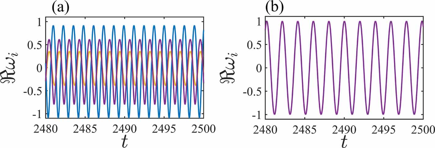
Standard image High-resolution imageFurthermore, to support the analytical insights suggesting that large values of Ω and ε2 lead to desynchronization in the time-varying higher-order structure, we conducted numerical simulations of the SL model defined on the same four-node time-varying hypergraph. Specifically, we set  while keeping the other parameter values as those used in figure 2. From the latter figure one can conclude that the MSF is negative if
  and positive if
  , hence the global synchronization is forbidden in the time-varying scenario. The findings presented in figure 5 validate this conclusion. Specifically, in the scenario where
  (figure 5(a)), the time series exhibit a synchronized state, as evidenced by the in-phase behavior of the real part of the complex variable across all nodes (i). On the contrary, this synchronized state is not observed in the case of
  (figure 5(b)), underscoring the influence of larger values of Ω and ε2 in inducing desynchronization within the system.

Figure 5. Time series of the signal  for a suitable choice of coupling parameters
  and
and  . In (a), we set
  while
while  in panel (b). The other parameters values are the same as in figure 2, i.e.
  ,
,  ,
,  ,
,  ,
,  .
.
Download figure:
Standard image High-resolution imageThe results obtained so far rely on the use of a small time-varying hypergraph composed by four nodes, we claim however that their validity goes beyond this simple framework. To support this statement, we studied generic random large hypergraphs obtained by using a slightly different approach than the presented above. Indeed, we assume the Laplace eigenvalues to be constant and the time-derivative of the associated eigenvectors projected on the eigenbasis to return a constant matrix b. Namely we generated 100 random skew-symmetric matrices b (with zeros in their first row and column), we assigned random sets of eigenvalues  and we numerically solve equation (22) to compute the MSF for the corresponding structures. Then we determined the smallest nontrivial zero of the MSF, denoted as
  , while keeping the other coupling strength ε2 fixed at a nominal value. For comparison, we computed the same quantity for a null matrix (i.e.
  ), representing a static hypergraph, denoted as
  , while keeping the same random eigenvalues.
Our claim is that synchronization can be achieved earlier in time-varying hypergraph, namely synchronization emerges for a smaller value of the parameter, ε1 (once ε2 has been held fixed), stated differently one should have  . This is indeed what we show in the left panel of figure 6 for the case of time-varying hypergraphs made by 100 nodes and on the right panel for 200 nodes. In those figures we report the probability distribution of the values
  for 100 hypergraphs build as described above, and we can clearly appreciate that the probability to have
  is null. Our results support thus the claim that the SL model defined on top of a temporal hypergraph consistently encompasses a broader range of coupling strengths associated to synchronization, with respect to the scenario of a static hypergraph. Furthermore, it is noteworthy that the minimum value of
  for hypergraphs composed of 200 nodes is comparably larger than the one for hypergraphs composed of 100 nodes, which underscores that SL oscillators coupled with large stationary hypergraphs determine a more formidable challenge for synchronization when compared to the case of time-varying hypergraphs.

Figure 6. Probability distribution function (PDF) of  for 100 different hypergraphs composed of 100 nodes (left panel) and 200 nodes (right panel). For all these results we keep the coupling strength ε2 fixed at
  , and the eigenvalues are randomly drawn from the interval
  .
.
Download figure:
Standard image High-resolution image3.2. Diffusive-like and natural coupling
The aim of this section is to replace the condition of regular topology with a condition of natural coupling and consider again, a diffusive-like coupling. Let us thus consider now two functions  and
and  satisfying the natural coupling assumption, namely

For the sake of definitiveness, let us fix

Consider again to perturb the limit cycle solution  by defining
  , where ρj
and θj
are real and small functions for all j. A straightforward computation allows us to write the time evolution of ρj
and θj
as,
, where ρj
and θj
are real and small functions for all j. A straightforward computation allows us to write the time evolution of ρj
and θj
as,

where  is the frequency of the limit cycle solution and M is the matrix
  (see equation (12)). Let us observe that in this case, the coupling parameters q1 and q2 should be real numbers if we want to deal with real Laplace matrices, hypothesis that we hereby assume to hold true.
Proceeding along the same ideas developed in the previous section, we invoke the eigenvectors,  , eigenvalues,
  , of
, of  , and the matrix c (see equation (13)), to project the perturbation ρj
and θj
on the eigenbasis and thus rewrite the time variation of the perturbation as follows
, and the matrix c (see equation (13)), to project the perturbation ρj
and θj
on the eigenbasis and thus rewrite the time variation of the perturbation as follows

Let us assume to deal with a hypergraph made by three nodes, three links and one three-hyperedge, i.e. a triangular face, where links weights and face weight evolve in time. Consider then a time-independent matrix c

for some  . The eigenvalue
  of M determines the dynamics parallel to the synchronous manifold. On the other hand, the equations obtained for
  and
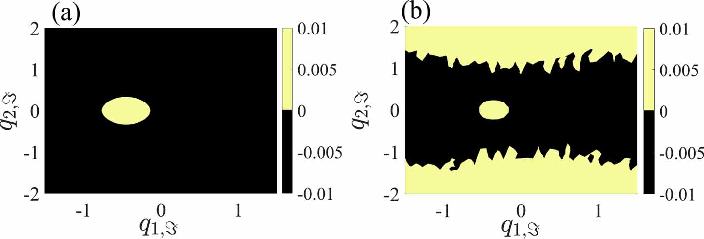
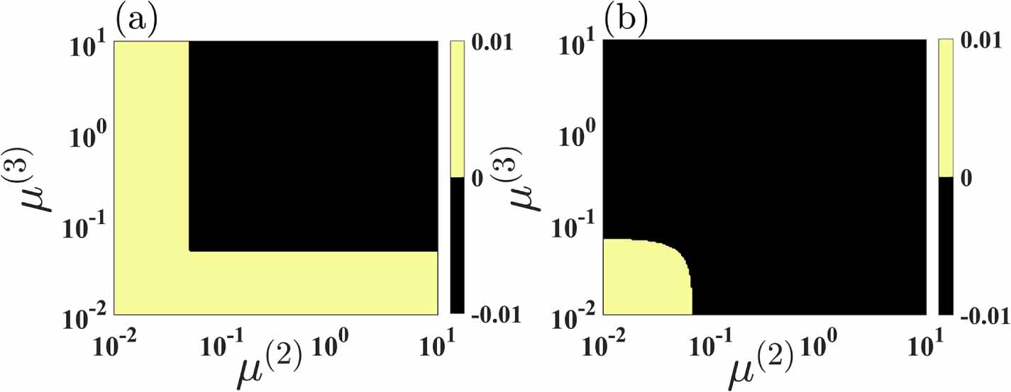
and  give the dynamics of transverse modes to the synchronization manifold. Hence the MSF can be obtained by solving equation (26) and provides the conditions for a global stable synchronous solution to exist. In figure 7, we show the level sets of the MSF as a function of the eigenvalues
  and
and  while keeping the remaining parameters in equation (26) fixed at generic nominal values. In panel (a), we consider a static hypergraph, i.e.
  , while in panel (b) a time-varying hypergraph, i.e.
  , negative values of MSF are reported in black and they correspond thus to a global synchronous state, positive values of MSF are shown in yellow. One can clearly appreciate that in the case of time-varying hypergraph, the MSF is negative for a much larger set of eigenvalues
  and
and  and thus the SL system can easily synchronize.

Figure 7. Synchronization on time-varying higher-order network of coupled SL oscillators with diffusive-like natural coupling. We report the MSF as a function of the eigenvalues  and
and  for two different choices of Ω,
  (panel (a)) and
  (panel (b)) by using a color code, black is associated to negative values while positive ones are shown in yellow. We characterize the range of the axes by considering the absolute values of the eigenvalues. The remaining parameters are kept fixed at
  ,
,  .
.
Download figure:
Standard image High-resolution image4. Synchronization of Lorenz systems nonlinearly coupled via time-varying higher-order networks
The aim of this section is to show that the previously presented results hold true beyond the example of the dynamical system shown above, i.e. the SL. We thus decide to propose an application of synchronization for chaotic systems on a time-varying higher-order network. For the sake of definitiveness, we used the paradigmatic chaotic Lorenz model for the evolution of individual nonlinear oscillators.
We consider again the scenario of regular topology with the toy model hypergraph structure composed of n = 4 nodes, 5 links and two three-hyperedges, i.e. triangular faces previously described. Moreover for sake of definitiveness we assume the x-variables to be coupled via a three-body term through a cubic nonlinear function, while the y-variables are coupled by using the network structure, i.e. the links. The whole system can thus be described by

where the system parameters are kept fixed at  ,
,  ,
,  , for which individual nodes exhibits chaotic trajectory. The pairwise and higher-order structures are related to each other by
  , with
  (see appendix
Let us thus select as reference solution  a chaotic orbit of the isolated Lorenz model and consider, as previously done, the time evolution of a perturbation about such trajectory. Computations similar to those above reported, allow to obtain a linear non-autonomous system ruling the evolution of the perturbation, whose stability can be numerically inferred by computing the MLE, i.e. the MSF. We first considered the impact of the coupling strength, ε1 and ε2 on synchronization by varying them freely over the range
 ![$[0,1.5]$](https://content.cld.iop.org/journals/2632-072X/5/1/015020/revision3/jpcomplexad3262ieqn250.gif) and
and ![$[0,0.04]$](https://content.cld.iop.org/journals/2632-072X/5/1/015020/revision3/jpcomplexad3262ieqn251.gif) . Here we vary the three-body coupling small only within a smaller region as the system becomes unbounded in presence of strong higher-order interactions. The corresponding results are reported in figure 8 where we present the level sets of the MSF as a function of the above parameters by using a color code: black dots refer to negative MSF while yellow dots to positive MSF. Panel (a) refers to a static hypergraph, i.e.
. Here we vary the three-body coupling small only within a smaller region as the system becomes unbounded in presence of strong higher-order interactions. The corresponding results are reported in figure 8 where we present the level sets of the MSF as a function of the above parameters by using a color code: black dots refer to negative MSF while yellow dots to positive MSF. Panel (a) refers to a static hypergraph, i.e.  , while panel (b) to a time-varying one, i.e.
  , one can thus appreciate that the latter setting allows a negative MSF for a larger range of parameters ε1 and ε2 and hence we can conclude that time-varying hypergraph enhance synchronization also in the case of chaotic oscillators.

Figure 8. Synchronization on time-varying regular higher-order network of coupled Lorenz oscillators. We report the MSF as a function of the coupling strengths, ε1 and ε2, for two different values of Ω,  (panel (a)) and
  (panel (b)), by using a color code, where black dots stand for a negative MSF, i.e. global synchronization, while yellow dots for a positive MSF. The remaining parameters are kept fixed at
  ,
,  ,
,  .
.
Download figure:
Standard image High-resolution imageTo emphasize the proposed framework, we realized numerical simulations involving the Lorenz system coupled again with the simple four-nodes time-varying hypergraph. We chose the parameters  , while the other parameter values are provided in figure 8. The numerical results presented in figure 8 lead us to the following conclusion: the region associated to a positive MSF, i.e. desynchronization of the Lorenz system, is larger in the case
  than for
  . Consequently, the system is much prone to achieve global synchronization on the time-varying hypergraph then in the static case. In figure 9 we report the evolution of the x-variable for each nodes as a function of time, such results corroborate the previous claim. In particular, in the case where
  (figure 9(b)), we observe that the x-variable shown phase coherence across all nodes, whereas such regular behavior is not present for
  , where the system does not any longer present an oscillatory behavior (figure 9(a)).

Figure 9. Time series of the signal xi
for a suitable choice of coupling parameters  and
and  . In panel (a), we set
  while
while  in panel (b). The other parameters values are the same as in figure 8, i.e.
  ,
,  ,
,  ,
,  .
.
Download figure:
Standard image High-resolution imageWe conclude this analysis by studying again the relation between the frequency Ω and the size of the coupling parameters ε1, ε2 on the onset of synchronization. In figure 10 we show the MSF in the plane  for a fixed value of
  (panel (a)), and in the plane
  for a fixed value of
  (panel (b)). By using again
  , for fixed ε2, and similarly
  , we can conclude that
  and
and  and thus supporting again our claim that time-varying structures allow to achieve synchronization easier.

Figure 10. We show the MSF in the plane  (panel (a)) for
  ) and in the plane
  (panel (b)) for
  ). We can observe that in both panels the critical value of coupling strengths
  to achieve synchronization is smaller for
  than for
  . This implies that synchronization can occur more easily on a time-varying higher-order structure than on a static one.
Download figure:
Standard image High-resolution image5. Conclusions
To sum up, we have here introduced and studied a generalized framework for the emergence of global synchronization on time-varying higher-order networks and developed a theory for its stability without imposing strong restrictions on the functional time evolution of the higher-order structure. We have demonstrated that the latter can be examined by extending the MSF technique to the novel framework for specific cases based either on the inter-node coupling scheme or on the topology of the higher-order structure. Our findings reveal that the behavior of the higher-order network is translated into an extra matrix term in the linearized system ruling the evolution of perturbation about the reference solutions; this matrix changes over time and possesses skew symmetry. This matrix is derived from the time-dependent evolution of the eigenvectors of the higher-order Laplacian. Additionally, the eigenvalues associated with these eigenvectors can also vary over time and have an impact on shaping the evolution of the introduced disturbance. We have validated the proposed theory on time-varying hypergraphs of coupled SL oscillators and chaotic Lorenz systems, and the results obtained indicate that incorporating temporal aspects into group interactions can facilitate synchronization in higher-order networks compared to static ones.
The framework and concepts presented in this study create opportunities for future research on the impact of temporality in systems where time-varying group interactions have been observed but not yet thoroughly explored due to the absence of a suitable mathematical setting. Importantly, the fact that our theory does not require any restrictions on the time evolution of the underline structure could offer the possibility to apply it for a diverse range of applications other than synchronization.
Data availability statement
The codes used in the simulations for this article is available openly on Github repository [43]. All other data that support the findings of this study are included within the article.
Appendix A: Non-invasive couplings
Here we will discuss the results corresponding to a slightly more general hypothesis for  , namely to be non-invasive, i.e.

whose goal is again to guarantee that the coupling term in equation (3) vanishes once evaluated on the orbit  . Indeed by using again
  and expanding equation (3) up to the first order we get

from equation (A.1) we can obtain

and thus rewrite (A.2) as follows

Recalling the definition of  given in equation (6) we get

By using the definition of the higher-order Laplace matrix (7) we eventually obtain

Let us consider now a particular case of non-invasive function, we assume thus there exists a function  , such that
  and define

then

where  is the Jacobian of the function
  evaluated at 0. In conclusion (A.5) rewrites as follows

where  can be considered as an effective time-varying simplicial complex or hypergraph.
Let us now observe that the effective matrix  is a Laplace matrix; it is non-positive definite (as each one of the
  does for any
  and any t > 0), it admits
  as eigenvalue associated to the eigenvector
  and it is symmetric. So there exist a orthonormal time-varying eigenbasis,
  ,
,  , for
, for  with associated eigenvalues
  . Similar to before, we define the n × n time dependent matrix
  that quantifies the projections of the time derivatives of the eigenvectors onto the independent eigendirections, namely

By recalling the orthonormality condition  we can again straightforwardly conclude that c is a real skew-symmetric matrix with a null first row and first column, i.e.
  and
and  .
.
Thereafter, we consider equation (A.7), and we project it onto the eigendirections, namely we introduce  and recalling the definition of c we obtain

This is the required master stability function, from which we can obtain conditions for stability of the synchronous solution.
A.1. Synchronization of Stuart–Landau oscillators with non-invasive coupling assumption
To validate the above results we again consider the SL oscillator with a particular case of non-invasive coupling function, namely we assume to exist a real function ϕ such that  ,
,  and
and

By reasoning as before, we get

By using again the eigenvectors  , eigenvalues
  of
of  and the matrix c (see equation (A.8)), we can rewrite the previous formula as

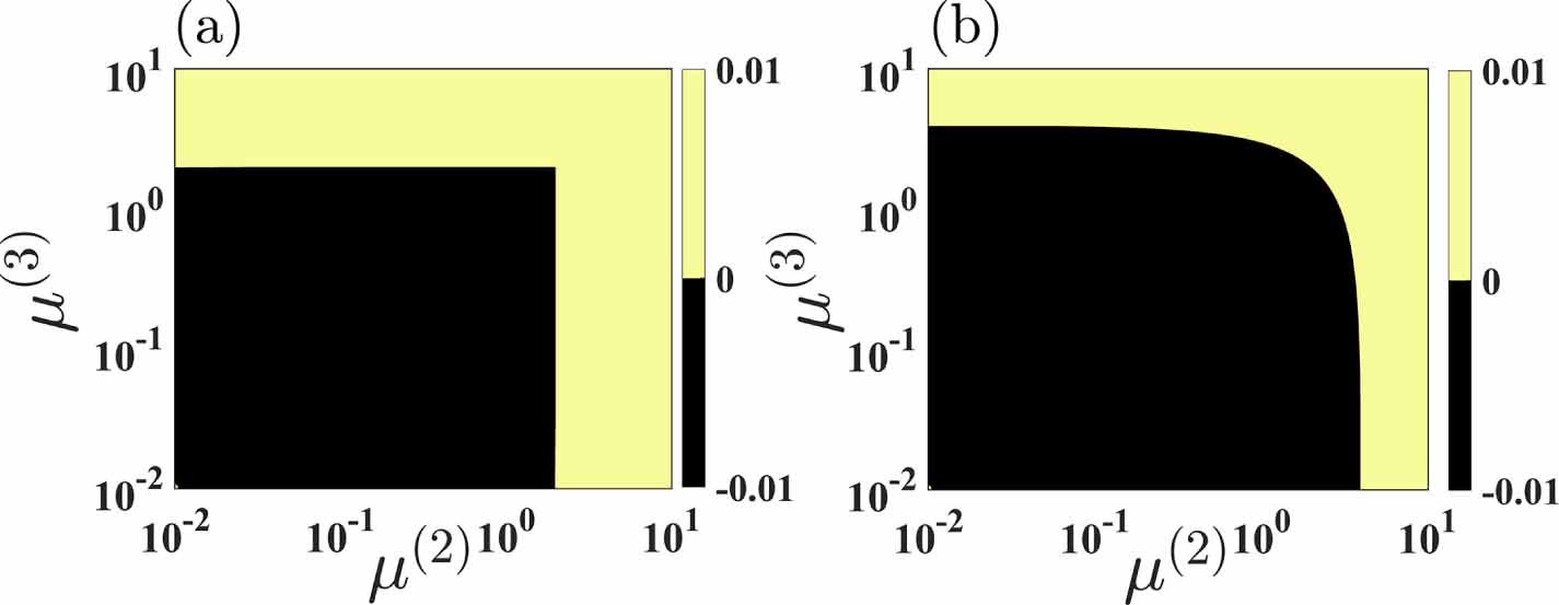
Figure A1 represent the result for the non-invasive coupling assumption. Here, we consider the non-invasive function so that  and the skew-symmetric projection matrix c is considered constant throughout the analysis as earlier. Here we show the level sets of the MSF as a function of the eigenvalues
  and
and  while keeping the remaining parameters in equation (A.12) fixed at generic nominal values. In panel (a), we consider a static hypergraph, i.e.
  , while in the (b) panel, a time-varying hypergraph, i.e.
  , negative values of MSF are reported in black, and they correspond thus to a global synchronous state, positive values of MSF are shown in yellow; one can clearly appreciate that in the case of the time-varying hypergraph, the MSF is negative for a much larger set of eigenvalues
  and
and  and thus the SL system can achieve synchronization more easily.

Figure A1. Synchronization on time-varying higher-order network of coupled SL oscillators with non-invasive coupling configuration. Region of synchrony and desynchrony are depicted by simultaneously varying  and
and  for two different values of Ω (a)
  , (b)
, (b)  , where the domain in black indicates the area of the stable synchronous solution. The range of the axes is characterized by considering the absolute values of the eigenvalues. All the other values are kept fixed at
  ,
,  ,
,  .
.
Download figure:
Standard image High-resolution imageAppendix B: Construction of the toy example hypergraph
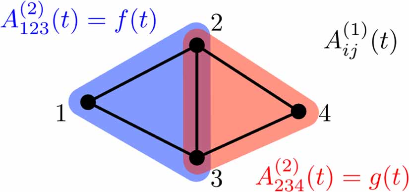
The goal of this section is to provide the details about the construction of the simple time-varying hypergraph exhibiting a regular structure and used in the main text. Let us thus consider thus an hypergraph composed by n = 4 nodes shared among two three-hyperedges whose 'weight' varies in time; consider also the existence of four edges, also depending on time. More precisely let us assume the three-tensor encoding the three-hyperedges are given by

where f(t) and g(t) are generic positive smooth functions and  denotes any permutation of the indexes ijk (see figure B1). Whereas, Whereas the weighted adjacency matrix describing the pairwise interactions, is assumed to be given by

By using the definitions equations (5) and (6) in the main text we can straightforwardly compute

hence the second order Laplace matrix (see equation (7) in the main text) is given by

From equation (B.2) it is straightforward to obtain the following Laplace matrix

and thus conclude that

namely the hypergraph shown in figure B1 is a regular structure. Let us observe that if we consider the same structure but with unitary weights, i.e. by assuming a binary adjacency matrix and a binary three-tensor, then the resulting static hypergraph will not be a regular structure. Indeed we can easily compute

(a simpler hypergraph would be trivial).
Remark Let us observe that the previous example is in some sense the smallest non trivial hypergraph one can construct with the above property. Indeed if we assume to have only n = 3 nodes and a single hyperedge, namely  , then we will obtain

whose associated two-Laplace matrix is

where in the last step we emphasized that the two-Laplace matrix is the product of a scalar function times a constant matrix. In this case the time dependence can be factored out and the analysis will be very similar to the case of constant hypergraph.

Figure B1. A simple time-varying hypergraph composed by n = 4 nodes, two three-hyperedges (represented by the red and blue triangles) and five links (represented by the black lines).
Download figure:
Standard image High-resolution imageB.1. Computing the spectrum of the time-varying three-hypergraph
The aim of this section is to compute explicitly the spectrum of the toy example hypergraph presented in the previous section. By using a symbolic manipulator one can easily compute the eigenvalues and eigenvectors of the three-hypergraphs and thus obtain

and

Let us observe that to increase the readability of the previous equation we did not explicitly wrote the normalizing factor s3 (resp. s4 ) for  (resp.
  ). One can easily show that eigenvalues and eigenvectors are real for all possible functions f(t) and g(t), and to prove that they are orthonormal and thus they form a basis for
  for all t.
A lengthy but straightforward calculation allows to obtain the matrix b (see equation (17) in the main text) that describes the evolution of the derivatives of the eigenvectors on the eigenbasis. Because of the form of the latter ones, we can show that all the entries of b are zero but  that is given by

where

and

where for ease of reading we removed the explicit dependence on t and ' denotes the first derivative with respect to t.
The numerical studies performed in the main text has been realized by assuming ![$f(t) = 1+[\sin(\Omega t)]^2$](https://content.cld.iop.org/journals/2632-072X/5/1/015020/revision3/jpcomplexad3262ieqn335.gif) and
and ![$g(t) = 1+[\cos(\Omega t)]^2$](https://content.cld.iop.org/journals/2632-072X/5/1/015020/revision3/jpcomplexad3262ieqn336.gif) , in this case the eigenvalues read
, in this case the eigenvalues read

and the non-zero element of the matrix b is

where ![$\tilde{N}_{34} = 24 \Omega \sin (2 t \Omega ) [\cos (2 t \Omega )+3]$](https://content.cld.iop.org/journals/2632-072X/5/1/015020/revision3/jpcomplexad3262ieqn337.gif) and
and ![$\tilde{N}_{34} = 2 \sqrt{2} [\cos (2 t \Omega )+3] [4 \cos (4 t \Omega )+13]$](https://content.cld.iop.org/journals/2632-072X/5/1/015020/revision3/jpcomplexad3262ieqn338.gif) .
.
Figure B2 portrays the temporal evolution of the links and three-hyperedges weights. To better understand the evolution of the hypergraph, we provide the graphical evolution of the hypergraph in the accompanying supplementary movie, together with the time evolution of the weights of the links  and of the hyperedge
  .
.

Figure B2. Temporal evolution of edges and three-hyperedge obtained for a particular value of  .
.
Download figure:
Standard image High-resolution image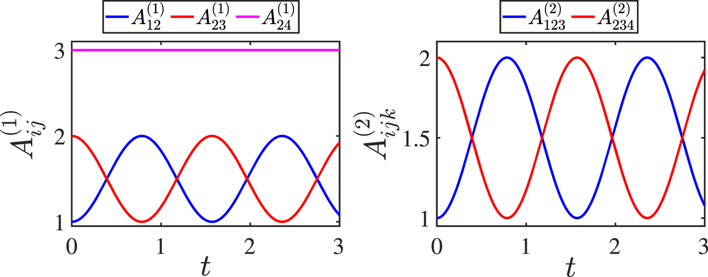