

Abstract
Spatial climate analogs effectively illustrate how a location's climate may become more similar to that of other locations from the historical period to future projections. Also, novel climates (emerging climate conditions significantly different from the past) have been analyzed as they may result in significant and unprecedented ecological and socioeconomic impacts. This study analyzes historical to future spatial climate analogs across East Asia and Europe, in the context of climatic impacts on ecology and human health, respectively. Firstly, the results of climate analogs analysis for ecological impacts indicate that major cities in East Asia and Europe have generally experienced novel climates and climate shifts originating from southern/warmer regions from the early 20th century to the current period, primarily attributed to extensive warming. In future projections, individual cities are not expected to experience additional significant climate change under a 1.5 °C global warming (warming relative to pre-industrial period), compared to the contemporary climate. In contrast, robust local climate change and climate shifts from southern/warmer regions are expected at 2.0 °C and 3.0 °C global warming levels. Specially, under the 3.0 °C global warming, unprecedented (newly emerging) climate analogs are expected to appear in a few major cities. The climate analog of future projections partially align with growing season length projections, demonstrating important implications on ecosystems. Human health-relevant climate analogs exhibit qualitatively similar results from the historical period to future projections, suggesting an increasing risk of climate-driven impacts on human health. However, distinctions emerge in the specifics of the climate analogs analysis results concerning ecology and human health, emphasizing the importance of considering appropriate climate variables corresponding to the impacts of climate change. Our results of climate analogs present extensive information of climate change signals and spatiotemporal trajectories, which provide important indicators for developing appropriate adaptaion plans as the planet warms.
Export citation and abstract BibTeX RIS

Original content from this work may be used under the terms of the Creative Commons Attribution 4.0 license. Any further distribution of this work must maintain attribution to the author(s) and the title of the work, journal citation and DOI.
1. Introduction
Anthropogenic greenhouse gas emissions have caused global-average and local warming, and global-average precipitation increase (IPCC 2021), although precipitation changes have been spatially heterogeneous (Gulev et al 2021). Observed temperature and precipitation changes are projected to continue during the 21st century contingent upon the continuation of greenhouse gas emissions (Lee et al 2021).
In the context of climate change, analogous conditions to the climate of a specific location of interest are referred to as climate analogs (Mahony et al 2017). Climate analog mapping illustrates matching climate shifts from another potentially familiar location and provides a more relatable, place-based, and intuitive assessment of climate change. Climate analogs analysis that consider various climate variables (e.g. temperature, precipitation) have been utilized to illustrate novel climates (emerging climates with no analogs in the past) in a location, climate shifts between different locations during the historical period (Abatzoglou et al 2020, King 2023) and future projections (e.g. Mahony et al 2017, Bastin et al 2019, Fitzpatrick and Dunn 2019, Nguyen-Thi et al 2021). Climate analog analysis is straightforward and informative for several climate-relevant socioeconomic perspectives, including human health (Kalkstein and Greene 1997, Fischer and Knutti 2013), agriculture (Webb et al 2013), ecosystems (Burke et al 2019, Holsinger et al 2019, Thompson and Fronhofer 2019, Pandolfi et al 2020, Dobrowski et al 2021) and reforestation decisions (MacKenzie and Mahony 2021) depending on the climate variables considered in computing the analogs.
Previous climate analog analyses have focused on future projections relative to current conditions. This has included studies on climate shifts to warmer and drier conditions in cities from the Northern Hemisphere and tropics, respectively, by 2050 (Bastin et al 2019), extensive emergence of climate novelty/shifts across North America (Mahony et al 2017, Fitzpatrick and Dunn 2019), climatic relocation towards warmer regions for the five big cities in Southeast Asia (Nguyen-Thi et al 2021), and emergence of novel climates/climate analog shifts in China (Yin et al 2020). Based on regional climate model simulations under the emission scenarios of the Special Report on Emissions Scenarios (Nakićenović et al 2000), Rohat et al (2018) projected a north-to-south transect-oriented shift in the climate of European cities during specific future periods (e.g. 2071–2100), based on simple averaged Euclidean distances of climate variables between future and current climates. Based on the Köppen climate classification, over Europe, Jylhä et al (2010) reported climatic zones shifting toward a warmer or drier climate type during the historical period (from the mid-20th century) to future projections based on observations and coupled model intercomparison project (CMIP) phase 3 (CMIP3; Meehl et al 2007) multi-model simulations. Lotterhos et al (2021) observed a weak climate change signal over the global surface ocean environment during the historical period, while a large portion of the global surface ocean is expected to encounter climate novelty and global disappearance in the future, indicating that the future climate conditions will fall outside the present day climate envelope for the globe. Regarding climate extremes, Sano and Oki (2022) showed that many people will be exposed to extreme climatic (extreme temperature and precipitation) risks in the future along with the emergence of unfamiliar climatic risks in several regions; Wang et al (2023) presented the movement of best analogs for extreme temperature and precipitation in China cities to contemporary regions exhibiting intense heat and extreme precipitation, respectively, under 2.0 °C global warming.
Although there has been a lot of research, prior analyses of historical climate analogs have been limited, especially regarding how climate shifts between different locations (e.g. King 2023). Extensive analyses of extratropical Eurasia, such as East Asia and Europe have not been conducted until now for both historical (from the early 20th century to the current period) and future projections by employing the latest coupled climate model simulations (i.e. CMIP6; Eyring et al 2016). Furthermore, it is essential to consider specific global warming levels, including those referred to the Paris Agreement. In the context of implications arising from climate shift/novelty, the consideration and inter-comparison of various climate envelopes are crucial in climate analogs analysis. Applying the improved statistical methodology suggested by Mahony et al (2017) would be effective in these analyses. To advance further while addressing these limitations, we conducted climate analogs analysis over East Asia and Europe capital/major cities, where many people live, but have not been systemetically analyzed in previous studies. Two climate analogs with potential implications on ecology and human health were considered, respectively, adopting an improved analysis framework. Using observations, we examined the climate novelty and spatial movement of climate analogs from the early 20th century to the present. Moreover, we explored future projections of spatial climate analogs under specific global warming levels to identify novel climates and the best historical analogs for each location's future climate. Understanding the continuum of climate analogs from the past to future projections would be beneficial for extensively comprehending the historical and future climate change in a city, compared to analyzing them separately. Also, the results of climate analogs analysis can be used to intuitively communicate historical and future climate changes. Despite the limited utilization of climate analogs in communicating the impacts of climate change thus far, it is imperative to exercise caution in presenting these findings to diverse audiences (Retchless 2014).
2. Data and methods
2.1. Observations
Observational datasets from version 4 of the Climatic Research Unit gridded time series (CRU TS v4; Harris et al 2020) were used in this study. Gridded datasets of monthly mean daily maximum and minimum near-surface temperatures, as well as precipitation, spanning from 1901 to 2021, were acquired. These datasets feature a horizontal resolution of 0.5° × 0.5° and cover global land areas. The datasets were produced through the interpolation of extensive networks of weather station observations. Sensitivity tests were conducted by employing Berkeley Earth Surface Temperature (BEST; Rohde et al 2013) and Global Precipitation Climatology Centre (GPCC; Schneider et al 2022) datasets. These tests, conducted at a horizontal resolution of 1.0° × 1.0°, aimed to validate the robustness of our findings. For surface relative humidity, we utilized European Centre for Medium-Range Weather Forecasts reanalysis version 5 (ERA5; Hersbach et al 2020) dataset.
2.2. CMIP6 model simulations
The CMIP6 multi-model ensemble of coupled climate simulations (Eyring et al 2016) were used in this study. The NASA Earth Exchange Global Daily Downscaled Projections (NEX-GDDP-CMIP6; Thrasher et al 2022) datasets were used to conduct spatial climate analog analysis under fine horizontal resolution. These datasets provide statistically bias-corrected and downscaled CMIP6 model simulations over global land at a horizontal resolution of 0.25° × 0.25°. The datasets were produced through quantile mapping bias-correction and spatial disaggregation, where temporal fluctuations are interpolated and added/multiplied to observed historical climatology (see details in Thrasher et al 2022). All available model simulations (27 models, one ensemble per each model; table S1) were used, which provide all analyzed variables in this study for historical simulations (forced with both anthropogenic and natural external forcings; 1950–2014) and high-emission scenario (Shared Socioeconomic Pathway (SSP) 5–8.5; O'Neill et al 2016) experiments (2015–2100).
2.3. Cities and climate variables
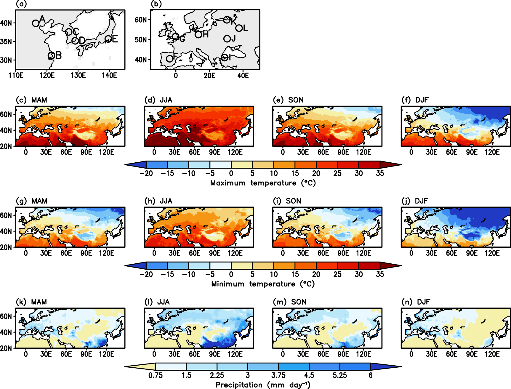
We analyzed climate analogs in five and seven cities over East Asia and Europe, respectively (see figures 1(a) and (b)). In East Asia, five cities–Seoul, Busan, Shanghai, Beijing and Tokyo–were selected due to their the first or second largest number of population in South Korea, China, and Japan. Furthermore, most of these cities hold high rankings in East Asia in terms of resident population. In Europe, seven cities–Berlin, Istanbul, Kyiv, London, Madrid, Moscow and Saint Petersburg were chosed, where the largest number of populations are living.

Figure 1. (a), (b) Location of cities analyzed for climate analogs are denoted by black circles on regional maps, across (a) East Asia ('A' for Beijing, 'B' for Shanghai, 'C' for Seoul, 'D' for Busan, and 'E' for Tokyo) and (b) Europe ('F' for Madrid, 'G' for London, 'H' for Berlin, 'I' for Istanbul, 'J' for Kyiv, 'K' for Saint Petersburg, and 'L' for Moscow). (c)–(n) Spatial patterns of seasonal mean (c)–(f) maximum temperature, (g)–(j) minimum temperature, and (k)–(n) precipitation climatology during 2000–2019/20 for (c), (g), (k) March–May (MAM), (d), (h), (l) June–August (JJA), (e), (i), (m) September–November (SON), and (f), (j), (n) December–February of the following year (DJF).
Download figure:
Standard image High-resolution imageIn first, in the context of ecological impacts, climate analogs analysis involves utilizing the seasonal average daily maximum and minimum temperatures along with precipitation (cube root transformation is applied for seasonal mean precipitation to make distributions nearer normal; King 2023) during the four meteorological seasons (March–May (MAM; boreal spring), June–August (JJA; boreal summer), September–November (SON; boreal autumn) and December to February of the following year (DJF; boreal winter)) in each city. This climate envelope holds broad implications for ecosystems (Williams et al 2007, Mahony et al 2017). Figures 1(c)–(n) present the climatology of the variables in each season over extratropical Eurasia and individual cities' seasonal cycles are presented in figure S1. Climatology from BEST and GPCC are presented in figure S2, which exhibits extremely consistent spatial values with CRU TS v4 (figures 1(c)–(n)), demonstrating minimal observation uncertainty in terms of climatological values. Furthermore, for the analysis of climate analogs in terms of human health impact (section 3.4), we examined surface relative humidity instead of cube-rooted precipitation, as a combination of temperature and relative humidity has been used to define wet-bulb globe temperature (Fischer and Knutti 2013, Lee and Min 2018).
2.4. Climate analogs analysis
We conducted a climate analog analysis to identify locations with similar climates during the early 20th/mid-20th century and the current period, serving as comparisons for each city's current and future climate, respectively. The analytical method developed by Mahony et al (2017) is used, which utilizes the Mahalanobis distance and the resultant sigma dissimilarity. For individual cities and a set of climate variables, we taked the following series of steps (Mahony et al 2017, Fitzpatrick and Dunn 2019, King 2023):
- 1.Each city's climate variable is standardized based on the recent 20 years (MAM 2000 to DJF 2019/20) mean and standard deviation (the latter is calculated after removing the linear trend) for each season. [C'] comprises a (T × K) matrix of detrended concurrent climate anomalies (20 years for T) of K climate variables (e.g. when considering the maximum and minimum temperatures along with precipitation for all four seasons, the value of K is found to be 12) at each city (see example in figure S3(a)).
- 2.Principal component (PC) analysis is performed on [C']. The maximum number of extracted PCs is the same as the number of variables (i.e. K) considered in this calculation. Retaining most or all the PCs is rational because we are interested in conserving the spatial variation and climate change signals in the datasets. We discarded PCs with explaining variances of less than 1% to mitigate the risk of artificially amplified spatial variation or climate change signals by standardization against trivial variance in climate variabilities, as recommended by Mahony et al (2017). Constructed PCs account covariance between the climate variables, which helps to investigate significance of results from independent samples (see below).
- 3.For individual locations (i.e. individual grids), all variables are averaged over 20 yr in the early 20th century (MAM 1901 to DJF 1920/1921), the mid-20th century (MAM 1950 to DJF 1969/70), and current period (MAM 2000 to DJF 2019/20) and standardized by using each city's mean and standard deviation calculated from the current period (MAM 2000 to DJF 2019/20, computed in step 1). Standardization was performed by utilizing the mean and standard deviation of the city of interest, which enables the evaluating the degree to which the climate of each grid resembles that of the specified city. The standardized values are compiled to [A'], which comprises (K) matrix of K climate variables' standardized 20 year averages for each period (early 20th century, mid-20th century, and current period) and each location for analyzing each city's climate analogs (see example in figures S3(b) and (c)).
- 4.For each city of interest, [B'] was compiled, including the standardized climatology of all analyzed variables relative to the mean and standard deviation of the current period (MAM 2000 to DJF 2019/20). This compilation is represented by the (K) matrix of K climate variables' standardized 20 year averages in each city. This process was conducted for the climatology of the current period (MAM 2000 to DJF 2019/20; i.e. standardized values are set to zero), and future projections (20 years under specific global warming levels, as detailed in section 3.2), which were undertaken to facilitate the spatial climate analogs analysis for the city's historical and future climates, respectively.
- 5.[A'] and [B'] are projected on PCs obtained in step 2. Subsequently, the Mahalanobis distance (
 ) was computed within the transformed datasets as follows:where is the location of each city, is any grid, is the number of PCs, is each PC projected onto [B'], is each PC projected onto [A'], and is the standard deviation of each PC projected onto [C']. It is reasonable to project [A'] and [B'] onto the PCs obtained from annual data, as our objective is to restore the anomalies while considering a city's intrinsic properties reflected in the constructed PCs. The magnitude of the differences in the projected outcomes between [A'] and [B'] may depend on absolute climate change signals.
 - 6.The sigma dissimilarity is computed by converting using the Chi-distribution, such that there may be comparability between locations where the value of is different. The use of the Chi-distribution in this analytical framework is justified, as it fundamentally characterizes the distribution of the square root of a sum of squared independent Gaussian variables, which is equivalent to the distribution of the Euclidean distance between a multivariate independent Gaussian variables. can be represented probabilistically as percentiles of the Chi-distribution. Translation of distances into probabilities is required to account for the effect of dimensionality on the statistical meaning of distance. Subsequently, these percentiles are expressed using the terminology of z-scores to estimate sigma dissimilatity. For instance, 1σ and 2σ are used to describe 68th and 95th normal percentiles, respectively. This sigma dissimilarity functions as a multivariate z-score metric, indicating the percentile of a given within the Chi-distribution. Values of sigma dissimilarity exceeding 8.21 proved challenging to estimate accurately, due to heightened decimal precision necessary for probability estimation in the extreme tail of the Chi-distribution, as mentioned by Lotterhos et al (2021). These instances are denoted as >8.21σ.


Each city is considered to transition to a novel climate when the sigma dissimilarity, between the city's own climates in different periods exceeds 2σ, as outlined by Mahony et al (2017). Furthermore, for individual cities and analysis periods, location of best analog is defined as the location with smallest sigma dissimilarity over the global land.
3. Results
3.1. Historical climate analogs
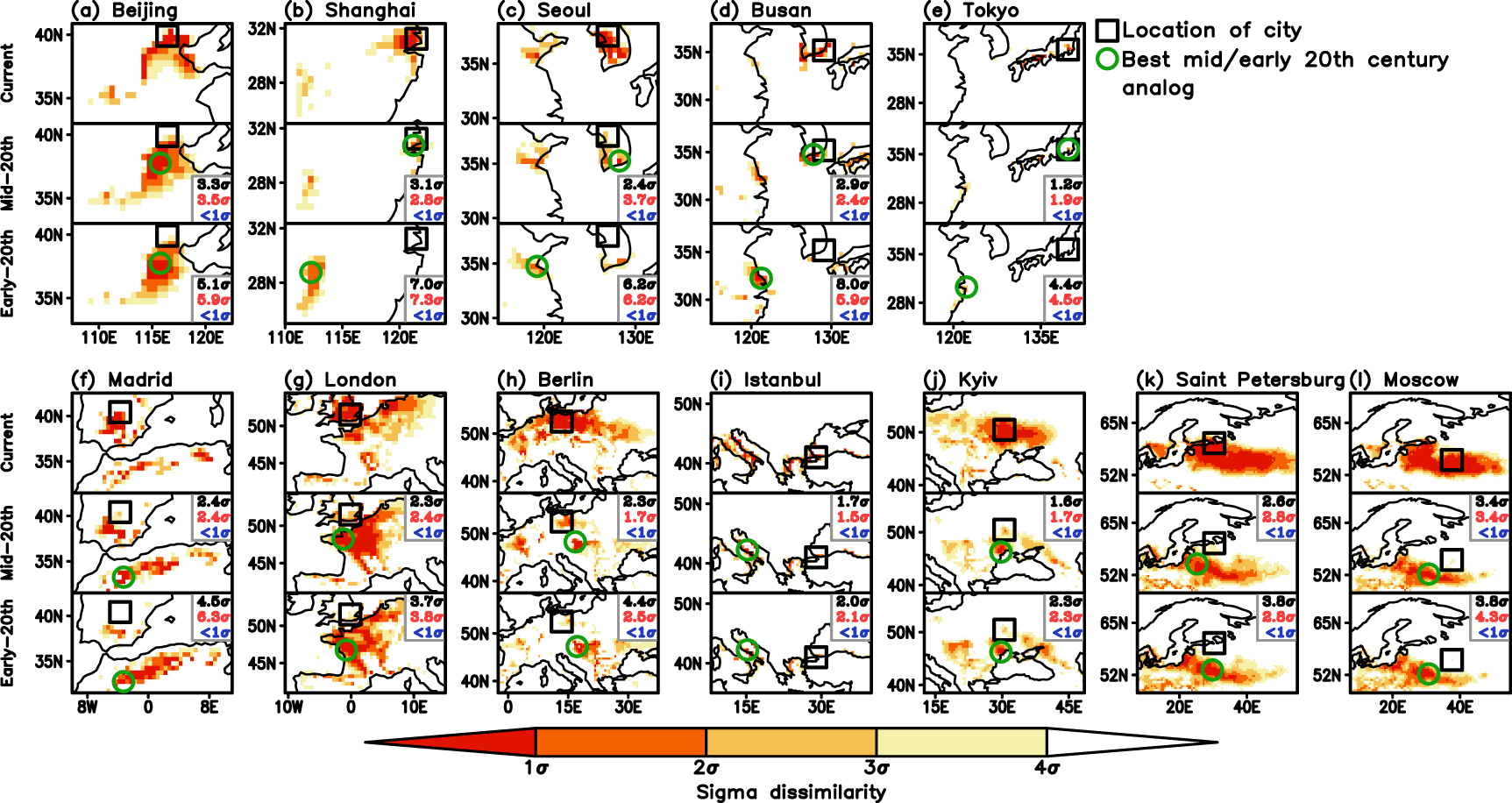
Figure 2 shows spatial climate analogs analysis results over East Asia and Europe during the historical period. Sigma dissimilarity values were calculated between each city location's current climate (2000–2019/20) and the climate at all locations during the current period, mid-20th century (1950–1969/70), and early 20th century (1901–1920/21). Most cities have experienced novel climates at their location since mid-20th century, with the exceptions of Tokyo, Istanbul and Kyiv (1.2σ–1.7σ). Notably, cities have experienced much greater climate change from the early 20th century to the present (>2σ in all cities except for Istanbul), demonstrating a robust experience of climate changes from the 20th to the early 21st century, primarily driven by alterations in local seasonal maximum and minimum temperature, while precipitation variations did not contribute greatly (figure 2, comparing black, red and blue sigma dissimilarity values). It is noteworthy that the sigma dissimilarity values from considering both temperatures and precipitation, may not exhibit a strictly linear pattern compared to analyses solely focused on temperatures (e.g. in comparison of mid-20th century results between Tokyo, Berlin and Istanbul). Despite the significant influence of temperature changes on the climate analogs, the combined consideration of temperatures and precipitation introduces complexities into the analysis procedures (e.g. [C'], PCs, and number of PCs in use) that may not align with a straightforward linear representation of sigma dissimilarity values. The observed climate changes vary across regions, with cities in East Asia tend to have experienced greater changes than Europe, which can be attributed, in part, to smaller inter-annual temperature variabilities in the East Asian regions (figure S4). The best analogs during the mid-20th century corresponding to current climates of cities were generally located in the southern/warmer regions from the location of the cities, and generally located even further southern/warmer regions, during the early 20th century, representing a progressive movement of climate analogs during the historical periods (e.g. current climate of Seoul mostly resembles that of the mid-20th century in Jinju (South Korean city) and early 20th century in Lianyungang (Chinese city)). Spatial patterns of sigma dissimilarity relative to the best analogs, demonstrate greater similarity in the vicinity of the best analogs, as would be expected (figure S5). The findings illustrated in figure 2 consistently persist when we replicated our analysis by incorporating extended years for both the early 20th and mid-20th century periods (figure S6).

Figure 2. Sigma dissimilarity values between the city's current (2000–2019/20) climate and climates in other locations during the current period (2000–2019/20; top), mid-20th century (1950–1969/70; middle), and early 20th century (1901–1920/21; bottom). Sigma dissimilarity between the periods at each city's location is given in the (a)–(e) bottom-right, (f)–(l) top-right of each map (enclosed by gray lines) based on the city's climate envelope (temperatures and precipitation; black), temperatures alone (red), and precipitation alone (blue) (only shown at middle and bottom panels in each figure). Black squares and green circles indicate the city's location and best analog in each period, respectively (green circles apprear only in the middle and bottom panels of each figure).
Download figure:
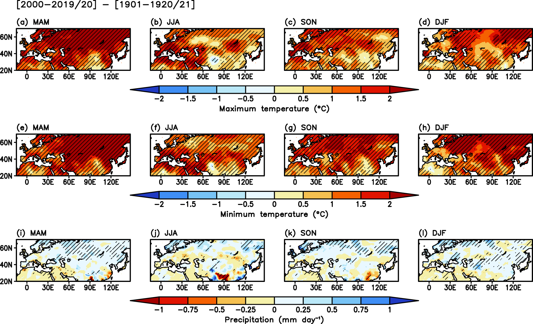
Standard image High-resolution imageFigure 3 illustrates the spatial patterns of historical change (2000–2019/20 minus 1901–1920/21) for maximum and minimum temperatures and precipitation, which shows robust warming trend across all seasons during the historical period, whereas precipitation changes exhibit greater diversity and insignificance. These have resulted in historical warming-driven local climate change and spatial movement of climates (figure 2). In addition, repeating our analysis based solely on seasonal average maximum and minimum temperatures (figure S7) and only on precipitation (figure S8) proves that the movement of the best climate analogs are primarily attributed to historical temperature warming. Notably, extensive regions tend to exhibit similar precipitation-based sigma dissimilarity values owing to large precipitation variability (figure S8), which complicates the detection of a clear precipitation signal. It is noteworthy that there is potential uncertainty in observation datasets depending on the methdology used to construct the datasets (e.g. interpolation). In terms of the possible uncertainty in the observation datasets, robustness of our results were confirmed when we repeated the analysis using BEST and GPCC (figure S9).

Figure 3. Spatial patterns of historical changes (2000–2019/20 relative to 1901–1920/21) in seasonal mean (a)–(d) maximum temperature, (e)–(h) minimum temperature, and (i)–(l) precipitation for (a), (e), (i) March–May (MAM), (b), (f), (j) June–August (JJA), (c), (g), (k) September–November (SON), and (d), (h), (l) December–February of the following year (DJF). Hatchings indicate regions with significant change at a 5% level based on Student's t-test.
Download figure:
Standard image High-resolution image3.2. Future projection of climate analogs
In this section, we examined contemporary climate analogs of the future climate of indiviudal cities using NEX-GDDP-CMIP6 multi-model simulations (section 2.2). First, we evaluated the performance of the model simulations to identify the applicability of the spatial climate analog analysis. The results of the analysis in the historical period (figure S10; using model simulation [C'] and PCs, and projecting observed [A'] and [B']) generally present similar results to the observations (figure 2) but with a few limitations (e.g. Seoul, figure S10(c)). To avoid these biases, we adopted observation [C'] and PCs, and projected model simulations' [A'] and [B'] (standardized with respect to 2000–2019/20 mean and standard deviation) to the PCs in future projection analysis. This analysis strategy is rational because the NEX-GDDP-CMIP6 simulations are observationally bias-corrected downscaled datasets (Thrasher et al 2022; overall spatial patterns of climate variables are relatively consistent with observations; section 2.2), and the analyses are based on standardized climate variables.
From the CMIP6 historical (1850–2014) merged with high-emission scenario (SSP5-8.5; 2015–2100; O'Neill et al 2016) simulations, we selected a 20 year period, when their averages are mostly close to 1.5, 2.0, and 3.0 °C global warming levels relative to the pre-industrial period (1850–1900 average) in each CMIP6 model simulation (figure S11). Figure 4 presents the result of spatial climate analogs analysis in future projections through estimating sigma dissimilarity values between each city location's climate under 1.5, 2.0, and 3.0 °C global warming levels and current climates of all locations (2000–2019/20, historical and SSP5-8.5 simulations were merged). First, the results indicate a notable absence of significant local climate change under a 1.5 °C global warming level when compared to the current period, particularly in cities across Europe (top panel of figure 4; with high inter-model agreement), possibly due to the relatively modest additional warming between the periods (figure S11; i.e. 0.97 °C warming already evident in the CMIP6 multi-model simulations average in the current period compared to the pre-industrial period). These results demonstrate the avoidance of additional significant climate change in each city when warming stopped at the 1.5 °C global warming level. In contrast, pronounced climate changes emerge in the cities under 2.0 °C global warming, and the cities' future climate will resemble that of the southern/warmer regions' current climate (2000–2019/20), except for London and Istanbul (middle panel of figure 4).

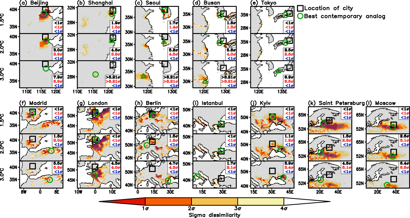
Figure 4. NEX-GDDP-CMIP6 multi-model median sigma dissimilarity between each city's climate under the (top) 1.5 °C, (middle) 2.0 °C, and (bottom) 3.0 °C global warming and other location's current (2000–2019/20) climate. Sigma dissimilarity values for each city's location are provided in the (a)–(e) bottom-right, (f)–(l) top-right of each map (enclosed by gray lines), based on the city's climate envelope (temperatures and precipitation; black), temperatures alone (red), and precipitation alone (blue). Black squares indicate individual cities' locations. Green circles (triangles) denote the best contemporary climate analog in each period where the multi-model median and more than 70% of model simulations consistently (inconsistently) present smaller or greater 2σ dissimilarities. Blue and gray hatchings indicate regions where multi-model median and more than 70% of model simulations display smaller and greater 2σ dissimilarities, respectively.
Download figure:
Standard image High-resolution imageDuring the 20 yr period when global warming reaches 3.0 °C relative to the pre-industrial period, all analyzed cities are projected to experience robust climate changes, mostly beyond 4σ dissimilarity (bottom panel of figure 4), indicating the requirement for intense adaptation. Remarkably, the spatial distribution of contemporary climate analogs in future projections under additional warming for individual cities (figure 4) exhibit a general similarity to the climate analogs observed in the early 20th/mid-20th century corresponding to the current climate (figure 2). This implies that referencing the directional trends of climate shifts during the historical period may consistently reappear in the future. Furthermore, referencing specific regional climates can be a useful approach for understanding the future climate in a corresponding city under continuous warming. However, it is noteworthy that the sigma dissimilarity at best analogs of Beijing and Shanghai under 3.0 °C global warming level is 5.1σ and 2.8σ, respectively, indicating these cities will experience newly emerging climates–essentially unprecedented climates (i.e. even the location with the most similar current climate exhibits a strongly different climate to that of Beijing and Shanghai under a high global warming level). These results show an increased complexity compared to results specific to individual regions in demonstrating similar climates during the current period. This complexity is crucial for understanding possible ecoregions (i.e. habitats) movement necessary to track changing environments, as discussed by Dobrowski et al (2021).
The anticipated climate change for each city in the future primarily attributed to regional warming rather than precipitation changes, even under the 3.0 °C global warming (figure 4). However, it is important to note that, future significant precipitation changes are evident under continuous warming, as highlighted in the IPCC (2021).
3.3. Ecological implications of climate analogs
The results of the climate analogs in this study, encompassing the climate envelope of seasonal mean maximum and minimum temperatures and precipitation, likely hold broad ecological significance (Williams et al 2007, Mahony et al 2017). When considering plant growth, growing season length (GSL) serves as an important indicator, defined as the annual count between the first span of at least 6 d with daily mean surface air temperature >5 °C and the first span after 1st July of 6 d with daily mean surface air temperature <5 °C for the Northern Hemisphere (Peterson et al 2001). Historical records indicate an extension of the GSL during the historical period (Mueller et al 2015). Figure 5 presents future projections of GSL using NEX-GDDP-CMIP6 simulations, based on a comparable methodology to the prior spatial climate analogs analysis. These analogs are presented as sigma anomalies between each city's GSL in future projections (1.5, 2.0, and 3.0 °C global warming presented as a 20 yr average) and the GSL of other locations in the current period (2000–2019/20), standardized based on the city's standard deviation in the current period. The results reveal that, although each city's GSL projection generally does not exhibit significant changes up to 2.0 °C global warming, each city's future GSL will be similar to GSLs observed in southern/warmer locations (gray shadings, absolute differences smaller than 0.5σ) during the current period. Although not precisely identical, the regions displaying comparable GSL with future projections for the city of interest during the current period (figure 5) generally coincide with the ecology-relevant climate analogs in the current period that most closely resemble the city's future climate under specific warming levels presented, as illustrated in figure 4 (e.g. Busan, Moscow).
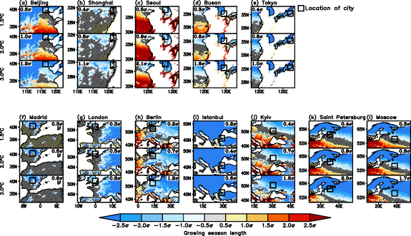
Figure 5. NEX-GDDP-CMIP6 multi-model median differences in standardized growing season length between each city's value under the (top) 1.5 °C, (middle) 2.0 °C, and (bottom) 3.0 °C global warming and the values of other locations during the current period (2000–2019/20) (values for the current period across all locations minus future projections specific to each city of interest; standardized based on city's standard deviation in the current period). Multi-model median projections at each city's location are given in (a)–(e) top-left, (f)–(l) top-right of each map. Black squares indicate individual cities' locations. Black hatchings indicate regions where the multi-model median and more than 70% of model simulations present results within the ±1σ range.
Download figure:
Standard image High-resolution image3.4. Human health-relevant climate analogs
The climate envelope used in our aforementioned findings is constructed based on seasonal mean maximum and minimum temperatures, along with precipitation, providing valuable insights into climate change impacts on ecology and socioeconomics. However, for a comprehensive understanding of human health implications, constructing climate envelopes using temperature and relative humidity, variables used for defining wet-bulb globe temperature (e.g. Fischer and Knutti 2013, Lee and Min 2018) would be beneficial. Here, we analyze climate analogs relevant to human health, specifically focusing on heat stress, using seasonal (boreal spring, summer and autumn) mean maximum and minimum temperatures (from CRU TS v4) and relative humidity at the surface (from ERA5). Boreal spring and autumn are jointly analyzed to consider extensive warm periods throughout the seasons in individual cities (see figure S1), which is suitable to consistently apply in both historical and future projection analyses, considering historical and anticipated future summer season lengthening (Park et al 2018, 2022).
The climate analogs analysis consistently reveals notable local climate changes and shifts originating from the southern/warmer regions during the historical period, mostly due to temperature increases (figure 6). One notable point is the significant influence of relative humidity changes on the climate change signals observed over Beijing, Shanghai, Tokyo and Saint Petersburg during the historical period, predominantly caused by the decreasing trend in relative humidity, particularly across the cities in East Asia, as depicted in figure S12 (also, suggested in Gulev et al 2021, IPCC 2021), which may partly offset the warming-induced increase in heat stress over the regions.

Figure 6. Same as the top and middle panels of figure 2, but climate analogs were based on seasonal mean maximum and minimum temperatures along with relative humidity during boreal spring, summer and autumn (three climate variables for three seasons). Sigma dissimilarity between the periods at each city's location is presented at the (a)–(e) bottom-right, (f)–(l) top-right of each map (enclosed by gray lines), based on the city's climate envelope (temperatures and relative humidity; black), temperatures alone (red), and relative humidity alone (blue) (only shown at below panel of each figure). (e) For Tokyo, best mid-20th century analog is not shown, which is located outside the displayed regions.
Download figure:
Standard image High-resolution imageFuture projections of human health-relevant climate analogs (figure 7) present results similar to figure 4 (i.e. ecology-relevant climate analogs); strong local climate changes mostly from 2.0 °C global warming and general climate analogs movement toward southern/warmer regions. However, the results indicate more pronounced local climate change signals in specific regions, such as Tokyo, London, and Moscow, along with different spatial patterns of sigma dissimilarity compared to future projections of ecologically relevant climate analogs (figure 4), highlighting the importance of constructing a climate envelope that corresponds to the impact of climate change. Furthermore, the sigma dissimilarity values for the best analogs of Beijing, Shanghai, Tokyo, and Saint Petersburg under a 3.0 °C global warming ranges from 2.5σ to 3.4σ, indicating these cities may undergo the emergence of new climates, potentially impacting human health.

Figure 7. Same as figure 4, but climate analogs were based on seasonal mean maximum and minimum temperatures along with relative humidity during boreal spring, summer and autumn (three climate variables for three seasons). Sigma dissimilarity between the periods at each city's location is displayed at the (a)–(e) bottom-right, (f)–(l) top-right of each map (enclosed by gray lines), based on the city's climate envelope (temperatures and relative humidity; black), temperatures alone (red), and relative humidity alone (blue).
Download figure:
Standard image High-resolution image
4. Discussion and conclusions
This study presents historical and future spatial climate analog analyses for East Asia and Europe. Climate envelopes were constructed to analyze spatial climate analogs, considering seasonal mean maximum and minimum temperatures, as well as precipitation or relative humidity. These analyses hold crucial implications for broad ecological systems, socioeconomic impacts, and human health.
Major cities within these areas have generally experienced significant climate changes during the historical period, primarily attributed to local warming under increasing greenhouse gas emissions. Besides that, during the historical period, changes in relative humidity were identified as contributors to climate change in Beijing, Shanghai, Tokyo, and Saint Petersburg, which partly offset warming-induced heat stress increases, particularly in cities across East Asia. Analysis of spatial climate analogs indicates a notable shift of climates during the historical period from the southern/warmer regions to individual cities with progressive movements from the early 20th and mid-20th centuries to the current periods. The spatial movements of climate analogs intricately linked to the pronounced historical warming across these regions.
The results of future climate analogs analysis generally present weak climate change signals in each location during the 20 years when experiencing 1.5 °C global warming (relative to pre-industrial period) compared to the current climate, illustrating the possibility for avoiding additional significant climate changes over the analyzed cities in East Asia and Europe by meeting the Paris Agreement goals. In contrast, at 2.0 °C global warming, each location's climate change signal and climate shifts became more pronounced, demonstrating the requirement of robust mitigation efforts to prevent greater warming. Under the 3.0 °C global warming, model simulations project highly significant (>4σ) climate changes in most of the analyzed cities, along with extensive climate shifts. Furthermore, some cities are projected to experience novel future climatic conditions with a poor contemporary climate analog under 3.0 °C global warming. This indicates the possibility of substantial climate system changes, and robust adaptation actions will be needed in several areas under continuous warming. Notably, the spatial distribution of contemporary climate analogs in future projections under additional warming for individual cities shows a striking resemblance to the climate analogs observed in the early 20th/mid-20th century, corresponding to the current climate, suggesting that referencing the directional trends of climate shifts during the historical period may consistently reappear in the future. Furthermore, it represents the notion that referencing specific regional climates can be a valuable approach for comprehending the future climate in a corresponding city under continuous warming. GSL has been reported to increase under surface temperature warming (Mueller et al 2015, IPCC 2021). The future projections of climate analogs for ecological impacts align, to some extent, with the spatial patterns of the GSL projections, showing important implications for ecosystems in our climate analog analysis.
It is worth noting that although the spatial climate analog analyses based on the two climate envelopes (in the context of climatic impacts on ecology or human health), present qualitatively consistent results, differences are observed in the spatial patterns of sigma dissimilarity, climate change signals in respective cities, and the location of best climate analogs. These results prove the importance of constructing climate envelopes tailored to specific impact assessment objectives.
Our results present historical and future climate changes over East Asia and Europe through spatial climate analogs analysis. These results hold important implications for providing extensive information on local climate changes and the trajectories of climate analog movements under greenhouse-gas-induced global warming. Although the physical mechanisms underlying our results are quite simple (i.e. historical and future warming), the results are valuable for presenting climate change effects in major cities and spatial trajectory information of climate analog movement during the historical periods and future projections. In addition, our results would be informative for assessing the impacts relevant to broad ecological and socioeconomic terms. However, the analyses that focus on fundamental aspects of climate, such as seasonal mean temperatures, precipitation, and relative humidity, may yield relatively broad implications for ecology and human health, compared to more specifically targeted climate envelopes. Analysis with an improved combination of climate variables for specific fields, while taking into account regionality, and social infrastructure, may provide more informative indicators for developing appropriate adaptation plans in response to climate change. Climate analogs analysis in climate extremes, coupled with the development of an enhanced framework for extreme statistics, is desirable, especially in the context of risk assessment related to climate change. Moreover, future studies should incorporate analyses of future projections under an equilibrium climate state (i.e. equilibration at target global warming levels; e.g. King et al 2020) and various greenhouse gas emission pathways, encompassing scenarios of net-zero and net-negative emissions (Keller et al 2018, King et al 2022) are crucial components for a more comprehensive understanding of future climate projections under mitigation actions.
Acknowledgments
This study was supported by the National Research Foundation of Korea (NRF) grant funded by the Korean government (MSIT) (NRF-2018R1A5A1024958, NRF-2021R1C1C2094185). ADK received funding from the Australian Government National Environmental Science Program. The climate model simulations used in this study were from the NEX-GDDP-CMIP6 dataset, provided by the Climate Analytics Group and NASA Ames Research Center using the NASA Earth Exchange and distributed by the NASA Center for Climate Simulation (NCCS). We acknowledge the World Climate Research Programme, which, through its Working Group on Coupled Modeling, coordinated and promoted CMIP6. We thank the climate modeling groups for producing and making available their model output, the Earth System Grid Federation (ESGF) for archiving the data and providing access, and the multiple funding agencies who support CMIP6 and ESGF.
Data availability statement
The version 4 of Climatic Research Unit gridded Time Series datasets were obtained from https://crudata.uea.ac.uk/cru/data/hrg/cru_ts_4.06/. Berkeley Earth Surface Temperature and Global Precipitation Climatology Centre datasets were obtained from https://berkeleyearth.org/data/ and https://opendata.dwd.de/climate_environment/GPCC/html/fulldata-monthly_v2022_doi_download.html, respectively. ERA5 reanalysis dataset was obtained from https://doi.org/10.24381/cds.6860a573, https://doi.org/10.24381/cds.f17050d7. The utilized NEX-GDDP-CMIP6 datasets were downloaded from https://nex-gddp-cmip6.s3.us-west-2.amazonaws.com/index.html#NEX-GDDP-CMIP6/. Original CMIP6 model simulations can be accessed at https://esgf-node.llnl.gov/projects/cmip6/.
Conflict of interest
The authors declare no conflicts of interest relevant to this study.
Supplementary data (3.2 MB PDF)