

Abstract
Previous studies have demonstrated a dynamical linkage between the ozone and stratospheric polar vortex strength, but only a few have mentioned the persistence of the anomalous vortex. This study uses the complete ensemble empirical mode decomposition with adaptive noise to decompose the winter stratospheric northern annular mode (NAM) variabilities into relatively low frequencies (>4 months) and high frequencies (<2 months) (denoted as NAML and NAMH) and investigates their relationship with the Arctic ozone concentration in March. A closer relationship is found between the Arctic ozone and the NAML, i.e. a persistently strong stratospheric polar vortex in winter (especially February–March) is more critical than a short-lasting extremely strong vortex in contributing to Arctic ozone depletion. We find that a negative NAMH or major stratospheric sudden warming event in early winter could be a precursor for the anomalous depletion of Arctic ozone in March. The NAML changes are further related to the warm North Pacific sea surface temperature (SST) anomalies and 'central-type' El Niño-like or La Niña-like SST anomalies in early winter months, as well as cold North Atlantic SST anomalies and higher sea ice concentration in the Barents–Kara Sea from late-autumn to early-spring.
Export citation and abstract BibTeX RIS

Original content from this work may be used under the terms of the Creative Commons Attribution 4.0 license. Any further distribution of this work must maintain attribution to the author(s) and the title of the work, journal citation and DOI.
1. Introduction
Arctic ozone depletion has the potential to expose more people to harmful ultraviolet rays because the high latitudes of the Northern Hemisphere are far more populated than the Antarctic (McKenzie et al 1999, 2011, Barnes et al 2019). Arctic ozone depletion during the spring-to-summer period can not only lead to sea ice reductions in the Barents–Kara (B-K) Sea and the East Siberian Sea (Zhang et al 2022) but also affect precipitation anomalies (Friedel et al 2022) particularly in the middle–lower reaches of the Yangtze River (Xie et al 2018), northwestern US (Ma et al 2019), and tropical areas (Xie et al 2017). Hitherto, three strong Arctic ozone depletion events have been observed in March 1997 (Newman et al 1997), March 2011 (Liu et al 2011, Arnone et al 2012, Strahan et al 2013) and March 2020 (Dameris et al 2021, Lawrence et al 2020, Manney et al 2020) despite the recovering global ozone content (Chipperfield et al 2017, von der Gathen et al 2021). Therefore, the interannual variations of Arctic ozone and the Arctic ozone depletion event prediction has begun to attract increasing attention.
Beside the chemical loss due to chlorofluorocarbons (CFCs) and nitrous oxide (Anderson et al 1991, Solomon 1999, Ravishankara et al 2009, Hommel et al 2014), ozone depletion can be attributed to the anomalously strong stratospheric polar vortex in the later winter months (Kiesewetter et al 2010, Olascoaga et al 2012, Shaw and Perlwitz 2014, Zuev and Savelieva 2019, Rao and Garfinkel 2020). The cold temperatures related to a stronger polar vortex facilitate the formation of polar stratospheric clouds, leading to heterogeneous and catalytic chemical reactions that are the key to depletion (Solomon et al 1994, Chipperfield and Jones 1999, Daniel et al 1999, Weber et al 2003, Kawa et al 2005, Sinnhuber et al 2006, Arnone et al 2012). Meanwhile, the stronger polar vortex prevents the ozone transport from lower latitudes into the Arctic as well as the transport of ozone-depleting substances such as CFCs out of the Arctic (Strahan et al 2013), contributing to Arctic ozone depletion. The Arctic ozone is found to be closely related to eddy heat fluxes and variability of Brewer-Dobson circulation in concurrent winter (Weber et al 2003, Kawa et al 2005, Sinnhuber et al 2006, Neu et al 2014, Albers et al 2018) and even the previous winter (Weber et al 2011). The accumulative effects of these meridional circulation anomalies can physically lead to the anomalous intensity of a stratospheric polar vortex (Shaw and Perlwitz 2014, Yu et al 2014, 2018, Dunn-Sigouin and Shaw 2015) and are further determined dynamically by upward-propagated planetary waves (Charney and Drazin 1961, Salby and Callaghan 2002, Tegtmeier et al 2008, Hu et al 2021, Xia et al 2021).
A closer look at each of the three Arctic ozone depletion events shows that the polar vortex was not necessarily extremely strong in March. According to historical records since 1979 of the northern annular mode (NAM) index at 100 hPa, which indicate the stratospheric polar vortex intensity, the March mean NAM index ranks the 90th percentile in 2011 but reaches only the 40th (69th) percentile in 1997 (2020). Instead, a more remarkable feature found in all three Arctic ozone depletion events is a persistently positive NAM or a persistently stronger polar vortex before March. In other words, the timescale of variations of stratospheric polar vortex might play an important role in ozone depletion.
It is widely known that the stratospheric polar vortex varies mainly at intraseasonal timescales but still has relatively faster and slower variabilities, which differ from year to year. While Albers et al (2018) mentioned that the accumulative effects of the anomalous strong vortex are important for ozone depletion by investigating the time-integrated NAM, an anomalous time-integrated NAM does not provide a clear physical interpretation. This could reflect a single but extremely strong positive NAM event or a prolonged strong positive event. In addition, no consensus was reached on the relationship between the faster variability of NAM and Arctic ozone. Some studies (Butler et al 2017, Safieddine et al 2020, Xia et al 2021, Veenus et al 2023) indicated that stratospheric sudden warming (SSW) strengthens the Brewer-Dobson circulation and leads to the weakening of the stratospheric polar vortex and decreases the possibility of ozone depletion, furthermore, during the three ozone depletion winters, no SSW event occurred (Rao and Garfinkel 2020). However, Albers et al (2018) stated that no major SSW may be a favorable condition for building up ozone-rich conditions. Flury et al (2009) demonstrated that SSW leads to the transport of air from ozone-depleted regions to the lower stratosphere, causing ozone depletion. Therefore, this study uses the complete ensemble empirical mode decomposition with adaptive noise (CEEMDAN) to decompose the stratospheric NAM variabilities into relatively low frequencies (>4 months) and high frequencies (<2 months), examines the interannual changes in their winter variance as well as their dominant temporal evolution patterns, and reveals their relationship with Arctic ozone depletion in March. The possible influencing climatic factors of the Arctic ozone-related low- and high-frequency variabilities of NAM signals are also discussed.
2. Data and methods
2.1. Data
This study uses the daily total column ozone, sea surface temperature (SST) and three-dimensional data fields of temperature, geopotential height, horizontal winds and ozone mixing ratio at 37 pressure levels up to 1 hPa from the European Centre for Medium-Range Weather Forecasts fifth generation atmospheric reanalysis (ERA5) (Hersbach et al 2018) during the period September 1979 to May 2021. The horizontal resolution is 1° × 1°. The multi-sensor reanalysis (MSR) of total ozone, version 2 (MSR-2) (Van der A et al 2015a, 2015b) is used to cross-check the robustness of results derived from ERA5 (see details in supplementary information). Anomaly fields are obtained by removing the daily climatological annual cycle.
2.2. Indices
2.2.1. NAM indices
The loading pattern of NAM at a given pressure level is derived as the spatial pattern of the leading empirical orthogonal function (EOF) mode of the 31 day running geopotential height anomalies. We then project the unfiltered daily mean geopotential height anomalies north of 20°N onto the corresponding loading pattern. Finally, we conduct a standardization on the projection time series to obtain the full-spectrum NAM index at each pressure level.
2.2.2. SST-related indices
The Niño indices are calculated from the ERA5 daily mean SST anomalies. The monthly Pacific Decadal Oscillation index, North Pacific Gyre Oscillation (NPGO) index, and Atlantic Multidecadal Oscillation (AMO) index are downloaded from the public websites of the National Centers for Environmental Information, the public website provided by Di Lorenzo et al (2008) and NOAA Physical Sciences Laboratory. The monthly mean sea ice extent (SIE) and sea ice concentration (SIC) are obtained from the dataset of Sea Ice Index, Version 3 (G02135) from National Snow and Ice Data Center and National Oceanic and Atmospheric Administration. The linear trends in SIE and SIC indices are removed.
2.3. Temporal decomposition of NAM
CEEMDAN is an adaptive time-space analysis technique. This method is a modified version of ensemble empirical mode decomposition (EEMD) that is designed to handle non-linear and non-stationary series. EEMD can decompose the signal into various intrinsic mode functions (IMFs), each containing only a single frequency. CEEMDAN improves upon EEMD by effectively handling the residual white noise and providing an exact reconstruction of the initial signal, resulting in superior spectral separation of the IMFs (Huang et al 1998, 1999, Wu and Huang 2009, Torres et al 2011).
In this study, we first decompose the NAM index into several IMFs using the CEEMDAN method (figure S3). We then calculate the dominant period of each IMF using the average period method (Lin and Wang 2006, Liu et al 2010) and divide the IMFs into two groups based on their period. One group contains the IMFs with an average period shorter than 70 d, the sum of which is defined as the relatively high-frequency component of NAM (NAMH). The sum of the other groups of IMFs with an average period longer than 120 d is defined as the low-frequency component (NAML).
3. Results
3.1. The relationship of Arctic ozone with low- and high-frequency variabilities of stratospheric NAM
3.1.1. Composite polar vortex anomalies against low- and high-ozone winters
To capture the variations of Arctic ozone, we calculated the March mean polar areal averages of the total column ozone concentration during 1980–2021, following (Zuev and Savelieva 2019, Rao and Garfinkel 2020). The winter with the Arctic ozone anomaly exceeding (below) 1 (−1) standard deviation (SD) is selected as high- (low-) ozone winter (table S1).
From the composite NAM index and polar vortex-related circulation anomalies at various levels during low-ozone winters (figures 1(a) and (b)), we see that the NAM at upper stratospheric levels tends to be in its positive phase in the period from mid-December to early January, accompanied with colder polar cap (60° N–90° N) average temperatures, lower polar cap average geopotential height, and stronger polar westerly jet (i.e. positive anomalies of 50° N–70° N average zonal mean zonal wind). These circulation anomalies are associated with a stronger stratospheric polar vortex and they propagate slowly from the upper stratosphere (10 hPa) to the tropopause (200 hPa). At around 100 hPa, the signals stall from mid-January to March. This indicates that a persistently positive phase of NAM or a stronger polar vortex in the lower stratosphere (∼100 hPa) always accompanies lower Arctic ozone. These composite features are observed in all three ozone depletion events (figure S1).
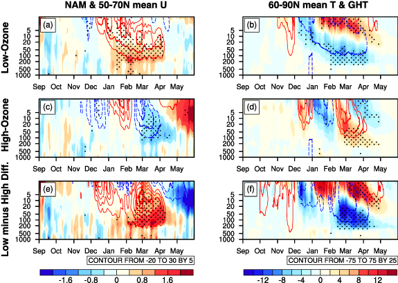
Figure 1. Time-pressure diagrams of composite mean (a), (c), (e) NAM index (shadings) and subpolar (50° N–70° N) average zonal mean zonal wind anomalies (contours, m s−1), and (b), (d), (f) polar cap (60° N–90° N) average anomalies of temperature (shadings, K) and geopotential height (contours, m) respectively for the (a), (b) low Arctic ozone winters and (c), (d) high ozone winters in 1979–2020. Low-minus high-ozone winter differences are displayed in (e), (f). Red (blue) contours denote positive (negative) values. Dotted areas and thickened contours indicate composites above 95% confidence level based on the two-sample t-test.
Download figure:
Standard image High-resolution imageDuring high-ozone winters, the periods of positive and negative NAM and related circulation anomalies at stratospheric levels alternate rapidly (figures 1(c) and (d)). The zonal mean zonal wind anomalies and the stratospheric NAM index (temperature and height anomalies) tend to be negative (positive) during December and March but reverse signs in the periods of January-mid-February and May. Only the anomalies in March, which are simultaneous with the anomalous Arctic ozone, are statistically significant. It looks like a relatively fast-varying stratospheric NAM in the winter and a negative phase of NAM in March often corresponds to the higher Arctic ozone in March.
Differences between low- and high-ozone winters show significant negative (positive) composite mean polar temperature and geipotential height (zonal wind) anomalies associated with positive values of NAM from January to March (figures 1(e) and (f)). This suggests that the polar vortex during the later period of winter played an important role in March ozone depletion, consistent with Calvo et al (2015).
In sum, the composite features of stratospheric polar vortex-related circulation anomalies found in high- and low-ozone winters suggest that not only the intensity and phase of NAM, but also its timescale of variability, are closely linked to Arctic ozone depletion.
3.1.2. Arctic ozone and winter variance of NAMH and NAML
The remarkable interannual variations of the timescales of NAM variability at 100 hPa are clearly manifested by the wavelet spectrum (figure S2) and the winter variance of NAML and NAMH (figure S4). The correlation coefficient between the March Arctic ozone concentration and the normalized winter variance of NAML (NAMH) are negative (positive) but statistically insignificant. This suggests that there seems to be no direct and robust linkage between the winter variance of either NAML or NAMH and the Arctic ozone. One may expect that beside the timescale of NAM variability, the temporal evolution of NAMH and NAML may play a more important role in changing the March Arctic ozone.
3.1.3. Arctic ozone and dominant temporal evolution patterns of NAMH and NAML
We conduct an EOF analysis on the NAM indices at 100 hPa (including NAML and NAMH) considering the day of winter as the spatial dimension and the year of winter as the temporal dimension. The first two spatial modes (i.e. EOF1 and EOF2) capture the dominant temporal evolution patterns of the NAM during winter, the interannual variations of which are measured by the corresponding principal components (i.e. PC1 and PC2).
The temporal evolution pattern represented by the positive phase of the EOF1 mode of NAML (figure 2(a)) is characterized by positive NAML throughout the entire winter (November–March). The positive phase of EOF2 shows the transition from a negative phase of NAM in early winter to a positive phase in late winter since February (figure 2(b)). Seen from figures 3(a) and (b), both of the corresponding PC1 and PC2 are negatively correlated with the Arctic ozone concentration in all winters and below-climatology ozone winters but exhibit no robust relation with Arctic ozone in above-climatology ozone winters. Moreover, the EOF1 of NAML plays a more dominant role in the Arctic ozone depletion according to the more remarkable polarity shift of PC1 than PC2. In particular, during the 17 below-climatology ozone winters, PC1 is positive in 13 winters and close to zero in the remaining 4, while PC2 is positive (negative) in 10 (7) winters. This indicates that a continuously strong stratospheric polar vortex in winter plays a critical role in the Arctic ozone depletion. The above-climatology Arctic ozone, however, might be dominantly modified by synoptic-scale physical processes and other chemical processes besides the low-frequency variations of stratospheric polar vortex.

Figure 2. The temporal patterns of the first leading two EOF modes of (a), (b) NAML and (c), (d) NAMH at 100 hPa in winters from 1979 to 2020.
Download figure:
Standard image High-resolution image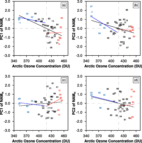
Figure 3. Scatterplots of the (a) PC1 and (b) PC2 of NAML, (c) PC1 and (d) PC2 of NAMH versus the March ozone concentration averaged over the Arctic region with the numbers representing the year. The years with ozone concentration <−1 (>1) SD used for composites in figure 1 are highlighted by blue (red) numbers. Black, blue (red) lines represent the linear fitted line derived from all winters and winters with March Arctic ozone concentration below (above) the climatological mean (418 DU), respectively. The solid (dashed) lines represent the linear fitting statistically significant (insignificant) at 95% confidence level.
Download figure:
Standard image High-resolution imageThe temporal evolution pattern represented by the EOF1 mode of NAMH at 100 hPa (figure 2(c)) is mainly characterized by large positive values from late January to February but negative values in March. We see no significant correlation between the PC1 of NAMH and the Arctic ozone concentration (figure 3(c)), indicating that a relatively fast change of stratospheric NAM in the late winter is not able to result in significant changes of Arctic ozone. The EOF2 mode (figure 2(d)) represents the fast variations of polar vortex mainly in the early winter, characterized by positive values in November followed by negative values in December. The PC2 of NAMH is found to be significantly negatively correlated with Arctic ozone concentration in below-climatology ozone winters (figure 3(d)). This suggests that one or two rounds of fast weakening of stratospheric polar vortex in late November and mid-December are likely to be followed by ozone depletion in March, which can also be seen from figures 1(a) and (b).
We further examine the linkage of March Arctic ozone to negative NAMH events as well as their extreme counterparts (i.e. SSW events) that occurred during the selected periods: 1 November to 17 November, 18 November to 19 December, 21 January to 24 February, 25 February to 31 March. They are selected based on the dominant temporal evolution patterns of NAMH (figures 2(c) and (d)). It is seen from figure 4(a) that in winters with negative NAMH events occurring in the autumn period (1 November to 17 November), the probability density function (PDF) of daily Arctic ozone concentration in March being less than −1 SD is about 9% lower than climatology. Contrastingly, in figure 4(b), for winters with negative NAMH events and major SSW events occurred in the early winter period (18 November to 19 December), the PDF of March Arctic ozone concentration being less than −1 SD increases significantly compared with climatology. Major SSWs correspond to even higher values of PDF toward smaller amounts of ozone. Thus, negative NAMH events and major SSWs during early winter may contribute to the March ozone depletion, supporting the negative relationship between March ozone and PC2 of NAMH in winters with lower ozone (figure 3(d)). Note that the total number of the SSW events in early winter is small and needs further evidence when the data range is extended in future.
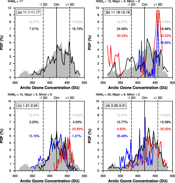
Figure 4. Probability density function (PDF, %) of daily polar-averaged total column ozone concentration in March of all winters (gray shading) and in winters with negative NAMH events (black curve), major/minor SSW events (red/blue curve) occurred in four periods. The four periods are selected because during the 1st and 2nd (3rd and 4th) periods, the EOF2 (EOF1) of NAMH show large positive or negative values (figures 2(c) and (d)). The solid and dash lines respectively indicate the climatological value and ±1 SD of ozone. The total number of years are marked on the top and the probabilities of ozone concentration <−1 SD (>1 SD) are listed at the left (right) column.
Download figure:
Standard image High-resolution imageDifferently, in winters with negative NAMH events and major SSW events occurred in late winter, there is no significant increase in the probability of March ozone being less than −1 SD and opposite shift of PDF can be seen between winters with major and minor SSW events that occurred from 25 February to 31 March (figures 4(c) and (d)), confirming the insignificant relation between March ozone and PC1 of NAMH (figure 3(c)).
Interestingly, the correlation between PC2 of NAMH and PC1 of NAML are high. This could be attributed to the linkage between SSW in early winter and polar vortex variability in the remaining winter months reported by previous studies (Hu et al 2014, 2015). They found that the major SSW events that occur in the early winter tend to be followed by weakened upward wave propagation from the troposphere that can disturb the stratospheric polar vortex in the remaining winter months, thus leading to a stronger polar vortex from late winter to spring and a later final warming.
3.2. Possible climatic influencing factors for the high- and low-frequency NAM variabilities
What kind of climatic factors can effectively modify the Arctic ozone-related variability of stratospheric NAM (i.e. PC1–2 of NAML and PC2 of NAMH) are next investigated in a census style. The correlation maps between SST and SIC anomalies and ozone-related NAM indices (figures S5 and S6) are used to locate the indices of the dominant variation patterns of SST and Arctic sea ice that are potentially influential to the ozone changes. Displayed in figure 5 are the lead-lag correlations of these SST and sea ice indices in the months from September to March with the ozone-related NAM indices.

Figure 5. The correlations between the (a) PC1 and (b) PC2 of NAML, (c) PC2 of NAMH, with monthly indices from November to March, including the Niño3, Niño3.4, Niño4, PDO, NPGO, AMO, and linearly detrended SIE respectively in the regions of B-K Sea and Baffin Bay. Dotted areas represent correlations above 95% confidence level.
Download figure:
Standard image High-resolution image
There seems to exist a concurrent relation between El Niño-Southern Oscillation (ENSO) and NAML, manifested by the positive correlation between the January Niño 4 index with the PC1 of NAML but negative correlation between January Niño 3 and PC2 of NAML. Combined with the correlation maps of SST anomalies (figures S5 a5 and b5) and previous studies (e.g. Calvo and Marsh 2011), we may conclude that a central-type El Niño year might be a favorable condition for the positive phase of EOF1 of NAML, while a La Niña year is favorable for the positive phase of EOF2 of NAML, both contributing to the Arctic ozone depletion. This is related to the relatively normal or colder polar stratosphere during boreal winter under these two conditions. Zubiaurre and Calvo (2012) pointed out that the anomalous warming in the polar stratosphere, which is typical of canonical El Niño episodes as reported by previous studies (e.g. Van Loon and Labitzke 1987, Camp and Tung 2007, Garfinkel and Hartmann 2007, Cagnazzo et al 2009, Lan et al 2012), is not statistically significant during El Niño Modoki events. The cooling in the polar stratosphere and weakened circulation is stronger in response to a La Niña due to the resultant decrease in planetary wave activity in the extratropical stratosphere (García‐Herrera et al 2006, Simpson et al 2011, Oman et al 2013, Neu et al 2014, Rao and Ren 2016a, 2016b).
The PC1 of NAML and PC2 of NAMH are found to be closely related to the NPGO and the AMO. The NPGO index in the winter months shows concurrent negative correlations with both PC1 of NAML and PC2 of NAMH (figures 5(a) and (c)). This suggests that the warm North Pacific SST anomalies with the negative phase of NPGO in the winter are favorable conditions for a strengthened stratospheric polar vortex in the entire winter, preceded by a possible short-lasting weaker polar vortex event in the early winter. This is probably because the warmer North Pacific SSTs always weaken the Aleutian low and the wavenumber-1 wave activity as well as its upward propagation (Li et al 2017, Hu et al 2018, 2019), thus contributing to a stronger stratospheric polar vortex in winter. This result also supports Xia et al (2021), who states that the 2020 Arctic ozone depletion is likely caused by North Pacific warm SST anomalies. Moreover, the PC1 of NAML is negatively correlated with the AMO index not only in the concurrent winter, but also in the preceding September–October (figures 7(a) and S7(a)). This may be due to the fact that the SST anomalies corresponding to the positive phase of AMO in the Autumn can excite a wave train pattern that disturbs the polar vortex and vice versa (Yu and Sun 2020).
In addition to SST forcing, the linearly detrended Arctic sea ice changes show a significant relationship with the NAML (figure S6). The SIE in the B-K Sea in November and SIE in Baffin Bay from February to March are positively correlated with the PC1 of NAML (figure 5(a)). This suggests that higher sea ice often favors a stronger stratospheric polar vortex in winter, confirming findings in previous studies (Li and Wang 2012, Furtado et al 2016, Zhang et al 2020). Seen from figure 5(b), the SIE in Baffin Bay from December to February is negatively correlated with the PC2 of NAML, while the SIE in the B-K Sea from December to March is positively correlated with the PC1 of NAML. This suggests that lower sea ice in Baffin Bay, but more sea ice in the B-K Sea, could mainly favor a subseasonal reversal from a weaker polar vortex in early winter to a stronger polar vortex in the late winter months (February–March). Such reversal could be related to the modulation by sea ice in these two regions over the vertical propagation of planetary waves (Dai and Fan 2022).
To test the usefulness of these climatic forcings in indicating Arctic ozone changes, we looked at the three ozone depletion winters and found that the equatorial Pacific SSTs were warmer in January, the North Pacific SST were consistently warmer from January to February, while the Atlantic SSTs were basically colder from autumn to early winter (particularly for 2019/2020 winter), and the SIE especially in the B-K Sea showed relatively larger values during September to March in 1996/1997 and 2019/2020 winter compared with the neighboring years (not shown).
4. Conclusions
This study investigates the relationship between Arctic ozone concentration in March and the stratospheric NAM variabilities in winter at relatively low frequencies (>4 months) and high frequencies (<2 months). The results reveal that not only the positive phase of NAM and the stronger intensity of stratospheric polar vortex, but also their persistence play important roles in the Arctic ozone depletion. The relationship between Arctic ozone and the low-frequency component of lower-stratospheric NAM (NAML) are much closer than that between Arctic ozone and the high-frequency component (NAMH). Key results include:
- (i)During low-ozone winters, positive NAM signals propagated downward and stalled in the lower stratosphere from mid-December to March, while during high-ozone winters, the stratospheric NAM changed its phase frequently. The largest difference in the persistence of the NAM phase between low- and high-ozone winters lies around 100 hPa. Therefore, more active wave dynamical processes that are dominated by shorter timescales are involved in high-ozone winters, while the stratospheric polar vortex is less disturbed and might be affected by longer timescales of chemical-radiative processes in low-ozone winters.
- (ii)The temporal evolution of 100 hPa NAML plays a more important role in changing the Arctic ozone. A persistently strong stratospheric polar vortex in winter (especially February–March) plays a more critical role than a short-lasting extremely strong vortex in contributing to the Arctic ozone depletion. Negative NAMH events or major SSW events in early winter might be a precursor for Arctic ozone depletion in March.
- (iii)The ozone-related NAM changes are further related to the warm SST anomalies in the North Pacific in December and January, the 'central-type' El Niño-like or La Niña-like equatorial SST anomalies in January and the negative phase of AMO and higher sea ice in the B-K Sea from late-autumn to early-spring.
Acknowledgments
The research was jointly supported by the National Natural Science Foundation of China (42375060, 42088101, 42075062), Project of Shenzhen Science and Technology Innovation Commission (KCXFZ20201221173610028), the Natural Science Foundation of Jiangsu Province (BK20211288). The MSR-2 ozone data can be found at: www.temis.nl/protocols/O3global.php. SIC and SIE: https://psl.noaa.gov/data/gridded/data.noaa.oisst.v2.html and https://nsidc.org/data/g02135/versions/3. PDO, NPGO and AMO indices: http://research.jisao.washington.edu/data_sets/pdo/, www.o3d.org/npgo/ and https://psl.noaa.gov/data/correlation/amon.us.data.
Data availability statement
The authors declare that data sets for this research are available in the following online repository: https://cds.climate.copernicus.eu/.
The data that support the findings of this study are openly available at the following URL/DOI: https://cds.climate.copernicus.eu/cdsapp#!/dataset/reanalysis-era5-pressure-levels.
Supplementary data (5.2 MB DOCX)