On the approximations to fractional nonlinear damped Burger’s-type equations that arise in fluids and plasmas using Aboodh residual power series and Aboodh transform iteration methods

Noor, Saima; Albalawi, Wedad; Shah, Rasool; Al-Sawalha, M. Mossa; Ismaeel, Sherif M. E.; El-Tantawy, S. A.

doi:10.3389/fphy.2024.1374481

ORIGINAL RESEARCH article

Front. Phys., 02 April 2024
Sec. Mathematical Physics
Volume 12 - 2024 | https://doi.org/10.3389/fphy.2024.1374481

On the approximations to fractional nonlinear damped Burger’s-type equations that arise in fluids and plasmas using Aboodh residual power series and Aboodh transform iteration methods

Saima Noor^1,2* www.frontiersin.org

Wedad Albalawi³

Rasool Shah⁴* www.frontiersin.org

M. Mossa Al-Sawalha⁵ www.frontiersin.org

Sherif M. E. Ismaeel^6,7

S. A. El-Tantawy^8,9

¹Department of Basic Sciences, General Administration of Preparatory Year, King Faisal University, Al Ahsa, Saudi Arabia
²Department of Mathematics and Statistics, College of Science, King Faisal University, Al Ahsa, Saudi Arabia
³Department of Mathematical Sciences, College of Science, Princess Nourah bint Abdulrahman University, Riyadh, Saudi Arabia
⁴Department of Computer Science and Mathematics, Lebanese American University, Beirut, Lebanon
⁵Department of Mathematics, College of Science, University of Ha’il, Ha’il, Saudi Arabia
⁶Department of Physics, College of Science and Humanities in Al-Kharj, Prince Sattam Bin Abdulaziz University, Al-Kharj, Saudi Arabia
⁷Department of Physics, Faculty of Science, Ain Shams University, Cairo, Egypt
⁸Department of Physics, Faculty of Science, Port Said University, Port Said, Egypt
⁹Research Center for Physics (RCP), Department of Physics, Faculty of Science and Arts, Al-Mikhwah, Al-Baha University, Al-Baha, Saudi Arabia

Damped Burger’s equation describes the characteristics of one-dimensional nonlinear shock waves in the presence of damping effects and is significant in fluid dynamics, plasma physics, and other fields. Due to the potential applications of this equation, thus the objective of this investigation is to solve and analyze the time fractional form of this equation using methods with precise efficiency, high accuracy, ease of application and calculation, and flexibility in dealing with more complicated equations, which are called the Aboodh residual power series method and the Aboodh transform iteration method (ATIM) within the Caputo operator framework. Also, this study intends to further our understanding of the dynamic characteristics of solutions to the Damped Burger’s equation and to assess the effectiveness of the proposed methods in addressing nonlinear fractional partial differential equations. The two proposed methods are highly effective mathematical techniques for studying more complicated nonlinear differential equations. They can produce precise approximate solutions for intricate evolution equations beyond the specific examined equation. In addition to the proposed methods, the fractional derivatives are processed using the Caputo operator. The Caputo operator enhances the representation of fractional derivatives by providing a more accurate portrayal of the underlying physical processes. Based on the proposed two approaches, a set of approximations to damped Burger’s equation are derived. These approximations are discussed graphically and numerically by presenting a set of two- and three-dimensional graphs. In addition, these approximations are analyzed numerically in several tables, including the absolute error for each approximate solution compared to the exact solution for the integer case. Furthermore, the effect of the fractional parameter on the behavior of the derived approximations is examined and discussed.

1 Introduction

There has been a growing interest in fractional differential equations (FDEs) in recent years. The fractional approach is a strong modeling paradigm in mechanics and materials, wave propagation, anomalous diffusion, and turbulence. Natural phenomena exhibit anomalous diffusion, in which the underlying stochastic process does not follow Brownian motion. Compared to the Gaussian process, the mean-square variance may rise more quickly for superdiffusion or more slowly for subdiffusion. Due to long-range correlations in dynamics or anomalously large particle jumps, non-Gaussion diffusion models can be constructed utilizing nonlocal-in-time or nonlocal in-space operators, such as Caputo or Riemann–Liouville derivatives. The advantage of the fractional model is that anomalous diffusion is well described [1–11]. The singularity of the kernel poses a difficulty for the authors of Caputo and Riemann derivatives. Considering the fact that the kernel is utilized to clarify the memory impact of the physical system, it is indisputable that this limitation restricts both derivatives from accurately assessing the full effect of the memory. Caputo and Fabrizio (CF) [12] introduced a novel fractional operator with an exponential kernel during the mid-1990s as part of their effort to do so. The utilization of the nonsingular kernel of this derivative produces more logical outcomes when compared to the conventional method. A compilation of CF operator implementations has been expanded around in Ref. [13–15]. The research articles cited encompass a diverse range of topics within the field of control systems, vibration isolation, and neural network approximation. Guo et al. delve into fixed-time safe tracking control and non-singular fixed-time tracking control of uncertain nonlinear systems [16, 17] 3. Lu et al. focus on nonlinear vibration isolation systems with high-static-low-dynamic stiffness [18, 19]. Additionally, Luo et al. explore adaptive optimal control of affine nonlinear systems using identifier-critic neural network approximation [20]. These studies contribute valuable insights and advancements to their respective areas, showcasing the ongoing innovation and research efforts in control theory and engineering applications.

Determining an exact solution to partial differential equations (PDEs) of fractional order is exceedingly challenging. The ability to precisely and numerically solve such equations is critical in applied mathematics. As a result, innovative approaches have been developed to obtain analytical solutions that demonstrate a significant level of accuracy compared to the precise solutions [21–23]. The resolution of differential equations often involves the utilization of integral transformations. Employing integral transformations makes resolving IVPs and BVPs in differential and integral equations possible efficiently. An extensive array of scholars examined the consequences of various integral transforms applied to distinct classes of differential equations [24–26]. The Laplace transform is the integral transform that is most commonly utilized [27]. In 1998, Watugala [28] introduced the Sumudu transform, which proved to be an efficient approach to addressing control engineering and differential equations challenges. In 2011, T. Elzaki and S. Elzaki proposed the “Elzaki Transform” as an innovative integral transform; its utilization in the resolution of partial differential equations has since become widespread [29]. In 2013, Aboodh additionally presented the “Aboodh Transform (AT)” and applied it to the resolution of PDEs [30]. A variety of transformations are documented in the literature.

Omar Abu Arqub created the RPSM in 2013 [31]. The RPSM combines the residual error function with Taylor’s series. After that, this approach was used to find convergence series approximations for both nonlinear and linear differential equations. The RPSM was first introduced in 2013 to solve fuzzy differential equations. More improvements were made to this technique. For instance, Arqub et al. [32] developed a novel collection of RPSM algorithms to promptly find power series solutions for ordinary DEs. Furthermore, Arqub et al. [33] introduced a novel and appealing RPSM method for fractional-order nonlinear boundary value problems. El-Ajou et al. [34] introduced an innovative iterative approach utilizing RPSM to approximate fractional-order solutions to the KdV-burgers equations. A novel approach was introduced by Xu et al. [35], which involved fractional power series solutions for Boussinesq DEs of the second and fourth orders. Zhang et al. [36] synthesized least square methods and RPSM to develop a robust numerical technique. Consult [37–39] for additional readings on RPSM in greater depth.

Scientists utilized two distinct methodologies to solve fractional-order differential equations (FODEs). A sequence of solutions to the new equation form is obtained by mapping the original equation onto the space produced by the AT [40]. The solution to the original equation is obtained by applying the inverse Aboodh transform. Components of the Sumudu transform, and the homotopy perturbation approach are combined in this novel method. As power series expansions, the novel technique, which does not require discretization, linearization, or perturbation, can solve both linear and nonlinear PDEs. The determination of the coefficients can be accomplished through a limited number of calculations, in contrast to RPSM, which necessitates numerous iterations of fractional derivative computations during the solution phases. The proposed methodology has the potential to yield an accurate and closed-form approximation by leveraging a rapid convergence series.

For solving fractional differential equations, the Aboodh transform iteration method (ATIM) [41–43] and the Aboodh residual power series method (ARPSM) [44, 45] are regarded as the most straightforward techniques. These methods generate numerical approximations for solutions to linear and nonlinear differential equations without requiring discretization or linearization and immediately and visibly display the symbolic terms of analytical solutions. Comparing and contrasting the effectiveness of ARPSM and ATIM in solving nonlinear PDEs, specifically damped Burger’s equation, is the primary objective of this study. It is worth mentioning that these two methods have been employed to resolve many fractional differential problems, both linear and nonlinear.

2 Fundamental concepts

Definition 2.1. [46] It is assumed that the function Θ(ζ, η) is of exponential order and piecewise continuous.

For τ ≥ 0, the AT of Θ(ζ, η) is defined as follows:

A [Θ (ζ, η)] = Λ (ζ, ϵ) = \frac{1}{ϵ} \int_{0}^{\infty} Θ (ζ, η) e^{- η ϵ} d η, r_{1} \leq ϵ \leq r_{2} .

Below is a description of the inverse of AT:

A^{- 1} [Λ (ζ, ϵ)] = Θ (ζ, η) = \frac{1}{2 π i} \int_{u - i \infty}^{u + i \infty} Λ (ζ, η) ϵ e^{η ϵ} d η

Where $ζ = (ζ_{1}, ζ_{2}, \dots, ζ_{p}) \in R$ and $p \in N$ .

Lemma 2.1. [47, 48] Two functions of exponential order, Θ₁(ζ, η) and Θ₂(ζ, η), are defined. They are piecewise continuous on $[0, \infty$ ]. Let us assume that A[Θ₁(ζ, η)] = Λ₁(ζ, η), A[Θ₂(ζ, η)] = Λ₂(ζ, η) and λ₁, λ₂ are real constants. Thus, the following features are valid:

1. A [λ₁Θ₁ (ζ, η) + λ₂Θ₂ (ζ, η)] = λ₁Λ₁ (ζ, ϵ) + λ₂Λ₂ (ζ, η),

2. A⁻¹ [λ₁Λ₁ (ζ, η) + λ₂Λ₂ (ζ, η)] = λ₁Θ₁ (ζ, ϵ) + λ₂Θ₂ (ζ, η),

3. $A [J_{η}^{p} Θ (ζ, η)] = \frac{Λ (ζ, ϵ)}{ϵ^{p}}$ ,

4. $A [D_{η}^{p} Θ (ζ, η)] = ϵ^{p} Λ (ζ, ϵ) - \sum_{K = 0}^{r - 1} \frac{Θ^{K} (ζ, 0)}{ϵ^{K - p + 2}}, r - 1 < p \leq r, r \in N$ .

Definition 2.2. [49] The Caputo defines the fractional derivative of the function Θ(ζ, η) in terms of order p.

D_{η}^{p} Θ (ζ, η) = J_{η}^{m - p} Θ^{(m)} (ζ, η), r \geq 0, m - 1 < p \leq m,

where $ζ = (ζ_{1}, ζ_{2}, \dots, ζ_{p}) \in R^{p}$ and $m, p \in R, J_{η}^{m - p}$ is the R-L integral of Θ(ζ, η).

Definition 2.3. [50] The power series has the following form.

\sum_{r = 0}^{\infty} ℏ_{r} (ζ) {(η - η_{0})}^{r p} = ℏ_{0} {(η - η_{0})}^{0} + ℏ_{1} {(η - η_{0})}^{p} + ℏ_{2} {(η - η_{0})}^{2 p} + \dots,

where $ζ = (ζ_{1}, ζ_{2}, \dots, ζ_{p}) \in R^{p}$ and $p \in N$ . This kind of series is called a multiple fractional power series (MFPS) for η₀, where the variable is η and the series coefficients are ℏ_r(ζ)′s.

Lemma 2.2. Let us assume that Θ(ζ, η) is the exponential order function. In this case, A[Θ(ζ, η)] = Λ(ζ, ϵ) is the definition of the AT. Therefore,

A [D_{η}^{r p} Θ (ζ, η)] = ϵ^{r p} Λ (ζ, ϵ) - \sum_{j = 0}^{r - 1} ϵ^{p (r - j) - 2} D_{η}^{j p} Θ (ζ, 0), 0 < p \leq 1, (1)

where $ζ = (ζ_{1}, ζ_{2}, \dots, ζ_{p}) \in R^{p}$ and $p \in N$ and $D_{η}^{r p} = D_{η}^{p} . D_{η}^{p} . \dots . D_{η}^{p} (r - t i m e s)$

Proof. We can demonstrate Eq. 2 via induction. The following outcomes arise from selecting r = 1 in Eq. 2:

A [D_{η}^{2 p} Θ (ζ, η)] = ϵ^{2 p} Λ (ζ, ϵ) - ϵ^{2 p - 2} Θ (ζ, 0) - ϵ^{p - 2} D_{η}^{p} Θ (ζ, 0)

For r = 1, Lemma 2.1, part (4), asserts that Eq. 2 is valid. By changing r = 2 in Eq. 2, we get

A [D_{r}^{2 p} Θ (ζ, η)] = ϵ^{2 p} Λ (ζ, ϵ) - ϵ^{2 p - 2} Θ (ζ, 0) - ϵ^{p - 2} D_{η}^{p} Θ (ζ, 0) . (2)

In light of Eq. 2’s left-hand side, we can conclude

L . H . S = A [D_{η}^{2 p} Θ (ζ, η)] . (3)

Eq. 3 may be expressed in the following way:

L . H . S = A [D_{η}^{p} Θ (ζ, η)] . (4)

Let us assume

z (ζ, η) = D_{η}^{p} Θ (ζ, η) . (5)

Thus, Eq. 4 becomes as

L . H . S = A [D_{η}^{p} z (ζ, η)] . (6)

The use of the Caputo type fractional derivative results in a modification of Eq. 6.

L . H . S = A [J^{1 - p} z^{'} (ζ, η)] . (7)

The R-L integral for the AT is found in Eq. 7, which makes it possible to derive the following:

L . H . S = \frac{A [z^{'} (ζ, η)]}{ϵ^{1 - p}} . (8)

Equation 8 is transformed into the following form by using the differential characteristic of the AT:

L . H . S = ϵ^{p} Z (ζ, ϵ) - \frac{z (ζ, 0)}{ϵ^{2 - p}}, (9)

From Eq. 5, we obtain:

Z (ζ, ϵ) = ϵ^{p} Λ (ζ, ϵ) - \frac{Θ (ζ, 0)}{ϵ^{2 - p}},

where A [z (ζ, η)] = Z (ζ, ϵ). Therefore, Eq. 9 is converted to

L . H . S = ϵ^{2 p} Λ (ζ, ϵ) - \frac{Θ (ζ, 0)}{ϵ^{2 - 2 p}} - \frac{D_{η}^{p} Θ (ζ, 0)}{ϵ^{2 - p}}, (10)

According to Eq. 2, then Eq. 10 is compatible. Let us assume the validity of Eq. 2 for r = K. This allows us to change r = K in Eq. 2:

A [D_{η}^{K p} Θ (ζ, η)] = ϵ^{K p} Λ (ζ, ϵ) - \sum_{j = 0}^{K - 1} ϵ^{p (K - j) - 2} D_{η}^{j p} D_{η}^{j p} Θ (ζ, 0), 0 < p \leq 1 . (11)

Proving Eq. 2 for the value of r = K + 1 is the next step. Based on Eq. 2, we may write

A [D_{η}^{(K + 1) p} Θ (ζ, η)] = ϵ^{(K + 1) p} Λ (ζ, ϵ) - \sum_{j = 0}^{K} ϵ^{p ((K + 1) - j) - 2} D_{η}^{j p} Θ (ζ, 0) . (12)

After analysis of the LHS of Eq. 12, we get

L . H . S = A [D_{η}^{K p} (D_{η}^{K p})] . (13)

Suppose that

D_{η}^{K p} = g (ζ, η) .

Equation 13 yields

L . H . S = A [D_{η}^{p} g (ζ, η)] . (14)

By using the R-L integral formula and the Caputo fractional derivative, we may convert Eq. 14 into the following expression.

L . H . S = ϵ^{p} A [D_{η}^{K p} Θ (ζ, η)] - \frac{g (ζ, 0)}{ϵ^{2 - p}} . (15)

Equation 11 is unitized to provide Eq. 15.

L . H . S = ϵ^{r p} Λ (ζ, ϵ) - \sum_{j = 0}^{r - 1} ϵ^{p (r - j) - 2} D_{η}^{j p} Θ (ζ, 0), (16)

Moreover, Eq. 16 yields the following result.

L . H . S = A [D_{η}^{r p} Θ (ζ, 0)] .

Therefore, Eq. 2 holds for r = K + 1. Thus, we used the mathematical induction approach and shows that Eq. 2 holds true for all positive integers.

Extending the concept of multiple fractional A lemma demonstrating Taylor’s formula is shown below. The ARPSM, which will be covered in more detail later on, will benefit from this formula.

Lemma 2.3. Assume that the function Θ(ζ, η) behaves exponentially order. The statement A[Θ(ζ, η)] = Λ(ζ, ϵ) represents the AT of Θ(ζ, η), and it is multiple fractional Taylor’s series expressed as:

Λ (ζ, ϵ) = \sum_{r = 0}^{\infty} \frac{ℏ_{r} (ζ)}{ϵ^{r p + 2}}, ϵ > 0, (17)

where, $ζ = (s_{1}, ζ_{2}, \dots, ζ_{p}) \in R^{p}, p \in N$ .

Proof. Now we examine the fractional order of Taylor’s series as

Θ (ζ, η) = ℏ_{0} (ζ) + ℏ_{1} (ζ) \frac{η^{p}}{Γ [p + 1]} + + ℏ_{2} (ζ) \frac{η^{2 p}}{Γ [2 p + 1]} + \dots . (18)

Equation 18 may be transformed using the AT to get the following equality:

A [Θ (ζ, η)] = A [ℏ_{0} (ζ)] + A [ℏ_{1} (ζ) \frac{η^{p}}{Γ [p + 1]}] + A [ℏ_{1} (ζ) \frac{η^{2 p}}{Γ [2 p + 1]}] + \dots

For this, we use the AT’s characteristics.

A [Θ (ζ, η)] = ℏ_{0} (ζ) \frac{1}{ϵ^{2}} + ℏ_{1} (ζ) \frac{Γ [p + 1]}{Γ [p + 1]} \frac{1}{ϵ^{p + 2}} + ℏ_{2} (ζ) \frac{Γ [2 p + 1]}{Γ [2 p + 1]} \frac{1}{ϵ^{2 p + 2}} \dots

Hence, in the AT, we obtains (17), a new version of Taylor’s series.

Lemma 2.4. Define the MFPS representation of the function expressed in the new form of Taylor’s series (17) as A[Θ(ζ, η)] = Λ(ζ, ϵ). Next, we have

ℏ_{0} (ζ) = \lim_{ϵ \to \infty} ϵ^{2} Λ (ζ, ϵ) = Θ (ζ, 0) . (19)

Proof. The subsequent is derived from the new form of Taylor’s series:

ℏ_{0} (ζ) = ϵ^{2} Λ (ζ, ϵ) - \frac{ℏ_{1} (ζ)}{ϵ^{p}} - \frac{ℏ_{2} (ζ)}{ϵ^{2 p}} - \dots (20)

The required result, denoted by Eq. 20, is obtained by applying lim_ϵ→∞ to Eq. 19 and performing a brief computation.

Theorem 2.5. Let us suppose that the function A[Θ(ζ, η)] = Λ(ζ, ϵ) has MFPS form given by

Λ (ζ, ϵ) = \sum_{0}^{\infty} \frac{ℏ_{r} (ζ)}{ϵ^{r p + 2}}, ϵ > 0,

where $ζ = (ζ_{1}, ζ_{2}, \dots, ζ_{p}) \in R^{p}$ and $p \in N$ . Then we have

ℏ_{r} (ζ) = D_{r}^{r p} Θ (ζ, 0),

where, $D_{η}^{r p} = D_{η}^{p} . D_{η}^{p} . \dots . D_{η}^{p} (r - t i m e s)$ .

Proof. This is the revised version of the Taylor’s series that we have.

ℏ_{1} (ζ) = ϵ^{p + 2} Λ (ζ, ϵ) - ϵ^{p} ℏ_{0} (ζ) - \frac{ℏ_{2} (ζ)}{ϵ^{p}} - \frac{ℏ_{3} (ζ)}{ϵ^{2 p}} - \dots (21)

Using Eq. 21 and the lim_ϵ→∞, we are able to get

ℏ_{1} (ζ) = \lim_{ϵ \to \infty} (ϵ^{p + 2} Λ (ζ, ϵ) - ϵ^{p} ℏ_{0} (ζ)) - \lim_{ϵ \to \infty} \frac{ℏ_{2} (ζ)}{ϵ^{p}} - \lim_{ϵ \to \infty} \frac{ℏ_{3} (ζ)}{ϵ^{2 p}} - \dots

Taking limit, we arrive at the equality that follows:

ℏ_{1} (ζ) = \lim_{ϵ \to \infty} (ϵ^{p + 2} Λ (ζ, ϵ) - ϵ^{p} ℏ_{0} (ζ)) . (22)

Following is the result that is obtained by applying Lemma (2.2) to Eq. 22:

ℏ_{1} (ζ) = \lim_{ϵ \to \infty} (ϵ^{2} A [D_{η}^{p} Θ (ζ, η)] (ϵ)) . (23)

Through the use of Lemma (2.3) to Eq. 23, the equation is changed into

ℏ_{1} (ζ) = D_{η}^{p} Θ (ζ, 0) .

Once again, by taking into consideration the new implementation of Taylor’s series and assuming limit ϵ → ∞, we have arrived at the result that

ℏ_{2} (ζ) = ϵ^{2 p + 2} Λ (ζ, ϵ) - ϵ^{2 p} ℏ_{0} (ζ) - ϵ^{p} ℏ_{1} (ζ) - \frac{ℏ_{3} (ζ)}{ϵ^{p}} - \dots

Lemma (2.3) leads us to get the following:

ℏ_{2} (ζ) = \lim_{ϵ \to \infty} ϵ^{2} (ϵ^{2 p} Λ (ζ, ϵ) - ϵ^{2 p - 2} ℏ_{0} (ζ) - ϵ^{p - 2} ℏ_{1} (ζ)) . (24)

With the help of Lemmas (2.2) and (2.4), Eq. 24 is transformed into

ℏ_{2} (ζ) = D_{η}^{2 p} Θ (ζ, 0) .

When we apply the same method to the subsequent Taylor’s series, we obtain the following results:

ℏ_{3} (ζ) = \lim_{ϵ \to \infty} ϵ^{2} (A [D_{η}^{2 p} Θ (ζ, p)] (ϵ)) .

The final equation can be found by applying Lemma (2.4).

ℏ_{3} (ζ) = D_{η}^{3 p} Θ (ζ, 0) .

So, in general

ℏ_{r} (ζ) = D_{η}^{r p} Θ (ζ, 0) .

Thus, the proof comes to an end.

In the succeeding theorem, the conditions that determine the convergence of the new version of Taylor’s formula are established and detailed in further depth.

Theorem 2.6. The revised formula for multiple fractional Taylor’s, given in Lemma (2.3), is denoted by the expression A[Θ(ζ, η)] = Λ(ζ, ϵ). The new version of multiple fractional Taylor’s formula’s residual R_K(ζ, ϵ) satisfies the following inequality if $| ϵ^{a} A [D_{η}^{(K + 1) p} Θ (ζ, η)] | \leq T$ , on 0 < ϵ ≤ s is associated with 0 < p ≤ 1:

| R_{K} (ζ, ϵ) | \leq \frac{T}{ϵ^{(K = 1) p + 2}}, 0 < ϵ \leq s .

Proof. To start the proof, Let assume: For r = 0, 1, 2, … , K + 1, $A [D_{η}^{r p} Θ (ζ, η)] (ϵ)$ is defined on 0 < ϵ ≤ s. Let, $| ϵ^{2} A [D_{η^{K + 1}} Θ (ζ, t a u)] | \leq T, o n 0 < ϵ \leq s$ . Based on the revised version of Taylor’s series, determine the following relationship:

R_{K} (ζ, ϵ) = Λ (ζ, ϵ) - \sum_{r = 0}^{K} \frac{ℏ_{r} (ζ)}{ϵ^{r p + 2}} . (25)

Applying Theorem (2.5) allows for the transformation of Eq. 25.

R_{K} (ζ, ϵ) = Λ (ζ, ϵ) - \sum_{r = 0}^{K} \frac{D_{η}^{r p} Θ (ζ, 0)}{ϵ^{r p + 2}} . (26)

It is necessary to multiply ϵ^(K+1)a+2 on both sides of Eq. 26 which leads to

ϵ^{(K + 1) p + 2} R_{K} (ζ, ϵ) = ϵ^{2} (ϵ^{(K + 1) p} Λ (ζ, ϵ) - \sum_{r = 0}^{K} ϵ^{(K + 1 - r) p - 2} D_{η}^{r p} Θ (ζ, 0)) . (27)

The use of Lemma (2.2) to Eq. 27 results in

ϵ^{(K + 1) p + 2} R_{K} (ζ, ϵ) = ϵ^{2} A [D_{η}^{(K + 1) p} Θ (ζ, η)] . (28)

Equation 28 is obtained by applying the absolute sign to the equation.

| ϵ^{(K + 1) p + 2} R_{K} (ζ, ϵ) | = | ϵ^{2} A [D_{η}^{(K + 1) p} Θ (ζ, η)] | . (29)

By applied the condition given in Eq. 29, we can arrive at the result as will be given below.

\frac{- T}{ϵ^{(K + 1) p + 2}} \leq R_{K} (ζ, ϵ) \leq \frac{T}{ϵ^{(K + 1) p + 2}} . (30)

Equation 30 yields the required result.

| R_{K} (ζ, ϵ) | \leq \frac{T}{ϵ^{(K + 1) p + 2}} .

Hence, a novel criterion for series convergence is established.

3 A route map describing the methods

3.1 Solving time-fractional PDEs with variable coefficients by use of the ARPSM process

We detail the ARPSM rules that was used to resolve our underlying model.

Step 1:. Finding the general equation’s simplified form yields

D_{η}^{q p} Θ (ζ, η) + ϑ (ζ) N (Θ) - ζ (ζ, Θ) = 0, (31)

Step 2:. The AT is applied on both sides of Eq. 31 in order to get

A [D_{η}^{q p} Θ (ζ, η) + ϑ (ζ) N (Θ) - ζ (ζ, Θ)] = 0, (32)

The use of Lemma (2.2) transforms Eq. 32 into.

Λ (ζ, s) = \sum_{j = 0}^{q - 1} \frac{D_{η}^{j} Θ (ζ, 0)}{s^{q p + 2}} - \frac{ϑ (ζ) Y (s)}{s^{q p}} + \frac{F (ζ, s)}{s^{q p}}, (33)

where, A [ζ(ζ, Θ)] = F (ζ, s), A [N(Θ)] = Y(s).

Step 3:. You should take into consideration the form that the solution to Eq. 33 takes:

Λ (ζ, s) = \sum_{r = 0}^{\infty} \frac{ℏ_{r} (ζ)}{s^{r p + 2}}, s > 0,

Step 4:. In order to proceed further, you will need to follow these steps:

ℏ_{0} (ζ) = \lim_{s \to \infty} s^{2} Λ (ζ, s) = Θ (ζ, 0),

Through the use of Theorem 2.6, the following results are derived.

ℏ_{1} (ζ) = D_{η}^{p} Θ (ζ, 0),

ℏ_{2} (ζ) = D_{η}^{2 p} Θ (ζ, 0),

⋮

ℏ_{w} (ζ) = D_{η}^{w p} Θ (ζ, 0),

Step 5:. After Kth truncation, get the Λ(ζ, s) series in the following way:

Λ_{K} (ζ, s) = \sum_{r = 0}^{K} \frac{ℏ_{r} (ζ)}{s^{r p + 2}}, s > 0,

Λ_{K} (ζ, s) = \frac{ℏ_{0} (ζ)}{s^{2}} + \frac{ℏ_{1} (ζ)}{s^{p + 2}} + \dots + \frac{ℏ_{w} (ζ)}{s^{w p + 2}} + \sum_{r = w + 1}^{K} \frac{ℏ_{r} (ζ)}{s^{r p + 2}},

Step 6:. Consider both the Aboodh residual function (ARF) from equation Eq. 33 and the K^th-truncated ARF separately to get

A R e s (ζ, s) = Λ (ζ, s) - \sum_{j = 0}^{q - 1} \frac{D_{η}^{j} Θ (ζ, 0)}{s^{j p + 2}} + \frac{ϑ (ζ) Y (s)}{s^{j p}} - \frac{F (ζ, s)}{s^{j p}},

and

A R e s_{K} (ζ, s) = Λ_{K} (ζ, s) - \sum_{j = 0}^{q - 1} \frac{D_{η}^{j} Θ (ζ, 0)}{s^{j p + 2}} + \frac{ϑ (ζ) Y (s)}{s^{j p}} - \frac{F (ζ, s)}{s^{j p}} . (34)

Step 7:. Instead of its expansion form, put Λ_K(ζ, s) into Eq. 34.

\begin{aligned} A R e s_{K} (ζ, s) = (\frac{ℏ_{0} (ζ)}{s^{2}} + \frac{ℏ_{1} (ζ)}{s^{p + 2}} + \dots + \frac{ℏ_{w} (ζ)}{s^{w p + 2}} + \sum_{r = w + 1}^{K} \frac{ℏ_{r} (ζ)}{s^{r p + 2}}) \\ - \sum_{j = 0}^{q - 1} \frac{D_{η}^{j} Θ (ζ, 0)}{s^{j p + 2}} + \frac{ϑ (ζ) Y (s)}{s^{j p}} - \frac{F (ζ, s)}{s^{j p}} . \end{aligned} (35)

Step 8:. To solve Eq. 35, multiply both sides of the equation by s^Kp+2.

\begin{aligned} s^{K p + 2} A R e s_{K} (ζ, s) = s^{K p + 2} (\frac{ℏ_{0} (ζ)}{s^{2}} + \frac{ℏ_{1} (ζ)}{s^{p + 2}} + \dots + \frac{ℏ_{w} (ζ)}{s^{w p + 2}} + \sum_{r = w + 1}^{K} \frac{ℏ_{r} (ζ)}{s^{r p + 2}} \\ - \sum_{j = 0}^{q - 1} \frac{D_{η}^{j} Θ (ζ, 0)}{s^{j p + 2}} + \frac{ϑ (ζ) Y (s)}{s^{j p}} - \frac{F (ζ, s)}{s^{j p}}) . \end{aligned} (36)

Step 9:. With respect to lim_s→∞, evaluating both sides of Eq. 36.

\begin{aligned} \lim_{s \to \infty} s^{K p + 2} A R e s_{K} (ζ, s) = \lim_{s \to \infty} s^{K p + 2} (\frac{ℏ_{0} (ζ)}{s^{2}} + \frac{ℏ_{1} (ζ)}{s^{p + 2}} + \dots + \frac{ℏ_{w} (ζ)}{s^{w p + 2}} + \sum_{r = w + 1}^{K} \frac{ℏ_{r} (ζ)}{s^{r p + 2}} \\ - \sum_{j = 0}^{q - 1} \frac{D_{η}^{j} Θ (ζ, 0)}{s^{j p + 2}} + \frac{ϑ (ζ) Y (s)}{s^{j p}} - \frac{F (ζ, s)}{s^{j p}}) . \end{aligned}

Step 10:. By solving the provided equation, determine the value of ℏ_K(ζ).

\lim_{s \to \infty} (s^{K p + 2} A R e s_{K} (ζ, s)) = 0,

where K = w + 1, w + 2, ⋯.

Step 11:. Replace the values of ℏ_K(ζ) with a K-truncated series of Λ(ζ, s) to get the K-approximate solution of Eq. 33.

Step 12:. The K-approximate solution Θ_K(ζ, η) may be obtained by solving Λ_K(ζ, s) with the inverse of AT.

3.2 Problem 1

Let us consider the following time fractional PDE [51]:

\begin{aligned} D_{η}^{p} Θ (ζ, η) + Θ (ζ, η) \frac{\partial^{3} Θ (ζ, η)}{\partial ζ^{3}} - \frac{\partial Θ (ζ, η)}{\partial ζ} \frac{\partial^{2} Θ (ζ, η)}{\partial ζ^{2}} - \frac{\partial^{2} Θ (ζ, η)}{\partial ζ^{2}} = 0, where 0 < p \leq 1 \end{aligned} (37)

with the following IC’s:

\begin{aligned} Θ (ζ, 0) = \frac{e^{ζ / 4}}{4} . \end{aligned} (38)

and the following exact solution

\begin{aligned} Θ (ζ, η) = \frac{1}{4} e^{\frac{1}{4} (\frac{η}{4} + ζ)} . \end{aligned} (39)

Equation 38 is used, and AT is applied to Eq. 37 to get

\begin{aligned} Θ (ζ, s) - \frac{\frac{e^{ζ / 4}}{4}}{s^{2}} + \frac{1}{s^{p}} A_{η} [A_{η}^{- 1} Θ (ζ, s) \times \frac{\partial^{3} A_{η}^{- 1} Θ (ζ, s)}{\partial ζ^{3}}] - \frac{1}{s^{p}} A_{η} [\frac{\partial A_{η}^{- 1} Θ (ζ, s)}{\partial ζ} \frac{\partial^{2} A_{η}^{- 1} Θ (ζ, s)}{\partial ζ^{2}}] \\ - \frac{1}{s^{p}} [\frac{\partial^{2} Θ (ζ, s)}{\partial ζ^{2}}] = 0, \end{aligned} (40)

Thus, the kth-truncated term series are

\begin{aligned} Θ (ζ s) = \frac{\frac{e^{ζ / 4}}{4}}{s^{2}} + \sum_{r = 1}^{k} \frac{f_{r} (ζ, s)}{s^{r p + 1}}, r = 1,2,3,4 \dots \end{aligned} (41)

The ARFs read

\begin{aligned} A_{η} R e s (ζ, s) = Θ (ζ, s) - \frac{\frac{e^{ζ / 4}}{4}}{s^{2}} + \frac{1}{s^{p}} A_{η} [A_{η}^{- 1} Θ (ζ, s) \times \frac{\partial^{3} A_{η}^{- 1} Θ (ζ, s)}{\partial ζ^{3}}] - \frac{1}{s^{p}} A_{η} [\frac{\partial A_{η}^{- 1} Θ (ζ, s)}{\partial ζ} \frac{\partial^{2} A_{η}^{- 1} Θ (ζ, s)}{\partial ζ^{2}}] \\ - \frac{1}{s^{p}} [\frac{\partial^{2} Θ (ζ, s)}{\partial ζ^{2}}] = 0, \end{aligned} (42)

and the kth-LRFs as:

\begin{aligned} A_{η} R e s_{k} (ζ, s) = Θ_{k} (ζ, s) - \frac{\frac{e^{ζ / 4}}{4}}{s^{2}} + \frac{1}{s^{p}} A_{η} [A_{η}^{- 1} Θ_{k} (ζ, s) \times \frac{\partial^{3} A_{η}^{- 1} Θ_{k} (ζ, s)}{\partial ζ^{3}}] \\ - \frac{1}{s^{p}} A_{η} [\frac{\partial A_{η}^{- 1} Θ_{k} (ζ, s)}{\partial ζ} \frac{\partial^{2} A_{η}^{- 1} Θ_{k} (ζ, s)}{\partial ζ^{2}}] - \frac{1}{s^{p}} [\frac{\partial^{2} Θ_{k} (ζ, s)}{\partial ζ^{2}}] = 0, \end{aligned} (43)

To find f_r (ζ, s). We solve the relation lim_s→∞(s^rp+1) repeatedly, multiply the resulting equation by s^rp+1, and substitute the rth-truncated series Eq. 41 into the rth-ARF Eq. 43 where r = 1, 2, 3, ⋯, and $A_{η} R e s_{Θ, r} (ζ, s)) = 0$ . The first few terms read

\begin{aligned} f_{1} (ζ, s) = \frac{e^{ζ / 4}}{64}, \end{aligned} (44)

\begin{aligned} f_{2} (ζ, s) = \frac{e^{x ζ / 4}}{1024}, \end{aligned} (45)

\begin{aligned} f_{3} (ζ, s) = \frac{e^{ζ / 4}}{16384}, \end{aligned} (46)

\begin{aligned} f_{4} (ζ, s) = \frac{e^{ζ / 4}}{262144}, \end{aligned} (47)

and so on.

After putting f_r (ζ, s), for r = 1, 2, 3, … , in Eq. 41, we obtain

\begin{aligned} Θ (ζ, s) = \frac{e^{ζ / 4}}{64 s^{p + 1}} + \frac{e^{ζ / 4}}{1024 s^{2 p + 1}} + \frac{e^{ζ / 4}}{16384 s^{3 p + 1}} + \frac{e^{ζ / 4}}{262144 s^{4 p + 1}} + \frac{e^{ζ / 4}}{4 s} + \dots \end{aligned} (48)

By applying the inverse of AF, the following approximation to problem 1 is obtained

\begin{aligned} Θ (ζ, η) = \frac{e^{ζ / 4}}{4} + \frac{e^{ζ / 4} η^{2 p}}{1024 Γ (2 p + 1)} + \frac{e^{ζ / 4} η^{3 p}}{16384 Γ (3 p + 1)} + \frac{e^{ζ / 4} η^{4 p}}{262144 Γ (4 p + 1)} + \frac{e^{ζ / 4} η^{p}}{64 Γ (p + 1)} + \dots \end{aligned} (49)

3.3 Problem 2

Let us considered the following fractional damped Burger’s equation [51]

\begin{aligned} D_{η}^{p} Θ (ζ, η) + \frac{\partial^{2} Θ (ζ, η)}{\partial x^{2}} + Θ (ζ, η) \frac{\partial Θ (ζ, η)}{\partial x} + \frac{1}{5} Θ (ζ, η) = 0, where 0 < p \leq 1 \end{aligned} (50)

with the following IC’s:

\begin{aligned} Θ (ζ, 0) = \frac{1}{5} ζ . \end{aligned} (51)

and the following exact solution

\begin{aligned} Θ (ζ, η) = \frac{ζ}{5 (2 e^{\frac{η}{5}} - 1)} . \end{aligned} (52)

Using Eq. 51 along with the application of AT to Eq. 50 results in the following:

\begin{aligned} Θ (ζ, s) - \frac{\frac{1}{5} ζ}{s^{2}} + \frac{1}{s^{p}} [\frac{\partial^{2} Θ (ζ, s)}{\partial x^{2}}] + \frac{1}{s^{p}} A_{η} [A_{η}^{- 1} Θ (ζ, s) \times \frac{\partial A_{η}^{- 1} Θ (ζ, s)}{\partial x}] + \frac{1}{5 s^{p}} [Θ (ζ, s)] = 0, \end{aligned} (53)

Therefore, the term series that are kth truncated are as follows:

\begin{aligned} Θ (ζ, s) = \frac{\frac{1}{5} ζ}{s^{2}} + \sum_{r = 1}^{k} \frac{f_{r} (ζ, s)}{s^{r p + 1}}, r = 1,2,3,4 \dots . \end{aligned} (54)

The ARFs read

\begin{aligned} A_{η} R e s (ζ, s) = Θ (ζ, s) - \frac{\frac{1}{5} ζ}{s^{2}} + \frac{1}{s^{p}} [\frac{\partial^{2} Θ (ζ, s)}{\partial x^{2}}] + \frac{1}{s^{p}} A_{η} [A_{η}^{- 1} Θ (ζ, s) \times \frac{\partial A_{η}^{- 1} Θ (ζ, s)}{\partial x}] \\ + \frac{1}{5 s^{p}} [Θ (ζ, s)] = 0, \end{aligned} (55)

and the kth-LRFs as:

\begin{aligned} A_{η} R e s_{k} (ζ, s) = Θ_{k} (ζ, s) - \frac{\frac{1}{5} ζ}{s^{2}} + \frac{1}{s^{p}} [\frac{\partial^{2} Θ_{k} (ζ, s)}{\partial x^{2}}] + \frac{1}{s^{p}} A_{η} [A_{η}^{- 1} Θ_{k} (ζ, s) \times \frac{\partial A_{η}^{- 1} Θ_{k} (ζ, s)}{\partial x}] \\ + \frac{1}{5 s^{p}} [Θ_{k} (ζ, s)] = 0, \end{aligned} (56)

To find f_r (ζ, s). We solve the relation lim_s→∞(s^rp+1) repeatedly, multiply the resulting equation by s^rp+1, and substitute the rth-truncated series Eq. 54 into the rth-ARF Eq. 56. r = 1, 2, 3, ⋯, and $A_{η} R e s_{Θ, r} (ζ, s)) = 0$ . The first few terms are as follows:

\begin{aligned} f_{1} (ζ, s) = - \frac{1}{25} (2 ζ), \end{aligned} (57)

\begin{aligned} f_{2} (ζ, s) = \frac{6 ζ}{125}, \end{aligned} (58)

\begin{aligned} f_{3} (ζ, s) = \frac{2}{625} ζ (- \frac{2 Γ (2 p + 1)}{Γ {(p + 1)}^{2}} - 9), \end{aligned} (59)

and so on.

Equation 54 is used to get the values of f_r (ζ, s) for r = 1, 2, 3, … ,.

\begin{aligned} Θ (ζ, s) = \frac{6 ζ}{125 s^{2 p + 1}} - \frac{2 ζ}{25 s^{p + 1}} + \frac{2 ζ (- \frac{2 Γ (2 p + 1)}{Γ {(p + 1)}^{2}} - 9)}{625 s^{3 p + 1}} + \frac{ζ}{5 s} + \dots . \end{aligned} (60)

Applying Aboodh’s inverse transform, we finally get the following approximation to problem 2:

\begin{aligned} Θ (ζ, η) = \frac{ζ}{5} + \frac{6 ζ η^{2 p}}{125 Γ (2 p + 1)} - \frac{18 ζ η^{3 p}}{625 Γ (3 p + 1)} - \frac{4 ζ η^{3 p} Γ (2 p + 1)}{625 Γ {(p + 1)}^{2} Γ (3 p + 1)} - \frac{2 ζ η^{p}}{25 Γ (p + 1)} + \dots . \end{aligned} (61)

The approximation (49) is graphically evaluated, as depicted in Figure 1. This figure illustrates how the fractional parameter p influences the behavior of the wave described by this approximation. It is found that the increase of the fractional parameter leads to the enhancement of the amplitude of the wave described by this approximation. Additionally, approximation (49) is graphically compared with the exact solution (39) to the integer case, as shown in Figure 2. Moreover, we conducted a numerical analysis to compare the absolute error of the approximation (49) with the exact solution (39) for the integer case to confirm the inferred approximation’s accuracy, as shown in Figure 3; Table 1. Moreover, the analytical results indicate that the derived approximations are consistently stable across the study domain. This is one of the most essential features of ARPSM, which gives more accurate and stable approximations throughout the study domain. The investigation shows that this improves the effectiveness of ARPSM in evaluating problem 1 and other strong nonlinear and more complicated fractional evolution equations.The approximation (61) is analyzed graphically against the fractional parameter p and for different values of η as evident in Figures 4, 5. It is shown that the amplitude of the wave, which is described by approximation (61), increases with increasing the fractional parameter p. To make sure that the approximation (61) is highly accurate, we calculated its absolute error compared to the exact solution (52), which can be seen in Figure 6; Table 2. Furthermore, the numerical results indicate that the derived approximations are consistently stable across the study domain. This is one of the most essential features of ARPSM, which gives more accurate and stable approximations throughout the study domain. These results also enhance the efficiency of ARPSM in analyzing many nonlinear and most complicated evolution equations, such as various evolution equations used in plasma physics to study the properties of nonlinear structures that arise in this fertile medium for many researchers.

Figure 1

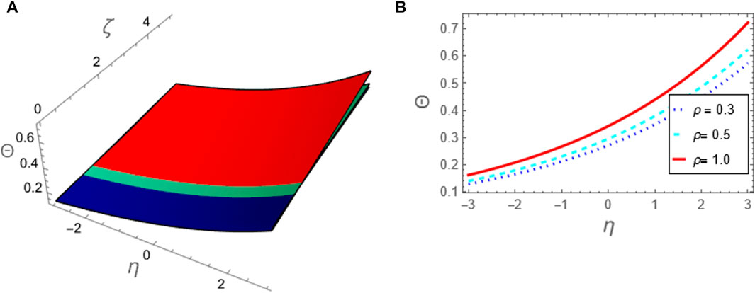
Figure 1. The approximation (49) to problem 1 using ARPSM is considered against the fractional parameter p: (A) The approximation (49) is plotted in (ζ, η)-plane and (B) The approximation (49) is plotted against η at (ζ = 5).

Figure 2

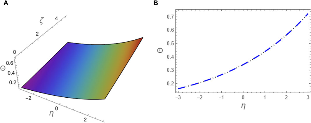
Figure 2. The approximation (49) to problem 1 using ARPSM at p = 1 is compared with the exact solution (39) for the integer case: (A) The two solutions are plotted in (ζ, η)-plane and (B) The two solutions are plotted against η at (ζ = 5).

Figure 3

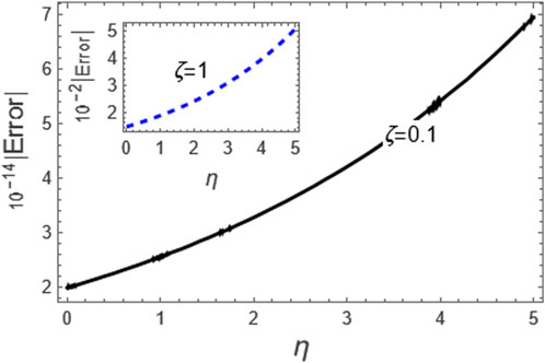
Figure 3. Here, we considered the absolute error of the approximation (49) as compared to the exact solution (39) for the integer case, i.e., p = 1.

Table 1

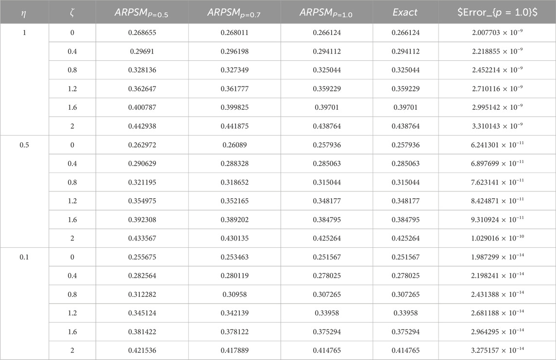
Table 1. The approximation (49) to problem 1 using ARPSM is considered against the fractional parameter p = 1.

Figure 4

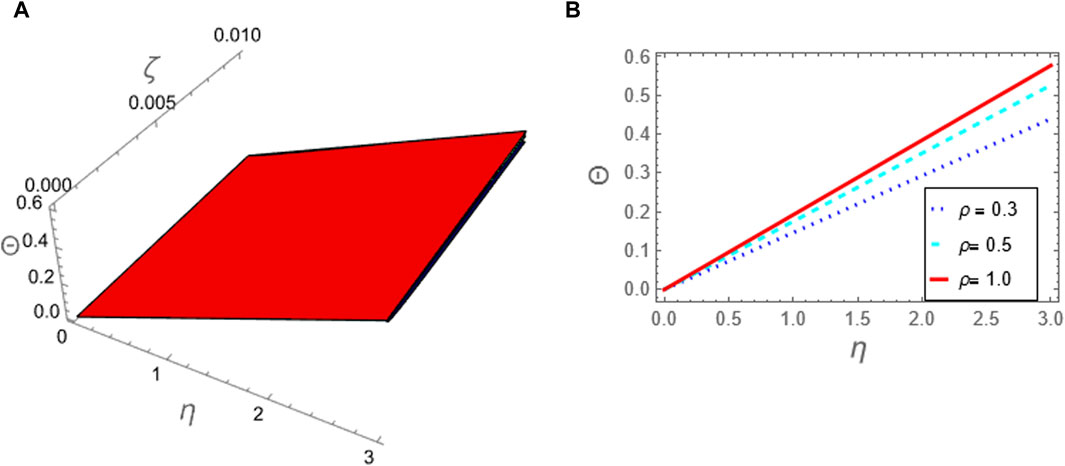
Figure 4. The approximation (61) to problem 2 using ARPSM is considered against the fractional parameter p: (A) The approximation (61) is plotted in (ζ, η)-plane and (B) The approximation (61) is plotted against η at (ζ = 0.1).

Figure 5

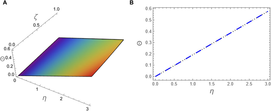
Figure 5. The approximation (61) to problem 2 using ARPSM at p = 1 is compared with the exact solution (52) for the integer case: (A) The two solutions are plotted in (ζ, η)-plane and (B) The two solutions are plotted against η at (ζ = 0.1).

Figure 6

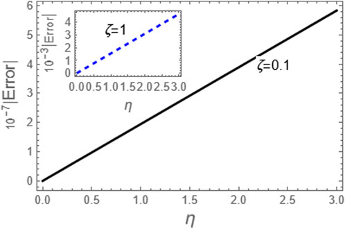
Figure 6. Here, we considered the absolute error of the approximation (61) as compared to the exact solution (52) for the integer case, i.e., p = 1.

Table 2

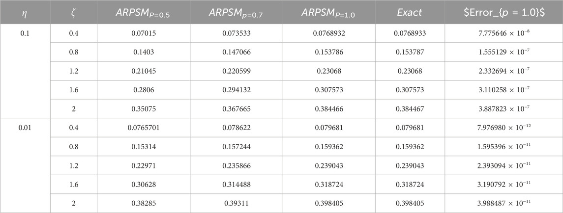
Table 2. The approximation (61) to problem 2 using ARPSM is considered against the fractional parameter.

3.4 Concept of the Aboodh transform iterative method (ATIM)

Let us consider a general PDE of fractional order in space-time.

D_{η}^{p} Θ (ζ, η) = Φ (Θ (ζ, η), D_{ζ}^{η} Θ (ζ, η), D_{ζ}^{2 η} Θ (ζ, η), D_{ζ}^{3 η} Θ (ζ, η)), 0 < p, η \leq 1, (62)

Initial conditions

Θ^{(k)} (ζ, 0) = h_{k}, k = 0,1,2, \dots, m - 1, (63)

Assuming Θ(ζ, η) as the unknown function, while $Φ (Θ (ζ, η), D_{ζ}^{η} Θ (ζ, η), D_{ζ}^{2 η} Θ (ζ, η) D_{ζ}^{3 η} Θ (ζ, η))$ may be a nonlinear or linear operator of $Θ (ζ, η), D_{ζ}^{η} Θ (ζ, η), D_{ζ}^{2 η} Θ (ζ, η)$ and $D_{ζ}^{3 η} Θ (ζ, η)$ . Applying the AT to both sides of Eq. 62 yields the following equation; Θ(ζ, η) is represented by Θ for simplicity.

A [Θ (ζ, η)] = \frac{1}{s^{p}} (\sum_{k = 0}^{m - 1} \frac{Θ^{(k)} (ζ, 0)}{s^{2 - p + k}} + A [Φ (Θ (ζ, η), D_{ζ}^{η} Θ (ζ, η), D_{ζ}^{2 η} Θ (ζ, η), D_{ζ}^{3 η} Θ (ζ, η))]), (64)

The problem may be solved by using the inverse of AT, which results in:

Θ (ζ, η) = A^{- 1} [\frac{1}{s^{p}} (\sum_{k = 0}^{m - 1} \frac{Θ^{(k)} (ζ, 0)}{s^{2 - p + k}} + A [Φ (Θ (ζ, η), D_{ζ}^{η} Θ (ζ, η), D_{ζ}^{2 η} Θ (ζ, η), D_{ζ}^{3 η} Θ (ζ, η))])] . (65)

An infinite series is used to represent the solution that is achieved by the iterative processing of the AT technique.

Θ (ζ, η) = \sum_{i = 0}^{\infty} Θ_{i} . (66)

Since $Φ (Θ, D_{ζ}^{η} Θ, D_{ζ}^{2 η} Θ, D_{ζ}^{3 η} Θ)$ is either a nonlinear or linear operator which can be decomposed as follows:

\begin{aligned} Φ (Θ, D_{ζ}^{η} Θ, D_{ζ}^{2 η} Θ, D_{ζ}^{3 η} Θ) = Φ (Θ_{0}, D_{ζ}^{η} Θ_{0}, D_{ζ}^{2 η} Θ_{0}, D_{ζ}^{3 η} Θ_{0}) \\ + \sum_{i = 0}^{\infty} (Φ (\sum_{k = 0}^{i} (Θ_{k}, D_{ζ}^{η} Θ_{k}, D_{ζ}^{2 η} Θ_{k}, D_{ζ}^{3 η} Θ_{k})) - Φ (\sum_{k = 1}^{i - 1} (Θ_{k}, D_{ζ}^{η} Θ_{k}, D_{ζ}^{2 η} Θ_{k}, D_{ζ}^{3 η} Θ_{k})) ) . \end{aligned} (67)

In order to derive the succeeding equation, it is necessary to substitute Eqs 67 and (66) into Eq. 65 to yield

\begin{aligned} \sum_{i = 0}^{\infty} Θ_{i} (ζ, η) = A^{- 1} [\frac{1}{s^{p}} (\sum_{k = 0}^{m - 1} \frac{Θ^{(k)} (ζ, 0)}{s^{2 - p + k}} + A [Φ (Θ_{0}, D_{ζ}^{η} Θ_{0}, D_{ζ}^{2 η} Θ_{0}, D_{ζ}^{3 η} Θ_{0})])] \\ + A^{- 1} [\frac{1}{s^{p}} (A [\sum_{i = 0}^{\infty} (Φ \sum_{k = 0}^{i} (Θ_{k}, D_{ζ}^{η} Θ_{k}, D_{ζ}^{2 η} Θ_{k}, D_{ζ}^{3 η} Θ_{k}))])] \\ - A^{- 1} [\frac{1}{s^{p}} (A [(Φ \sum_{k = 1}^{i - 1} (Θ_{k}, D_{ζ}^{η} Θ_{k}, D_{ζ}^{2 η} Θ_{k}, D_{ζ}^{3 η} Θ_{k}))])] \end{aligned} (68)

\begin{aligned} Θ_{0} (ζ, η) = A^{- 1} [\frac{1}{s^{p}} (\sum_{k = 0}^{m - 1} \frac{Θ^{(k)} (ζ, 0)}{s^{2 - p + k}})], \\ Θ_{1} (ζ, η) = A^{- 1} [\frac{1}{s^{p}} (A [Φ (Θ_{0}, D_{ζ}^{η} Θ_{0}, D_{ζ}^{2 η} Θ_{0}, D_{ζ}^{3 η} Θ_{0})])], \\ ⋮ \\ Θ_{m + 1} (ζ, η) = A^{- 1} [\frac{1}{s^{p}} (A [\sum_{i = 0}^{\infty} (Φ \sum_{k = 0}^{i} (Θ_{k}, D_{ζ}^{η} Θ_{k}, D_{ζ}^{2 η} Θ_{k}, D_{ζ}^{3 η} Θ_{k}))])] \\ - A^{- 1} [\frac{1}{s^{p}} (A [(Φ \sum_{k = 1}^{i - 1} (Θ_{k}, D_{ζ}^{η} Θ_{k}, D_{ζ}^{2 η} Θ_{k}, D_{ζ}^{3 η} Θ_{k}))])], m = 1,2, \dots . \end{aligned} (69)

Equation 62 may be stated in the following manner, which provides the analytically approximate solution for the m-term expression:

Θ (ζ, η) = \sum_{i = 0}^{m - 1} Θ_{i} . (70)

3.4.1 Anatomy Problem (1) using ATIM

Let us consider the following time fractional PDE [51]:

\begin{aligned} D_{η}^{p} Θ (ζ, η) = - Θ (ζ, η) \frac{\partial^{3} Θ (ζ, η)}{\partial ζ^{3}} + \frac{\partial Θ (ζ, η)}{\partial ζ} \frac{\partial^{2} Θ (ζ, η)}{\partial ζ^{2}} + \frac{\partial^{2} Θ (ζ, η)}{\partial ζ^{2}}, where 0 < p \leq 1 \end{aligned} (71)

with the following IC’s:

\begin{aligned} Θ (ζ, 0) = \frac{e^{ζ / 4}}{4}, \end{aligned} (72)

and the following exact solution

\begin{aligned} Θ (ζ, η) = \frac{1}{4} e^{\frac{1}{4} (\frac{η}{4} + ζ)} . \end{aligned} (73)

By using AT on both sides of Eq. 71, we get the following outcome:

A [D_{η}^{p} Θ (ζ, η)] = \frac{1}{s^{p}} (\sum_{k = 0}^{m - 1} \frac{Θ^{(k)} (ζ, 0)}{s^{2 - p + k}} + A [- Θ (ζ, η) \frac{\partial^{3} Θ (ζ, η)}{\partial ζ^{3}} + \frac{\partial Θ (ζ, η)}{\partial ζ} \frac{\partial^{2} Θ (ζ, η)}{\partial ζ^{2}} + \frac{\partial^{2} Θ (ζ, η)}{\partial ζ^{2}}]), (74)

In order to produce the following, we apply the inverse of AT on both sides of Eq. 74.

Θ (ζ, η) = A^{- 1} [\frac{1}{s^{p}} (\sum_{k = 0}^{m - 1} \frac{Θ^{(k)} (ζ, 0)}{s^{2 - p + k}} + A [- Θ (ζ, η) \frac{\partial^{3} Θ (ζ, η)}{\partial ζ^{3}} + \frac{\partial Θ (ζ, η)}{\partial ζ} \frac{\partial^{2} Θ (ζ, η)}{\partial ζ^{2}} + \frac{\partial^{2} Θ (ζ, η)}{\partial ζ^{2}} ] ) ] . (75)

The equation that we get by applying the AT in an iterative manner can be described as follows:

\begin{aligned} Θ_{0} (ζ, η) = & A^{- 1} [\frac{1}{s^{p}} (\sum_{k = 0}^{m - 1} \frac{Θ^{(k)} (ζ, 0)}{s^{2 - p + k}})] \\ = A^{- 1} [\frac{Θ (ζ, 0)}{s^{2}}] \\ = \frac{e^{ζ / 4}}{4}, \end{aligned}

Through the application of the RL integral to Eq. 71, we are able to get the equivalent form.

\begin{aligned} Θ (ζ, η) = \frac{e^{ζ / 4}}{4} - A [- Θ (ζ, η) \frac{\partial^{3} Θ (ζ, η)}{\partial ζ^{3}} + \frac{\partial Θ (ζ, η)}{\partial ζ} \frac{\partial^{2} Θ (ζ, η)}{\partial ζ^{2}} + \frac{\partial^{2} Θ (ζ, η)}{\partial ζ^{2}}] . \end{aligned} (76)

Utilizing the ATIM, the following are some of the terms that may be obtained:

\begin{aligned} Θ_{0} (ζ, η) = \frac{e^{ζ / 4}}{4}, \\ Θ_{1} (ζ, η) = \frac{e^{ζ / 4} η^{p}}{64 Γ (p + 1)}, \\ Θ_{2} (ζ, η) = \frac{\sqrt{π} 4^{- p - 5} e^{ζ / 4} η^{2 p}}{Γ (p + \frac{1}{2}) Γ (p + 1)}, \\ Θ_{3} (ζ, η) = \frac{e^{ζ / 4} η^{3 p}}{16384 Γ (3 p + 1)}, \\ Θ_{4} (ζ, η) = \frac{e^{ζ / 4} η^{4 p}}{262144 p Γ (p) Γ (3 p + 1)}, \end{aligned} (77)

The final approximation is obtained as follows:

\begin{aligned} Θ (ζ, η) = Θ_{0} (ζ, η) + Θ_{1} (ζ, η) + Θ_{2} (ζ, η) + Θ_{3} (ζ, η) + \dots . \end{aligned} (78)

\begin{aligned} Θ (ζ, η) = & \frac{e^{ζ / 4} η^{p}}{64 Γ (p + 1)} + \frac{\sqrt{π} 4^{- p - 5} e^{ζ / 4} η^{2 p}}{Γ (p + \frac{1}{2}) Γ (p + 1)} + \frac{e^{ζ / 4} η^{3 p}}{16384 Γ (3 p + 1)} \\ + \frac{e^{ζ / 4} η^{4 p}}{262144 p Γ (p) Γ (3 p + 1)} + \dots . \end{aligned} (79)

3.4.2 Anatomy Problem (2) using ATIM

Let us considered the following time fractional damped nonlinear Burger’s equation [51]:

\begin{aligned} D_{η}^{p} Θ (ζ, η) = - \frac{\partial^{2} Θ (ζ, η)}{\partial x^{2}} - Θ (ζ, η) \frac{\partial Θ (ζ, η)}{\partial x} - \frac{1}{5} Θ (ζ, η), where 0 < p \leq 1 \end{aligned} (80)

with the following IC’s:

\begin{aligned} Θ (ζ, 0) = \frac{1}{5} ζ, \end{aligned} (81)

and the following exact solution

\begin{aligned} Θ (ζ, η) = \frac{ζ}{5 (2 e^{\frac{η}{5}} - 1)} . \end{aligned} (82)

The application of AT to either side of Eq. 80, we are able to get the following equation:

\begin{aligned} A [D_{η}^{p} Θ (ζ, η)] = \frac{1}{s^{p}} (\sum_{k = 0}^{m - 1} \frac{Θ^{(k)} (ζ, 0)}{s^{2 - p + k}} + A [- \frac{\partial^{2} Θ (ζ, η)}{\partial x^{2}} - Θ (ζ, η) \frac{\partial Θ (ζ, η)}{\partial x} - \frac{1}{5} Θ (ζ, η)  ]), \end{aligned} (83)

Applying the inverse of AT to Eq. 83 yields

\begin{aligned} Θ (ζ, η) = A^{- 1} [\frac{1}{s^{p}} (\sum_{k = 0}^{m - 1} \frac{Θ^{(k)} (ζ, 0)}{s^{2 - p + k}} + A [- \frac{\partial^{2} Θ (ζ, η)}{\partial x^{2}} - Θ (ζ, η) \frac{\partial Θ (ζ, η)}{\partial x} - \frac{1}{5} Θ (ζ, η)])] . \end{aligned} (84)

Using the iterative procedure of AT, we get

\begin{aligned} Θ_{0} (ζ, η) = & A^{- 1} [\frac{1}{s^{p}} (\sum_{k = 0}^{m - 1} \frac{Θ^{(k)} (ζ, 0)}{s^{2 - p + k}})] \\ = A^{- 1} [\frac{Θ (ζ, 0)}{s^{2}}] \\ = \frac{1}{5} ζ, \end{aligned}

Using the RL integral results in the equivalent form being obtained from Eq. 50.

\begin{aligned} Θ (ζ, η) = \frac{1}{5} ζ - A [- \frac{\partial^{2} Θ (ζ, η)}{\partial x^{2}} - Θ (ζ, η) \frac{\partial Θ (ζ, η)}{\partial x} - \frac{1}{5} Θ (ζ, η)] . \end{aligned} (85)

The ATIM resulted in the following few terms being produced.

\begin{aligned} Θ_{0} (ζ, η) = \frac{1}{5} ζ, \\ Θ_{1} (ζ, η) = - \frac{2 ζ η^{p}}{25 Γ (p + 1)}, \\ Θ_{2} (ζ, η) = \frac{2 ζ η^{2 p} (15 - \frac{2 η^{p} Γ {(2 p + 1)}^{2}}{Γ {(p + 1)}^{2} Γ (3 p + 1)})}{625 Γ (2 p + 1)}, \\ Θ_{3} (ζ η) = \frac{2 ζ η^{3 p}}{390625} (2 η^{p} (- \frac{4 η^{3 p} Γ {(2 p + 1)}^{2} Γ (6 p + 1)}{Γ {(p + 1)}^{4} Γ {(3 p + 1)}^{2} Γ (7 p + 1)} + \frac{\frac{60 η^{2 p} Γ (5 p + 1)}{Γ (3 p + 1) Γ (6 p + 1)} + \frac{125 \sqrt{π} 2^{- 4 p}}{Γ (2 p + \frac{1}{2})}}{Γ {(p + 1)}^{2}} \\ - \frac{225 η^{p} Γ (4 p + 1)}{Γ {(2 p + 1)}^{2} Γ (5 p + 1)} - \frac{100 η^{p} Γ (2 p + 1) Γ (4 p + 1)}{Γ {(p + 1)}^{3} Γ (3 p + 1) Γ (5 p + 1)} + \frac{750 Γ (3 p + 1)}{Γ (p + 1) Γ (2 p + 1) Γ (4 p + 1)}) - \frac{1875}{Γ (3 p + 1)}), \end{aligned} (86)

We finally get

\begin{aligned} Θ (ζ, η) = Θ_{0} (ζ, η) + Θ_{1} (ζ, η) + Θ_{2} (ζ, η) + Θ_{3} (ζ, η) + \dots \end{aligned} (87)

\begin{aligned} Θ (ζ, η) = \frac{1}{5} ζ - \frac{2 ζ η^{p}}{25 Γ (p + 1)} + \frac{2 ζ η^{2 p} (15 - \frac{2 η^{p} Γ {(2 p + 1)}^{2}}{Γ {(p + 1)}^{2} Γ (3 p + 1)})}{625 Γ (2 p + 1)} \\ + \frac{2 ζ η^{3 p}}{390625} (2 η^{p} (- \frac{4 η^{3 p} Γ {(2 p + 1)}^{2} Γ (6 p + 1)}{Γ {(p + 1)}^{4} Γ {(3 p + 1)}^{2} Γ (7 p + 1)} + \frac{\frac{60 η^{2 p} Γ (5 p + 1)}{Γ (3 p + 1) Γ (6 p + 1)} + \frac{125 \sqrt{π} 2^{- 4 p}}{Γ (2 p + \frac{1}{2})}}{Γ {(p + 1)}^{2}} \\ - \frac{225 η^{p} Γ (4 p + 1)}{Γ {(2 p + 1)}^{2} Γ (5 p + 1)} - \frac{100 η^{p} Γ (2 p + 1) Γ (4 p + 1)}{Γ {(p + 1)}^{3} Γ (3 p + 1) Γ (5 p + 1)} + \frac{750 Γ (3 p + 1)}{Γ (p + 1) Γ (2 p + 1) Γ (4 p + 1)}) - \frac{1875}{Γ (3 p + 1)}) . \end{aligned} (88)

Here, we graphically and numerically analyzed the derived approximations (79) and (88) using AITM for problems 1 and 2, respectively, as illustrated in Figures 7–12; Tables 3, 4. These figures demonstrate the impact of the fractional parameter p on the behavior of the wave described by this approximation and the absolute errors for these approximations as compared to the exact solutions for the integer case. We can observe the effect of the fractional parameter on the behavior of the deduced approximations and the accuracy and stability of these approximations along the study domain. This is one of the most essential features of AITM, which gives more accurate and stable approximations throughout the study domain. In the last part, we discussed comparing the approximations derived by ARPSM and those derived by AITM, as evident in Tables 5, 6. It is observed from the comparison results that both approaches give more accurate and stable approximations throughout the study domain, but ARPSM differs somewhat in its accuracy from AITM, i.e., the derived approximations using ARPSM are more accurate than AITM.

Figure 7

Figure 7. The approximation (79) to problem 1 using ATIM is considered against the fractional parameter p: (A) The approximation (79) is plotted in (ζ, η)-plane and (B) The approximation (79) is plotted against η for (ζ = 5).

Figure 8

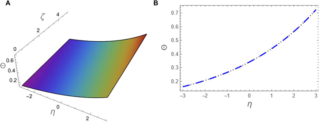
Figure 8. The approximation (79) to problem 1 using ATIM at p = 1 is compared with the exact solution (73) for the integer case: (A) The two solutions are plotted in (ζ, η)-plane and (B) The two solutions are plotted against η at (ζ = 5).

Figure 9

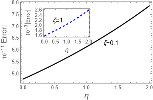
Figure 9. Here, we considered the absolute error of the approximation (79) as compared to the exact solution (73) for the integer case, i.e., p = 1.

Figure 10

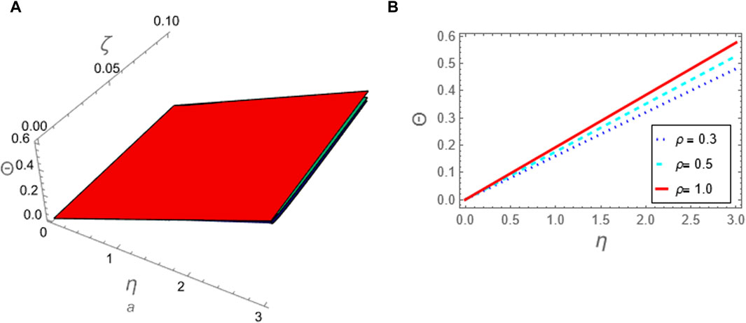
Figure 10. The approximation (88) to problem 2 using ATIM is considered against the fractional parameter p: (A) The approximation (88) is plotted in (ζ, η)-plane and (B) The approximation (88) is plotted against η at (ζ = 0.1).

Figure 11

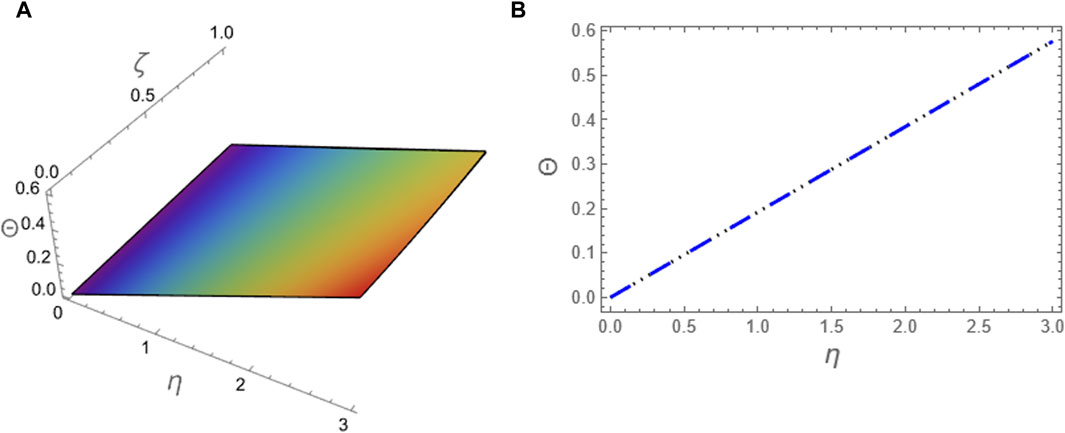
Figure 11. The approximation (88) to problem 2 using ATIM at p = 1 is compared with the exact solution (83) for the integer case: (A) The two solutions are plotted in (ζ, η)-plane and (B) The two solutions are plotted against η at (ζ = 0.1).

Figure 12

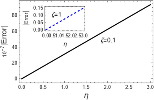
Figure 12. Here, we considered the absolute error of the approximation (88) as compared to the exact solution (83) for the integer case, i.e., p = 1.

Table 3

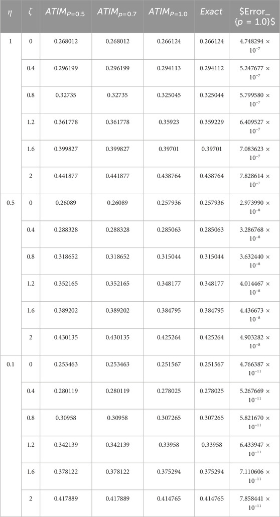
Table 3. The approximation (79) of problem 1 using AITM is considered against the fractional parameter.

Table 4

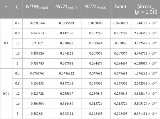
Table 4. The approximation (88) of problem 2 using ATIM is numerically against the fractional parameter p.

Table 5

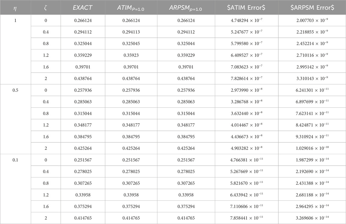
Table 5. The absolute error between the derived approximations and the exact solutions for the integer cases (p = 1) is compared for both NITM and APRSM, for problem 1.

Table 6

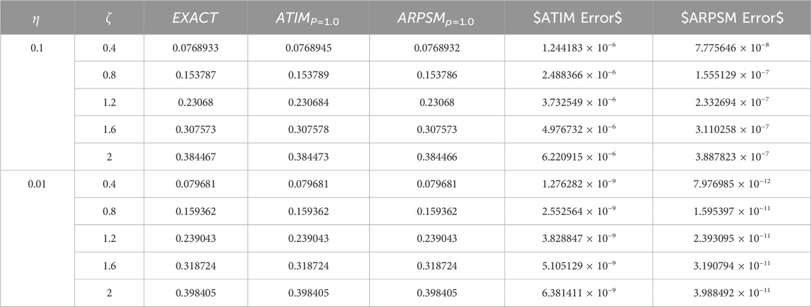
Table 6. The absolute error between the derived approximations and the exact solutions for the integer cases (p = 1) is compared for both NITM and APRSM, for problem 2.

4 Conclusion

The damped Burger’s equation and many other associated equations with the dissipative term arise in plasma physics due to taking the viscosity force in the fluid equations that govern a plasma model. On the other side, the damped effect occurs due to considering the collisional effect between the charged plasma particles. Motivated by these applications, thus, this study analyzed this equation by employing advanced mathematical techniques known as the Aboodh residual power series method (ARPSM) and the Aboodh transform iteration method (ATIM). The fractional derivatives were processed using the Caputo operator. The use of this operator is due to its ability to enrich modeling by considering fractional derivatives, which contributes to a more accurate representation of the fundamental dynamics of the equations under study. We have derived a set of precise highly approximations using the suggested strategies. The derived approximations have been analyzed and examined graphically and numerically by plotting some two- and three-dimensional graphics. Moreover, we discussed the obtained approximations numerically in some suitable tables and estimated the absolute errors compared to the exact solutions for the integer cases. The suggested methods proved effective for getting highly accurate and more stable approximations of more complicated fractional differential equations. Moreover, the obtained results demonstrated the high accuracy, efficiency, and rapid calculations of the suggested methods in analyzing damped Burger’s equation. The comparison results between the obtained approximations using ARPSM and AITM demonstrated that the derived approximations using ARPSM are more accurate than AITM.

The study offers valuable insights into the dynamic behavior of solutions to Damped Burger’s equation, demonstrating the effectiveness of the suggested strategies in dealing with the difficulties presented by nonlinear fractional partial differential equations. This inquiry enhances mathematical modeling and numerical analysis by highlighting the effectiveness of ARPSM and ATIM in solving intricate equations in different scientific fields. Therefore, it is expected that the results of this study will serve many physics researchers interested in the field of plasma physics, fluids, electronics, and optical fibers to study the characteristics of nonlinear phenomena that arise and propagate in these physical systems.

5 Future work

The suggested approaches can be used in analyzing many strong nonlinear and more complicated evolution equations that are derived from the fluid equations to some plasma models, such as KdV-type equations with third-order dispersion [52–54], Burger’s-type equations [55–57], Kawahara-type equations with fifth-order dispersion [58–60], nonlinear Schrödinger-type equations [61, 62], and many other evolution equations. Therefore, the characteristics of the many nonlinear phenomena that can be generated and propagated in various plasma systems can be accurately described and examined by studying the effect of the fractional parameters on the behavior of these phenomena, such as solitons, dissipative solitons, shocks, dissipative shocks, rogue waves, dissipative rogue waves, periodic waves, dissipative periodic waves, etc., which are among the most famous phenomena that spread in multicomponent plasmas.

Data availability statement

The original contributions presented in the study are included in the article/Supplementary material, further inquiries can be directed to SE-T.

Author contributions

SN: Conceptualization, Data curation, Formal Analysis, Writing–original draft. WA: Project administration, Software, Supervision, Writing–review and editing. RS: Data curation, Funding acquisition, Investigation, Resources, Writing–original draft. MA-S: Investigation, Methodology, Project administration, Writing–review and editing. SI: Investigation, Resources, Supervision, Writing–review and editing. SE-T: Formal Analysis, Investigation, Methodology, Resources, Software, Supervision, Validation, Writing–review and editing.

Funding

The author(s) declare that financial support was received for the research, authorship, and/or publication of this article. This work was supported by the Deanship of Scientific Research, Vice Presidency for Graduate Studies and Scientific Research, King Faisal University, Saudi Arabia (Grant No. 6074). This study was supported via funding from Prince Sattam bin Abdulaziz University project number (PSAU/2024/R/1445).

Acknowledgments

The authors express their gratitude to Princess Nourah bintAbdulrahman University Researchers Supporting Project Number (PNURSP2024R157), Princess Nourah bint Abdul Rahman University, Riyadh, Saudi Arabia. This work was supported by the Deanship of Scientific Research, Vice Presidency for Graduate Studies and Scientific Research, King Faisal University, Saudi Arabia (Grant No. 6074).

Conflict of interest

The authors declare that the research was conducted in the absence of any commercial or financial relationships that could be construed as a potential conflict of interest.

Publisher’s note

All claims expressed in this article are solely those of the authors and do not necessarily represent those of their affiliated organizations, or those of the publisher, the editors and the reviewers. Any product that may be evaluated in this article, or claim that may be made by its manufacturer, is not guaranteed or endorsed by the publisher.

References

1. Podlubny I. Mathematics in science and engineering fractional differential equations: an introduction to fractional derivatives, fractional differential equations, to methods of their solution and some of their applications. San Diego: Academic Press (1999).

Google Scholar

2. Sene N. Stokes’ first problem for heated flat plate with Atangana-Baleanu fractional derivative. Chaos, Solitons and Fractals (2018) 117:68–75. doi:10.1016/j.chaos.2018.10.014

CrossRef Full Text | Google Scholar

3. Zhang L, Kwizera S, Khalique CM. A study of a new genralized Burgers equatio: symmetry solutions and conservation Laws. Adv Math Models Appl (2023) 8(2).

Google Scholar

4. Jafari H, Ganji RM, Ganji DD, Hammouch Z, Gasimov YS. A novel numerical method for solving fuzzy variable-order differential equations with Mittag-Leffler kernels. Fractals (2023) 31:2340063. doi:10.1142/s0218348x23400637

CrossRef Full Text | Google Scholar

5. Gasimov YS, Napoles-Vald JE. Some refinements of hermite hadamard inequality using K-fractional Caputo derivatives. Fractional Differential Calculus (2022) 12(2):209–21. doi:10.7153/fdc-2022-12-13

CrossRef Full Text | Google Scholar

6. Salati S, Matinfar M, Jafari H. A numerical approach for solving Bagely-Torvik and fractional oscillation equations. Adv Math Model Appl (2023) 8(2):241–52.

Google Scholar

7. Ahmad S, Ullah A, Shah K, Akgul A. Computational analysis of the third order dispersive fractional PDE under exponential decay and Mittag Leffler type kernels. Numer Methods Partial Differential Equations (2023) 39(6):4533–48. doi:10.1002/num.22627

CrossRef Full Text | Google Scholar

8. Qureshi S, Yusuf A, Ali Shaikh A, Inc M, Baleanu D. Mathematical modeling for adsorption process of dye removal nonlinear equation using power law and exponentially decaying kernels. Chaos: Interdiscip J Nonlinear Sci (2020) 30(4):043106. doi:10.1063/1.5121845

PubMed Abstract | CrossRef Full Text | Google Scholar

9. Ahmad S, Ullah A, Arfan M, Shah K. On analysis of the fractional mathematical model of rotavirus epidemic with the effects of breastfeeding and vaccination under Atangana-Baleanu (AB) derivative. Chaos, Solitons and Fractals (2020) 140:110233. doi:10.1016/j.chaos.2020.110233

CrossRef Full Text | Google Scholar

10. Ullah A, Abdeljawad T, Ahmad S, Shah K. Study of a fractional-order epidemic model of childhood diseases. J Funct Spaces (2020) 2020:1–8. doi:10.1155/2020/5895310

CrossRef Full Text | Google Scholar

11. Qureshi S, Yusuf A, Shaikh AA, Inc M, Baleanu D. Fractional modeling of blood ethanol concentration system with real data application. Chaos: Interdiscip J Nonlinear Sci (2019) 29(1):013143. doi:10.1063/1.5082907

PubMed Abstract | CrossRef Full Text | Google Scholar

12. Caputo M, Fabrizio M. A new definition of fractional derivative without singular kernel. Prog Fractional Differ Appl (2015) 1(2):73–85.

Google Scholar

13. Dokuyucu MA. A fractional order alcoholism model via Caputo-Fabrizio derivative. Aims Math (2020) 5(2):781–97. doi:10.3934/math.2020053

CrossRef Full Text | Google Scholar

14. Alizadeh S, Baleanu D, Rezapour S. Analyzing transient response of the parallel RCL circuit by using the Caputo-Fabrizio fractional derivative. Adv Difference Equations (2020) 2020:55–19. doi:10.1186/s13662-020-2527-0

CrossRef Full Text | Google Scholar

15. Higazy M, Alyami MA. New Caputo-Fabrizio fractional order SEIASqEqHR model for COVID-19 epidemic transmission with genetic algorithm based control strategy. Alexandria Eng J (2020) 59(6):4719–36. doi:10.1016/j.aej.2020.08.034

CrossRef Full Text | Google Scholar

16. Guo C, Hu J, Hao J, Celikovsky S, Hu X. Fixed-time safe tracking control of uncertain high-order nonlinear pure-feedback systems via unified transformation functions. Kybernetika (2023) 59(3):342–64. doi:10.14736/kyb-2023-3-0342

CrossRef Full Text | Google Scholar

17. Guo C, Hu J, Wu Y, Celikovsky S. Non-singular fixed-time tracking control of uncertain nonlinear pure-feedback systems with practical state constraints. IEEE Trans Circuits Syst Regular Pap (2023) 70(9):3746–58. doi:10.1109/TCSI.2023.3291700

CrossRef Full Text | Google Scholar

18. Lu Z, Yang T, Brennan MJ, Liu Z, Chen L. Experimental investigation of a two-stage nonlinear vibration isolation system with high-static-low-dynamic stiffness. J Appl Mech (2016) 84(2). doi:10.1115/1.4034989

CrossRef Full Text | Google Scholar

19. Lu Z, Brennan M, Ding H, Chen L. High-static-low-dynamic-stiffness vibration isolation enhanced by damping nonlinearity. Sci China Technol Sci (2018) 62:1103–10. doi:10.1007/s11431-017-9281-9

CrossRef Full Text | Google Scholar

20. Luo R, Peng Z, Hu J, Ghosh BK. Adaptive optimal control of affine nonlinear systems via identifier-critic neural network approximation with relaxed PE conditions. Neural Networks (2023) 167:588–600. doi:10.1016/j.neunet.2023.08.044

PubMed Abstract | CrossRef Full Text | Google Scholar

21. Kai Y, Chen S, Zhang K, Yin Z. Exact solutions and dynamic properties of a nonlinear fourth-order time-fractional partial differential equation. Waves in Random and Complex Media (2022) 2022:2044541–12. doi:10.1080/17455030.2022.2044541

CrossRef Full Text | Google Scholar

22. Gao J, Liu J, Yang H, Liu H, Zeng G, Huang B. Anisotropic medium sensing controlled by bound states in the continuum in polarization-independent metasurfaces. Opt Express (2023) 31(26):44703–19. doi:10.1364/OE.509673

PubMed Abstract | CrossRef Full Text | Google Scholar

23. Bai X, He Y, Xu M. Low-thrust reconfiguration strategy and optimization for formation flying using Jordan normal form. IEEE Trans Aerospace Electron Syst (2021) 57(5):3279–95. doi:10.1109/TAES.2021.3074204

CrossRef Full Text | Google Scholar

24. Li Y, Kai Y. Wave structures and the chaotic behaviors of the cubic-quartic nonlinear Schrodinger equation for parabolic law in birefringent fibers. Nonlinear Dyn (2023) 111(9):8701–12. doi:10.1007/s11071-023-08291-3

CrossRef Full Text | Google Scholar

25. Zhou X, Liu X, Zhang G, Jia L, Wang X, Zhao Z. An iterative threshold algorithm of log-sum regularization for sparse problem. IEEE Trans Circuits Syst Video Tech (2023) 33(9):4728–40. doi:10.1109/TCSVT.2023.3247944

CrossRef Full Text | Google Scholar

26. Wang R, Feng Q, Ji J. The discrete convolution for fractional cosine-sine series and its application in convolution equations. AIMS Math (2024) 9(2):2641–56. doi:10.3934/math.2024130

CrossRef Full Text | Google Scholar

27. Yasmin H, Aljahdaly NH, Saeed AM, Shah R. Investigating symmetric soliton solutions for the fractional coupled konno-onno system using improved versions of a novel analytical technique. Mathematics (2023) 11(12):2686. doi:10.3390/math11122686

CrossRef Full Text | Google Scholar

28. Watugala GK. (1992). Sumudu transform-a new integral transform to solve differential equations and control engineering problems. in Control 92: Enhancing Australia’s Productivity Through Automation, Control and Instrumentation; Preprints of Papers, Barton, ACT, 01 January 1992, (Australia: Institution of Engineers) 245–59.

Google Scholar

29. Elzaki TM. Application of new transform “Elzaki transform” to partial differential equations. Glob J Pure Appl Math (2011) 7(1):65–70.

Google Scholar

30. Aboodh KS. Application of new transform “Aboodh Transform” to partial differential equations. Glob J Pure Appl Math (2014) 10(2):249–54.

Google Scholar

31. Arqub OA. Series solution of fuzzy differential equations under strongly generalized differentiability. J Adv Res Appl Math (2013) 5(1):31–52. doi:10.5373/jaram.1447.051912

CrossRef Full Text | Google Scholar

32. Mukhtar S, Shah R, Noor S. The numerical investigation of a fractional-order multi-dimensional Model of Navier-Stokes equation via novel techniques. Symmetry (2022) 14(6):1102. doi:10.3390/sym14061102

CrossRef Full Text | Google Scholar

33. Arqub OA, El-Ajou A, Zhour ZA, Momani S. Multiple solutions of nonlinear boundary value problems of fractional order: a new analytic iterative technique. Entropy (2014) 16(1):471–93. doi:10.3390/e16010471

CrossRef Full Text | Google Scholar

34. El-Ajou A, Arqub OA, Momani S. Approximate analytical solution of the nonlinear fractional KdV-Burgers equation: a new iterative algorithm. J Comput Phys (2015) 293:81–95. doi:10.1016/j.jcp.2014.08.004

CrossRef Full Text | Google Scholar

35. Xu F, Gao Y, Yang X, Zhang H. Construction of fractional power series solutions to fractional Boussinesq equations using residual power series method. Math Probl Eng (2016) 2016:1–15. doi:10.1155/2016/5492535

CrossRef Full Text | Google Scholar

36. Saad Alshehry A, Imran M, Khan A, Weera W. Fractional view analysis of kuramoto-sivashinsky equations with non-singular kernel operators. Symmetry (2022) 14(7):1463. doi:10.3390/sym14071463

CrossRef Full Text | Google Scholar

37. Jaradat I, Alquran M, Abdel-Muhsen R. An analytical framework of 2D diffusion, wave-like, telegraph, and Burgers’ models with twofold Caputo derivatives ordering. Nonlinear Dyn (2018) 93:1911–22. doi:10.1007/s11071-018-4297-8

CrossRef Full Text | Google Scholar

38. Al-Sawalha MM, Shah R, Khan A, Ababneh OY, Botmart T. Fractional view analysis of Kersten-Krasil’shchik coupled KdV-mKdV systems with non-singular kernel derivatives. AIMS Math (2022) 7:18334–59. doi:10.3934/math.20221010

CrossRef Full Text | Google Scholar

39. Alderremy AA, Iqbal N, Aly S, Nonlaopon K. Fractional series solution construction for nonlinear fractional reaction-diffusion brusselator model utilizing laplace residual power series. Symmetry (2022) 14(9):1944. doi:10.3390/sym14091944

CrossRef Full Text | Google Scholar

40. Zhang MF, Liu YQ, Zhou XS. Efficient homotopy perturbation method for fractional non-linear equations using Sumudu transform. Therm Sci (2015) 19(4):1167–71. doi:10.2298/tsci1504167z

CrossRef Full Text | Google Scholar

41. Awuya MA, Subasi D. Aboodh transform iterative method for solving fractional partial differential equation with mittag–leffler kernel. Symmetry (2021) 13:2055. doi:10.3390/sym13112055

CrossRef Full Text | Google Scholar

42. Ojo GO, Mahmudov NI. Aboodh transform iterative method for spatial diffusion of a biological population with fractional-order. Mathematics (2021) 9:155. doi:10.3390/math9020155

CrossRef Full Text | Google Scholar

43. Awuya MA, Ojo GO, Mahmudov NI. Solution of space-time fractional differential equations using Aboodh transform iterative metho. J Math (2022) 2022:4861588. doi:10.1155/2022/4861588

CrossRef Full Text | Google Scholar

44. Liaqat MI, Etemad S, Rezapour S, Park C. A novel analytical Aboodh residual power series method for solving linear and nonlinear time-fractional partial differential equations with variable coefficients. AIMS Math (2022) 7(9):16917–48. doi:10.3934/math.2022929

CrossRef Full Text | Google Scholar

45. Liaqat MI, Akgul A, Abu-Zinadah H. Analytical investigation of some time-fractional black-scholes models by the Aboodh residual power series method. Mathematics (2023) 11(2):276. doi:10.3390/math11020276

CrossRef Full Text | Google Scholar

46. Aboodh KS. The new integral Transform’Aboodh transform. Glob J Pure Appl Math (2013) 9(1):35–43.

Google Scholar

47. Aggarwal S, Chauhan R. A comparative study of Mohand and Aboodh transforms. Int J Res advent Tech (2019) 7(1):520–9. doi:10.32622/ijrat.712019107

CrossRef Full Text | Google Scholar

48. Benattia ME, Belghaba K. Application of the Aboodh transform for solving fractional delay differential equations. Universal J Math Appl (2020) 3(3):93–101. doi:10.32323/ujma.702033

CrossRef Full Text | Google Scholar

49. Delgado BB, Macias-Diaz JE. On the general solutions of some non-homogeneous Div-curl systems with Riemann-Liouville and Caputo fractional derivatives. Fractal and Fractional (2021) 5(3):117. doi:10.3390/fractalfract5030117

CrossRef Full Text | Google Scholar

50. Alshammari S, Al-Smadi M, Hashim I, Alias MA. Residual power series technique for simulating fractional bagley-torvik problems emerging in applied physics. Appl Sci (2019) 9(23):5029. doi:10.3390/app9235029

CrossRef Full Text | Google Scholar

51. Acan O, Firat O, Keskin Y. Conformable variational iteration method, conformable fractional reduced differential transform method and conformable homotopy analysis method for non-linear fractional partial differential equations. Waves in Random and Complex Media (2020) 30(2):250–68. doi:10.1080/17455030.2018.1502485

CrossRef Full Text | Google Scholar

52. Almutlak SA, Parveen S, Mahmood S, Qamar A, Alotaibi BM, El-Tantawy SA. On the propagation of cnoidal wave and overtaking collision of slow shear Alfvén solitons in low β − magnetized plasmas. Phys Fluids (2023) 35:075130. doi:10.1063/5.0158292

CrossRef Full Text | Google Scholar

53. Hashmi T, Jahangir R, Masood W, Alotaibi BM, Ismaeel SME, El-Tantawy SA. Head-on collision of ion-acoustic (modified) Korteweg–de Vries solitons in Saturn’s magnetosphere plasmas with two temperature superthermal electrons. Phys Fluids (2023) 35:103104. doi:10.1063/5.0171220

CrossRef Full Text | Google Scholar

54. Batool N, Masood W, Siddiq M, Alrowaily AW, Ismaeel SME, El-Tantawy SA. Hirota bilinear method and multi-soliton interaction of electrostatic waves driven by cubic nonlinearity in pair-ion-electron plasmas. Phys Fluids (2023) 35:033109. doi:10.1063/5.0142447

CrossRef Full Text | Google Scholar

55. Wazwaz A-M, Alhejaili W, El-Tantawy SA. Physical multiple shock solutions to the integrability of linear structures of Burgers hierarchy. Phys Fluids (2023) 35:123101. doi:10.1063/5.0177366

CrossRef Full Text | Google Scholar

56. El-Tantawy SA, Matoog RT, Shah R, Alrowaily AW, Sherif ME. On the shock wave approximation to fractional generalized Burger–Fisher equations using the residual power series transform method. Phys Fluids (2024) 36:023105. doi:10.1063/5.0187127

CrossRef Full Text | Google Scholar

57. Aljahdaly NH, El-Tantawy SA, Wazwaz A-M, Ashi HA. Novel solutions to the undamped and damped KdV-Burgers-Kuramoto equations and modeling the dissipative nonlinear structures in nonlinear media. Rom Rep Phys (2022) 74:102

Google Scholar

58. Alkhateeb SA, Hussain S, Albalawi W, El-Tantawy SA, El-Awady EI. Dissipative Kawahara ion-acoustic solitary and cnoidal waves in a degenerate magnetorotating plasma. J Taibah Univ Sci (2023) 17(1):2187606. doi:10.1080/16583655.2023.2187606

CrossRef Full Text | Google Scholar

59. Alharbey RA, Alrefae WR, Malaikah H, Tag-Eldin E, El-Tantawy SA. Novel approximate analytical solutions to the nonplanar modified Kawahara equation and modeling nonlinear structures in electronegative plasmas. Symmetry (2023) 15(1):97. doi:10.3390/sym15010097

CrossRef Full Text | Google Scholar

60. Alharthi MR, Alharbey RA, El-Tantawy SA. Novel analytical approximations to the nonplanar Kawahara equation and its plasma applications. Eur Phys J Plus (2022) 137:1172. doi:10.1140/epjp/s13360-022-03355-6

CrossRef Full Text | Google Scholar

61. Irshad M, Rahman A, Khalid M, Khan S, Alotaibi BM, El-Sherif LS, et al. Effect of deformed Kaniadakis distribution on the modulational instability of electron-acoustic waves in a non-Maxwellian plasma. Phys Fluids (2023) 35:105116. doi:10.1063/5.0171327

CrossRef Full Text | Google Scholar

62. El-Tantawy SA, Aboelenen T. Simulation study of planar and nonplanar super rogue waves in an electronegative plasma: local discontinuous Galerkin method. Phys Plasmas (2017) 24:052118. doi:10.1063/1.4983327

CrossRef Full Text | Google Scholar

Keywords: nonlinear fractional partial differential equations (PDEs), damped Burger’s equation, Aboodh residual power series method, Aboodh transform iteration method, Caputo operator

Citation: Noor S, Albalawi W, Shah R, Al-Sawalha MM, Ismaeel SME and El-Tantawy SA (2024) On the approximations to fractional nonlinear damped Burger’s-type equations that arise in fluids and plasmas using Aboodh residual power series and Aboodh transform iteration methods. Front. Phys. 12:1374481. doi: 10.3389/fphy.2024.1374481

Received: 22 January 2024; Accepted: 04 March 2024;
Published: 02 April 2024.

Edited by:

Marina Chugunova, Claremont Graduate University, United States

Reviewed by:

Ahmad Qazza, Zarqa University, Jordan
Yusif Gasimov, Azerbaijan University, Azerbaijan

Copyright © 2024 Noor, Albalawi, Shah, Al-Sawalha, Ismaeel and El-Tantawy. This is an open-access article distributed under the terms of the Creative Commons Attribution License (CC BY). The use, distribution or reproduction in other forums is permitted, provided the original author(s) and the copyright owner(s) are credited and that the original publication in this journal is cited, in accordance with accepted academic practice. No use, distribution or reproduction is permitted which does not comply with these terms.

*Correspondence: Saima Noor, snoor@kfu.edu.sa; Rasool Shah, rasool.shah@lau.edu.lb

ORIGINAL RESEARCH article

On the approximations to fractional nonlinear damped Burger’s-type equations that arise in fluids and plasmas using Aboodh residual power series and Aboodh transform iteration methods

1 Introduction

2 Fundamental concepts

3 A route map describing the methods

3.1 Solving time-fractional PDEs with variable coefficients by use of the ARPSM process

3.2 Problem 1

3.3 Problem 2

3.4 Concept of the Aboodh transform iterative method (ATIM)

3.4.1 Anatomy Problem (1) using ATIM

3.4.2 Anatomy Problem (2) using ATIM

4 Conclusion

5 Future work

Data availability statement

Author contributions

Funding

Acknowledgments

Conflict of interest

Publisher’s note

References

This article is part of the Research Topic

People also looked at