


1. Introduction
The velocity gradient (VG) evolution in incompressible turbulent flows depends upon four fundamental processes: inertial, pressure, viscous and large-scale forcing if present (Cantwell Reference Cantwell1992; Jeong & Girimaji Reference Jeong and Girimaji2003; Meneveau Reference Meneveau2011; Das & Girimaji Reference Das and Girimaji2022). The inertial effect, arising from the fluid momentum term in the Navier–Stokes equation, is local and nonlinear in character. Here locality refers to the fact that the inertial term depends only on the velocity and VG of the corresponding fluid particle. The pressure effect manifesting through the pressure Hessian can be separated into an isotropic part, which is local, and an anisotropic part, which is non-local. The anisotropic pressure-Hessian is strongly non-local as pressure is governed by the elliptic Poisson equation. The locality of the isotropic pressure component is a direct consequence of the incompressibility condition. The viscous forces on the evolution of VGs at any point in the flow depend on its immediate neighbourhood, thus also representing a weaker non-local contribution. The large-scale forcing effect stems from the application of external forces that sustain the turbulence. The interaction among these effects can be complicated and leads to various aspects of observed behaviour such as small-scale intermittency and multifractality in turbulence (Siggia Reference Siggia1981; Kerr Reference Kerr1985; Meneveau & Sreenivasan Reference Meneveau and Sreenivasan1991; Sreenivasan & Antonia Reference Sreenivasan and Antonia1997; Ishihara et al. Reference Ishihara, Kaneda, Yokokawa, Itakura and Uno2007; Tsinober Reference Tsinober2009; Yakhot & Donzis Reference Yakhot and Donzis2017). Despite these features, small-scale turbulence exhibits a certain degree of universality (Kolmogorov Reference Kolmogorov1941; Sreenivasan Reference Sreenivasan1998; Schumacher et al. Reference Schumacher, Scheel, Krasnov, Donzis, Yakhot and Sreenivasan2014; Das & Girimaji Reference Das and Girimaji2022).
Due to its theoretical significance and its practical importance in a variety of applications, there have been numerous attempts at modelling the Lagrangian evolution of the VG tensor. As mentioned previously, the local inertial and isotropic pressure Hessian contributions appear in closed form, while the remaining non-local processes require closure. The earliest attempts (Cantwell Reference Cantwell1992; Girimaji & Speziale Reference Girimaji and Speziale1995; Martın, Dopazo & Valiño Reference Martın, Dopazo and Valiño1998) at modelling VG dynamics neglected the non-local terms and modelled only the closed restricted Euler (RE) equations (Vieillefosse Reference Vieillefosse1982; Cantwell Reference Cantwell1992). Beginning with the work of Girimaji & Pope (Reference Girimaji and Pope1990), a series of stochastic VG evolution equations were proposed using diverse closure techniques for modelling the effects of the non-local pressure and viscous contributions (Chertkov, Pumir & Shraiman Reference Chertkov, Pumir and Shraiman1999; Jeong & Girimaji Reference Jeong and Girimaji2003; Chevillard & Meneveau Reference Chevillard and Meneveau2006; Chevillard et al. Reference Chevillard, Meneveau, Biferale and Toschi2008; Wilczek & Meneveau Reference Wilczek and Meneveau2014). Some of the current modelling efforts such as the recent deformation of Gaussian fields (Johnson & Meneveau Reference Johnson and Meneveau2016a), the multifractal process stochastic model (Pereira, Moriconi & Chevillard Reference Pereira, Moriconi and Chevillard2018), temporal strain-rotation rate correlation model (Leppin & Wilczek Reference Leppin and Wilczek2020) and the data-driven pressure Hessian closure (Tian, Livescu & Chertkov Reference Tian, Livescu and Chertkov2021) have shown significant improvements over the original models. Still, most models cannot simultaneously capture intermittency and the self-similar geometric features of VGs with high accuracy.
In this work, we adopt a different closure modelling approach devised along the lines of Kolmogorov (Reference Kolmogorov1962). The approach seeks to isolate the universal geometric features of the VGs from the intermittency of the magnitude. To separate the magnitude effects from that of geometry, a normalised VG is defined as follows (Girimaji & Speziale Reference Girimaji and Speziale1995):
 \begin{equation} b_{ij} \equiv \frac{A_{ij}}{A} \quad \text{where } A \equiv \|\boldsymbol{A}\|_F = \sqrt{A_{mn}A_{mn}}, \end{equation}
where  $\|{\cdot }\|_F$ is the Frobenius norm of a tensor. The normalised VG tensor,
  $b_{ij}$, is a mathematically bounded tensor and is statistically more self-similar than
  $A_{ij}$ across different types of turbulent flows at different Reynolds numbers (Das & Girimaji Reference Das and Girimaji2019, Reference Das and Girimaji2022). The geometric shape features of the small scales of turbulence are encoded in the
  $b_{ij}$ tensor, whereas scale and intermittency information are contained in the VG magnitude
  $A$ (Das & Girimaji Reference Das and Girimaji2020). The idea here is to develop separate models for
  $b_{ij}$ and
  $A$ tailored for capturing the dynamical behaviour of each uniquely, resulting in an overall improved prediction of
  $A_{ij}$ evolution. Within the
  $b_{ij}$ closure framework, the effects of different turbulence processes including the non-local pressure, viscous and forcing, are nearly universal, well-behaved and more amenable to generalisable modelling (Das & Girimaji Reference Das and Girimaji2020, Reference Das and Girimaji2022) than the corresponding terms in
  $A_{ij}$ equation.
To model the nonlocal terms, we employ a simple data-driven approach based on our physical understanding of the small-scale dynamics. For this, we utilise highly resolved direct numerical simulations (DNS) data and propose a lookup table approach in a four-dimensional compact space. The compactness of the  $b_{ij}$-parameter space and universality of the underlying physics permits the use of the lookup table approach. In the future, neural network strategies can be adopted for this part. Overall, this leads to a reasonably generalisable closure of the non-local pressure and viscous processes at high enough Reynolds numbers within the
  $b_{ij}$ framework.
Once the non-local terms are modelled, the VG magnitude  $A$ does not require any additional closures, as will be seen later. Consequently, we model the evolution of magnitude
  $A$ (pseudodissipation rate
  $\sim A^2$) within an Ornstein–Uhlenbeck (OU) process (Uhlenbeck & Ornstein Reference Uhlenbeck and Ornstein1930) framework. This approach takes advantages of: (i) the near-lognormal probability distribution of pseudodissipation rate and (ii) the exponential decay of its auto-correlation (Kolmogorov Reference Kolmogorov1962; Oboukhov Reference Oboukhov1962; Yeung & Pope Reference Yeung and Pope1989; Yeung et al. Reference Yeung, Pope, Lamorgese and Donzis2006). Although studies in multifractal formalism (Mandelbrot Reference Mandelbrot1974; Nelkin Reference Nelkin1990; Benzi et al. Reference Benzi, Biferale, Paladin, Vulpiani and Vergassola1991; Frisch Reference Frisch1995) suggest that pseudodissipation rate is not precisely lognormal, studies have shown support for the lognormal framework of modelling the temporal dynamics of VG magnitude (Girimaji & Pope Reference Girimaji and Pope1990; Pope & Chen Reference Pope and Chen1990; Huang & Schmitt Reference Huang and Schmitt2014). Therefore, we model the VG magnitude as a Reynolds-number-dependent modified lognormal process. We further incorporate DNS data-based physical modifications within the OU process, with the expectation of capturing the intermittent nature of small-scale turbulence more accurately than a simple lognormal process.
Overall, this work presents a data-driven Lagrangian model to accurately reproduce all the essential characteristics of VG dynamics in turbulent flows for a broad range of Reynolds numbers with minimal computational effort. The novelty of our model lies in two primary features of the proposed approach. (1) Inspired by Kolmogorov's 1962 self-similarity hypothesis, we separate the universal features of VG tensor ( $b_{ij}$) from its intermittent magnitude (
 $A$) for model development. (2) We determine the smallest set of independent components of
  $b_{ij}$ subject to kinematic and normalisation conditions. A data-driven approach is used to model only these irreducible components which arise from non-local physics.
The remaining sections of the paper are arranged as follows. In § 2 we discuss the properties and present the governing differential equations for the normalised VG tensor and VG magnitude in an incompressible turbulent flow. The entire modelling methodology is described in § 3, including the philosophy of the modelling approach and its generalisability, formulation of the model equations and closures, and a complete model summary. The numerical procedure of the simulations performed using the model is outlined in § 4. Finally the results of the model are compared with that of DNS and previous models in § 5 and the conclusions are presented in § 6.
2. Governing equations
The Navier–Stokes and continuity equations for velocity fluctuations,  $u_i$, in an incompressible turbulent flow can be written as
 $$\begin{gather} \frac{\partial u_i}{\partial t} + u_k\frac{\partial u_i}{\partial x_k} ={-} \frac{\partial p}{\partial x_i} + \nu \nabla^2 u_i + f_i , \end{gather}$$
 $$\begin{gather}\frac{\partial u_i}{\partial x_i}= 0, \end{gather}$$
where  $p$ is the kinematic pressure fluctuation,
  $\nu$ is the kinematic viscosity and
  $f_i$ represents the large-scale forcing. Pressure and viscous effects are the key non-local processes in turbulence. Forcing, which causes the energy production at large scales to compensate for the viscous dissipation at small scales, can be expressed in the following general form for most commonly encountered flows with a mean flow:
 \begin{equation} f_i ={-} \langle U_k \rangle \frac{\partial u_i}{\partial x_k} - u_k \frac{\partial \langle U_i \rangle}{\partial x_k} + \frac{\partial}{\partial x_k} \langle u_i u_k \rangle,\end{equation}
where  $U_i = \langle U_i \rangle + u_i$ is the total velocity and
  $\langle \ \rangle$ indicates ensemble or spatial averaging in homogeneous directions. The effective forcing
  $f_i$ varies from one turbulent flow to another depending on the mean flow field as well as the inhomogeneity and anisotropic nature of the flow geometry (Rogallo Reference Rogallo1981). In homogeneous isotropic turbulence with no mean flow, forcing
  $f_{i}$ simply entails injecting energy at the lowest wavenumbers (Eswaran & Pope Reference Eswaran and Pope1988; Donzis & Yeung Reference Donzis and Yeung2010).
From (2.1), the governing equation for the VG tensor can be derived as follows:
 $$\begin{gather} \frac{{\rm d} A_{ij}}{{\rm d} t} ={-} A_{ik}A_{kj} + \frac{1}{3} A_{mk}A_{km} \delta_{ij} + H_{ij} + T_{ij} + G_{ij}, \end{gather}$$
 $$\begin{gather}\text{where } H_{ij} ={-} \frac{\partial^2 p}{\partial x_i \partial x_j} + \frac{\partial^2 p}{\partial x_k \partial x_k} \frac{\delta_{ij}}{3}, \quad T_{ij} = \nu \nabla^2 A_{ij}, \quad G_{ij} = \frac{\partial f_i}{\partial x_j} - \frac{\partial f_k}{\partial x_k}\frac{\delta_{ij}}{3}. \end{gather}$$
Here,  ${\rm d} / {\rm d} t = \partial /\partial t + u_k \partial /\partial x_k$ is the material or substantial derivative. The first two terms on the right-hand side of (2.3a) represent the nonlinear effects, including both inertial and isotropic pressure, but they are local in space. The tensor
  ${H}_{ij}$ is the anisotropic pressure Hessian tensor,
  ${T}_{ij}$ is the viscous Laplacian tensor, and
  ${G}_{ij}$ is the anisotropic forcing tensor. The
  ${H}_{ij}$ and
  ${T}_{ij}$ tensors represent the non-local effects in VG dynamics and
  $G_{ij}$ depends on the nature of the forcing. The forcing term represents the influence of mean flow and its anisotropy on the evolution of fluctuating VGs. Such effects are discussed in greater detail in our previous works (Girimaji & Speziale Reference Girimaji and Speziale1995; Das & Girimaji Reference Das and Girimaji2022). The general modelling framework proposed in this work can be applied to different types of such forcing. In the current study, we demonstrate the modelling of isotropically forced turbulence.
2.1. Normalised VG tensor
The evolution equation for  $b_{ij}$ in the flow frame of reference, derived from (2.3a), is
 \begin{align} \frac{{\rm d} b_{ij}}{{\rm d} t'} &={-} b_{ik}b_{kj} + \frac{1}{3} b_{km} b_{mk} \delta_{ij} + b_{ij} b_{mk} b_{kn} b_{mn} + (h_{ij} - b_{ij} b_{kl} h_{kl}) \nonumber\\ &\quad + (\tau_{ij} - b_{ij} b_{kl} \tau_{kl}) + (g_{ij} - b_{ij} b_{kl} g_{kl}), \end{align}
where  ${\rm d} t'=A\, {\rm d} t$ is the time increment normalised by local VG magnitude, and the timescale
  $t'$ is referred to as the local timescale. Here,
 \begin{gather} \left.\begin{gathered}
\displaystyle h_{ij} = \dfrac{H_{ij}}{A^2} = \dfrac{1}{A^2}
\left(- \dfrac{\partial^2 p}{\partial x_i \partial x_j} +
\dfrac{\partial^2 p}{\partial x_k \partial x_k}
\dfrac{\delta_{ij}}{3} \right) , \quad \tau_{ij} =
\dfrac{T_{ij}}{A^2} = \dfrac{\nu}{A^2} \nabla^2 A_{ij} , \\
\displaystyle g_{ij} = \dfrac{G_{ij}}{A^2} = \dfrac{1}{A^2}
\left(\dfrac{\partial f_i}{\partial x_j} - \dfrac{\partial
f_k}{\partial x_k}\dfrac{\delta_{ij}}{3} \right),
\end{gathered}\right\} \end{gather}
\begin{gather} \left.\begin{gathered}
\displaystyle h_{ij} = \dfrac{H_{ij}}{A^2} = \dfrac{1}{A^2}
\left(- \dfrac{\partial^2 p}{\partial x_i \partial x_j} +
\dfrac{\partial^2 p}{\partial x_k \partial x_k}
\dfrac{\delta_{ij}}{3} \right) , \quad \tau_{ij} =
\dfrac{T_{ij}}{A^2} = \dfrac{\nu}{A^2} \nabla^2 A_{ij} , \\
\displaystyle g_{ij} = \dfrac{G_{ij}}{A^2} = \dfrac{1}{A^2}
\left(\dfrac{\partial f_i}{\partial x_j} - \dfrac{\partial
f_k}{\partial x_k}\dfrac{\delta_{ij}}{3} \right),
\end{gathered}\right\} \end{gather}
are the normalised anisotropic pressure Hessian, viscous Laplacian and anisotropic forcing tensors, respectively. In the  $b_{ij}$ (2.4), the first three terms on the right-hand side are closed and represent the nonlinear (
 $N$), inertial and isotropic pressure Hessian, effects. The next three terms constitute the non-local pressure (
 $P$), viscous (
 $V$) and forcing (
 $F$) effects on
  $b_{ij}$ evolution that require closure. Consideration of the
  $b_{ij}$ evolution in local timescale is not only consistent with Kolmogorov's refined similarity hypothesis but also leads to the added practical advantage that all the terms on the right-hand side of (2.4) are normalised tensors. Although not necessarily bounded, these normalised tensors (
 $h_{ij},\tau _{ij},g_{ij}$) are well-behaved and considerably more amenable to modelling than the unnormalised tensors in the
  $A_{ij}$ equation, as shown in Das & Girimaji (Reference Das and Girimaji2022). They further exhibit a nearly universal behaviour in the phase plane of
  $b_{ij}$ invariants across different turbulent flows of different Reynolds numbers (Das & Girimaji Reference Das and Girimaji2020, Reference Das and Girimaji2022). Therefore, the Lagrangian evolution of
  $b_{ij}$ can be modelled in the local timescale
  $t'$ without any explicit dependence on the VG magnitude. The magnitude dependence comes in only when determining the
  $b_{ij}$ evolution in real time.
In order to most effectively employ data-driven techniques, we now establish the minimum number of free parameters required to completely describe the  $b_{ij}$ tensor. A detailed derivation can be found in Das & Girimaji (Reference Das and Girimaji2020); only the main outcomes are summarised in the following. Without any loss of generality, we can express
  $b_{ij}$ in the principal (eigen-)reference frame of normalised strain-rate tensor,
  ${s}_{ij}$, as follows:
 \begin{equation}
\tilde{\boldsymbol{b}}
= \left[ \begin{array}{@{}ccc@{}} a_1 & 0 & 0\\ 0 & a_2 & 0\\ 0 &
0 & a_3 \end{array}\right] + \left[ \begin{array}{@{}ccc@{}} 0 &
-{\tilde{\omega}}_3 & {\tilde{\omega}}_2\\
{\tilde{\omega}}_3 & 0 & -{\tilde{\omega}}_1\\
-{\tilde{\omega}}_2 & {\tilde{\omega}}_1 & 0
\end{array}\right] \quad \text{where } a_1 \geq a_2 \geq
a_3.\end{equation}
\begin{equation}
\tilde{\boldsymbol{b}}
= \left[ \begin{array}{@{}ccc@{}} a_1 & 0 & 0\\ 0 & a_2 & 0\\ 0 &
0 & a_3 \end{array}\right] + \left[ \begin{array}{@{}ccc@{}} 0 &
-{\tilde{\omega}}_3 & {\tilde{\omega}}_2\\
{\tilde{\omega}}_3 & 0 & -{\tilde{\omega}}_1\\
-{\tilde{\omega}}_2 & {\tilde{\omega}}_1 & 0
\end{array}\right] \quad \text{where } a_1 \geq a_2 \geq
a_3.\end{equation}
Here,  $\widetilde {(\ )}$ represents vectors and tensors in the principal reference frame of
  ${s}_{ij}$ and
  $a_i$ are the eigenvalues of
  $s_{ij}$ in decreasing order, such that
  $a_1 (> 0)$ is the most expansive strain rate,
  $a_3 (< 0)$ is the most compressive strain rate and the intermediate strain rate
  $a_2$ can be positive, negative or zero, in incompressible flows. Further,
  ${\tilde {\omega }}_i$ are the components of the normalised vorticity vector along the strain-rate eigen-directions. Since the signs of the strain-rate eigenvectors are not uniquely determined by the eigendecomposition, we consider the eigen-directions that provide all vorticity components to be of the same sign (either all positive or all negative).
Applying the constraints of incompressibility  $(\tilde {b}_{ii}=0)$ and normalisation
  $(\tilde {b}_{ij}\tilde {b}_{ij}=1)$, the
  $\tilde {b}_{ij}$ state space can be reduced to a four-dimensional space of only four independent variables (shape-parameters):
  $q$,
$q$,  $r$,
$r$,  $a_2$ and
  ${\tilde {\omega }}_2$. Here,
  $q$ and
  $r$ are the second and third invariants of the tensor, respectively:
 \begin{equation} q \equiv{-}\tfrac{1}{2} b_{ij}b_{ji}={-}\tfrac{1}{2} \tilde{b}_{ij}\tilde{b}_{ji} , \quad r \equiv{-}\tfrac{1}{3} b_{ij}b_{jk}b_{ki} ={-}\tfrac{1}{3} \tilde{b}_{ij}\tilde{b}_{jk}\tilde{b}_{ki}.\end{equation}
All the remaining elements of  $\tilde {b}_{ij}$ can be determined uniquely once these four variables are known, as follows:
 $$\begin{gather} a_1 = \frac{1}{2}({-}a_2+\sqrt{1-3a_2^2-2q}), \quad a_3 = \frac{1}{2}({-}a_2-\sqrt{1-3a_2^2-2q}), \end{gather}$$
 $$\begin{gather}{\tilde{\omega}}_1 ={\pm} \frac{1}{2\sqrt{2}} \sqrt{(1+2q-4{\tilde{\omega}}_2^2) - \frac{8a_2^3 + 8r -a_2(3-2q-12{\tilde{\omega}}_2^2)}{\sqrt{1-3a_2^2-2q}}}, \end{gather}$$
 $$\begin{gather}{\tilde{\omega}}_3 ={\pm} \frac{1}{2\sqrt{2}} \sqrt{(1+2q-4{\tilde{\omega}}_2^2) + \frac{8a_2^3 + 8r - a_2(3-2q-12{\tilde{\omega}}_2^2)}{\sqrt{1-3a_2^2-2q}}}. \end{gather}$$
Thus,  $q$,
$q$,  $r$,
$r$,  $a_2$ and
  ${\tilde {\omega }}_2$ completely define the tensor
  $\tilde {b}_{ij}$ and thence the geometric shape of the local flow streamlines. These four variables are also mathematically bounded:
 $$\begin{gather} q \in \left[-\frac{1}{2}, \frac{1}{2} \right], \quad r \in \left[ -\frac{1+q}{3} \left( \frac{1-2q}{3} \right)^{1/2}, \frac{1+q}{3} \left( \frac{1-2q}{3} \right)^{1/2}\right] , \end{gather}$$
 $$\begin{gather}a_2 \in \left[ -\sqrt{\frac{1-2q}{12}}, \sqrt{\frac{1-2q}{12}} \right], \quad \text{and}\quad {\tilde{\omega}}_2 \in \left[ -\sqrt{\frac{q}{2}+\frac{1}{4}}, \sqrt{\frac{q}{2}+\frac{1}{4}} \right]. \end{gather}$$
2.2. VG magnitude
The VG magnitude or pseudodissipation rate has been shown to have a nearly lognormal distribution (Kolmogorov Reference Kolmogorov1962; Oboukhov Reference Oboukhov1962; Monin & Yaglom Reference Monin and Yaglom1975; Yeung & Pope Reference Yeung and Pope1989). For this reason, we consider the dynamics of the logarithm of VG magnitude:
 \begin{equation} \theta \equiv \ln{A}, \end{equation}
which is expected to exhibit a near-normal distribution in a turbulent flow field. We introduce a scalar variable,  $\theta ^*$, referred to as the standardised log VG magnitude:
 \begin{equation} \theta^* \equiv \frac{\theta - \langle \theta \rangle}{\sigma_\theta} \quad \text{where } \sigma_\theta = \sqrt{ \langle (\theta - \langle \theta \rangle)^2 \rangle },\end{equation}
which exhibits an approximate standard normal distribution,  $\mathcal {N}(0,1)$, in a variety of turbulent flows (Das & Girimaji Reference Das and Girimaji2022). The evolution of
  $\theta ^*$, derived from (2.3a) is given by
 \begin{equation} \frac{{\rm d} \theta^*}{{\rm d} t^*} = \frac{1}{\sigma_\theta \langle A \rangle} (- b_{ik}b_{kj}A_{ij} + h_{ij}A_{ij} + \tau_{ij}A_{ij} + g_{ij}A_{ij}),\end{equation}
where  $\textrm {d} t^*=\langle A \rangle \, \textrm {d} t$. Here,
  $t^*$ is referred to as the global timescale and it represents the timescale normalised by the global mean of VG magnitude. This normalisation is, in essence, similar to normalisation by the Kolmogorov timescale (
 $\tau _\eta \sim 1/{\langle A^2 \rangle }^{1/2}$) and is found to be more appropriate for examining VG magnitude than the local timescale used for
  $b_{ij}$. The four terms on the right-hand side of the above equation represent the nonlinear, pressure, viscous and forcing effects, respectively, on the VG magnitude evolution. The unclosed pressure, viscosity and forcing tensors in this equation are identical to those in
  $b_{ij}$ (2.4). Hence, no new closure terms are encountered in the VG magnitude equation once the
  $b_{ij}$ equation is closed.
3. Model formulation
Instead of considering the evolution of  $A_{ij}$ directly, this work isolates the modelling of the normalised VG tensor (
 $b_{ij}$) from that of the magnitude (
 $A$) as shown in the schematic of figure 1. In this section, we first discuss the universal features of VG dynamics that should be captured and can be used to our advantage in the modelling approach. This is followed by the main modelling strategies and a detailed presentation of the complete model. Finally, all model equations and parameters are summarised.

Figure 1. Flowchart to explain the behaviour of VG tensor and its constituents in turbulence.
3.1. Generalisability of modelling VG dynamics
As outlined in figure 1, the large scales of motion in a turbulent flow depend upon the flow geometry and driving mechanism of the flow. It is therefore difficult to develop generalisable models for the large scales that will apply to different turbulent flows. Models of small-scale dynamics are likely to be more generalisable in comparison since the small scales in turbulent flows (with a large enough scale separation) tend to be isotropic and universal. The notion of small-scale universality, which began with the eminent work of Kolmogorov (Reference Kolmogorov1941), has been refined significantly over the years to account for the intermittent nature of small-scale turbulence (Kolmogorov Reference Kolmogorov1962; Oboukhov Reference Oboukhov1962; Sreenivasan & Antonia Reference Sreenivasan and Antonia1997; Schumacher et al. Reference Schumacher, Scheel, Krasnov, Donzis, Yakhot and Sreenivasan2014). The VG tensor,  $A_{ij}$, governs these small-scale motions and exhibits certain universal features across different types of turbulent flows (Sreenivasan Reference Sreenivasan1998; Schumacher et al. Reference Schumacher, Scheel, Krasnov, Donzis, Yakhot and Sreenivasan2014). However,
  $A_{ij}$ also shows a strong dependence on Reynolds number (Donzis, Yeung & Sreenivasan Reference Donzis, Yeung and Sreenivasan2008; Yeung, Sreenivasan & Pope Reference Yeung, Sreenivasan and Pope2018), particularly due to its multifractal and intermittent nature that causes its higher-order moments to scale with Reynolds number (Yakhot & Donzis Reference Yakhot and Donzis2017).
Here, we separate  $A_{ij}$ into
  $b_{ij}$ and
  $A$, such that the tensor
  $b_{ij}$ is nearly universal across different turbulent flows while the scalar
  $A$ reflects all the Reynolds number dependence. The universality of
  $b_{ij}$ is evident in its probability density function (p.d.f.) and higher-order moments (Das & Girimaji Reference Das and Girimaji2019) as well as in the mean evolution of its invariants (Das & Girimaji Reference Das and Girimaji2020, Reference Das and Girimaji2022), that are insensitive to the variation of Taylor Reynolds number (
 $Re_\lambda$) across different turbulent flows. Therefore,
  $b_{ij}$ evolution modelled using DNS data of a turbulent flow at a given Reynolds number may be considered universal (up to a modelling approximation) and can be applied to reproduce the
  $b_{ij}$-dynamics of different turbulent flows at different Reynolds numbers.
The magnitude  $A$, on the other hand, exhibits a strong dependence on the Reynolds number of the flow. The mean and variance of its logarithm (
 $\theta = \ln {A}$), plotted in figure 2, clearly increase with increasing
  $Re_\lambda$. Preliminary results suggest that
  $\langle \theta \rangle$ and
  $\sigma _\theta$ follow approximate scaling laws with
  $Re_\lambda$, as indicated in the figures. The scaling law obtained for
  $\sigma _\theta ^2$ is in close agreement with the
  $Re_\lambda$-scaling of the logarithm of pseudodissipation rate reported by Yeung & Pope (Reference Yeung and Pope1989). In the variation of
  $\langle \theta \rangle$, one of the
  $Re_{\lambda }$ shows deviation from monotonic increase and has been excluded from the fit. Further advanced simulations and analyses are required to develop universal scaling laws for
  $\langle \theta \rangle$ and
  $\sigma _\theta ^2$, and the scaling laws shown here are simply for representation. In fact, these two quantities are input parameters in our model for VG magnitude (§ 3.4), constituting the characteristic Reynolds number dependence of VGs.

Figure 2. Statistics of  $\theta$ from DNS data sets of forced isotropic turbulent flows at different
  $Re_\lambda$: (a) global mean
  $\langle \theta \rangle$ as a function of
  $Re_\lambda$ (in natural log scale); dashed line represents a linear least-squares fit of the data (
 $\langle \theta \rangle = -0.39 + 0.67\ln {Re_\lambda }$); and (b) variance
  $\sigma _\theta ^2 = \langle \theta ^2 - \langle \theta \rangle ^2 \rangle$ as a function of
  $Re_\lambda$ (in natural log scale); dashed line represents a linear least-squares fit of the data (
 $\sigma _\theta ^2 = -0.074 + 0.07\ln {Re_\lambda }$).
The evident advantage of this modelling framework is that the nine-component tensorial variable  $b_{ij}$ is nearly universal, and one can develop a potentially generalisable
  $b_{ij}$-model applicable to different types of turbulent flows at wide-ranging
  $Re_\lambda$. Only the scalar
  $\theta$-model includes
  $Re_\lambda$-dependent parameters, which can be represented by scaling laws that are likely generalisable across different types of turbulent flows.
3.2. Modelling strategy
The model consists of the following parts.
(i)
 $b_{ij}$-model: The $b_{ij}$ dynamics in a local timescale (2.4) is a function of $b_{ij}$ and other normalised non-local tensors, and it does not explicitly depend on magnitude $A$. Therefore, we formulate a stochastic model for the Lagrangian evolution of $b_{ij}$ in the local timescale ($t'$) without any explicit dependence on $\theta ^*$.
(ii) Closure of non-local processes: As previously inferred from DNS data (Das & Girimaji Reference Das and Girimaji2020, Reference Das and Girimaji2022), the conditional statistics of the normalised non-local tensors can be reasonably approximated as exclusive functions of
$b_{ij}$. Thus, we develop DNS data-driven closure models (generalisable at high $Re_\lambda$) for capturing the conditional mean non-local effects of normalised pressure and viscous processes within the four-dimensional bounded state-space of $\tilde {b}_{ij}$. The fluctuations of these nonlocal effects as well as the effect of large-scale forcing, are modelled in the stochastic diffusion term using moment constraints.(iii)
$\theta ^*$-model: We model the evolution of VG magnitude in global timescale ($t^*$) within the framework of the OU process (Pope & Chen Reference Pope and Chen1990) in three different ways. The first model is a simple OU model for $\theta ^*$ decoupled from $b_{ij}$ dynamics. The second and third models are modified OU models with $b_{ij}$-dependence incorporated into the $\theta ^*$ evolution using a DNS data-based diffusion process.(iv) Timescale: In addition, an ordinary differential equation provides the relation between the local and the global timescales.


Finally, the  $b_{ij}$ and
  $\theta ^*$ models are combined to form an integrated system of model equations representing the Lagrangian evolution of
  $A_{ij}$ in global time.
3.3. Model for normalised VG tensor
The Lagrangian dynamics of normalised VG tensor,  $b_{ij}$, is modelled here as a diffusion process (Karlin & Taylor Reference Karlin and Taylor1981), a continuous-time Markov process, represented by a stochastic differential equation (SDE). The SDE for
  $A_{ij}$ commonly used in previously developed models (Girimaji & Pope Reference Girimaji and Pope1990; Chevillard & Meneveau Reference Chevillard and Meneveau2006; Chevillard et al. Reference Chevillard, Meneveau, Biferale and Toschi2008; Johnson & Meneveau Reference Johnson and Meneveau2016a) is of the form
 \begin{equation} {\rm d} A_{ij} = M_{ij} \, {\rm d} t + K_{ijkl}\, {\rm d} W_{kl},\end{equation}
where  $W_{ij}$ is a tensor-valued isotropic Wiener process such that
 \begin{equation} \langle {\rm d} W_{ij} \rangle = 0 \quad \text{and} \quad \langle {\rm d} W_{ij}\, {\rm d} W_{kl} \rangle = \delta_{ik} \delta_{jl} \, {\rm d} t. \end{equation}
The  $M_{ij}$ tensor represents the drift coefficient tensor and
  $K_{ijkl}$ constitutes the diffusion coefficient tensor of the model. Taking the trace of (3.1), one can show that
  $M_{ii} = K_{iikl} = 0$ satisfies the incompressibility condition
  $A_{ii}=0$. Starting from the
  $A_{ij}$-SDE (3.1) and using the properties of an Itô process (Kloeden & Platen Reference Kloeden and Platen1992), one can derive the following SDE for
  $b_{ij}$ in local timescale
  $t'$ (see Appendix B for derivation):
 \begin{equation} d b_{ij} = (\mu_{ij} + \gamma_{ij}) \, {\rm d} t' + D_{ijkl} \,{\rm d} W'_{kl}, \end{equation}
where
 \begin{equation}
\left.\begin{gathered}
\displaystyle \mu_{ij} = \dfrac{M_{ij}}{A^2} -
b_{ij}b_{kl}\dfrac{M_{kl}}{A^2} ,\quad D_{ijkl} =
\dfrac{K_{ijkl}}{A^{3/2}} -
b_{ij}b_{pq}\dfrac{K_{pqkl}}{A^{3/2}}, \\ \displaystyle
\gamma_{ij} ={-}\dfrac{1}{2}b_{ij}\dfrac{K_{pqkl}}{A^{3/2}}
\dfrac{K_{pqkl}}{A^{3/2}}- b_{pq}\dfrac{K_{pqkl}}{A^{3/2}}
\dfrac{K_{ijkl}}{A^{3/2}} + \dfrac{3}{2}b_{ij}b_{pq}
\dfrac{K_{pqkl}}{A^{3/2}}b_{mn}\dfrac{K_{mnkl}}{A^{3/2}},
\\ {\rm d} t' = A \, {\rm d} t, \quad {\rm d} W'_{ij} =
A^{1/2}\, {\rm d} W_{ij}, \end{gathered}\right\}
\end{equation}
\begin{equation}
\left.\begin{gathered}
\displaystyle \mu_{ij} = \dfrac{M_{ij}}{A^2} -
b_{ij}b_{kl}\dfrac{M_{kl}}{A^2} ,\quad D_{ijkl} =
\dfrac{K_{ijkl}}{A^{3/2}} -
b_{ij}b_{pq}\dfrac{K_{pqkl}}{A^{3/2}}, \\ \displaystyle
\gamma_{ij} ={-}\dfrac{1}{2}b_{ij}\dfrac{K_{pqkl}}{A^{3/2}}
\dfrac{K_{pqkl}}{A^{3/2}}- b_{pq}\dfrac{K_{pqkl}}{A^{3/2}}
\dfrac{K_{ijkl}}{A^{3/2}} + \dfrac{3}{2}b_{ij}b_{pq}
\dfrac{K_{pqkl}}{A^{3/2}}b_{mn}\dfrac{K_{mnkl}}{A^{3/2}},
\\ {\rm d} t' = A \, {\rm d} t, \quad {\rm d} W'_{ij} =
A^{1/2}\, {\rm d} W_{ij}, \end{gathered}\right\}
\end{equation}
and the Wiener process satisfies
 \begin{equation} \langle {\rm d} W'_{ij} \rangle = 0 \quad \text{and} \quad \langle {\rm d} W'_{ij}\, {\rm d} W'_{kl} \rangle = \delta_{ik} \delta_{jl} \, {\rm d} t'.\end{equation}
It is important to note that all the drift and diffusion coefficient tensors of this system of SDEs are dimensionless. The drift tensor of the  $b_{ij}$ equation has two parts due to the normalisation: (i)
  $\mu _{ij}$ is obtained from the drift tensor of the
  $A_{ij}$ equation,
  $M_{ij}$; and (ii)
  $\gamma _{ij}$ is obtained from the diffusion tensor of the
  $A_{ij}$ equation,
  $K_{ijkl}$. The diffusion tensor of the
  $b_{ij}$ equation,
  $D_{ijkl}$, is also obtained from
  $K_{ijkl}$. The tensor
  $\gamma _{ij}$ relates the drift and diffusion processes in the dynamics such that despite the random stochastic forcing term,
  $b_{ij}$ remains mathematically bounded. It can be proved that any system of SDEs for
  $b_{ij}$, that complies with the above forms of drift and diffusion terms ((3.3) and (3.4)), satisfies the incompressibility constraint:
 \begin{equation} {\rm d} b_{ii} = 0.\end{equation}
Equations (3.3) and (3.4) further satisfy the mathematical constraint of normalisation:
 \begin{equation} d(b_{ij}b_{ij}) = 0,\end{equation}
which ensures that the Frobenius norm of the tensor  $\boldsymbol {b}$ is equal to unity at all times. The proofs are presented in Appendices C and D.
Equation (3.3) leads to a Fokker Planck equation (Pope Reference Pope1985) for the joint p.d.f.  $\hat {\mathbb {F}}(\boldsymbol {b})$ of the tensor
  $b_{ij}$:
 \begin{equation} \frac{{\rm d} \hat{\mathbb{F}}}{{\rm d} t'} ={-} \frac{\partial}{\partial b_{ij}} [ \hat{\mathbb{F}} (\mu_{ij} + \gamma_{ij}) ] + \frac{1}{2} \frac{\partial^2}{\partial b_{ij} \partial b_{pq}}(\hat{\mathbb{F}} D_{ijkl}D_{pqkl}) .\end{equation}
Now, the exact differential equation for the joint p.d.f. of  $b_{ij}$,
  $\mathbb {F}(\boldsymbol {b})$, in a turbulent flow can be derived from the
  $b_{ij}$ governing equation (2.4) as
 \begin{align} \frac{{\rm d} \mathbb{F}}{{\rm d} t'} &={-} \frac{\partial }{\partial b_{ij}} [ \mathbb{F} ( - b_{ik}b_{kj} + \tfrac{1}{3} b_{km} b_{mk} \delta_{ij} + b_{ij} b_{mk} b_{kn} b_{mn} + \langle h_{ij} - b_{ij}b_{kl}h_{kl} \mid \boldsymbol{b} \rangle \nonumber\\ &\quad + \langle \tau_{ij} - b_{ij}b_{kl}\tau_{kl} \mid \boldsymbol{b} \rangle + \langle g_{ij} - b_{ij}b_{kl}g_{kl} \mid \boldsymbol{b} \rangle)]. \end{align}
The drift and diffusion coefficient tensors need to be modelled in a way that  $\hat {\mathbb {F}}(\boldsymbol {b}) \approx {\mathbb {F}}(\boldsymbol {b})$. In data-driven modelling,
  $\mathbb {F}(\boldsymbol {b})$ and its moments are taken from high-fidelity DNS data. However, requiring the p.d.f.s to be identical is very challenging. In this work, we constrain the equations of
  $b_{ij}$-moments up to third order to obtain the parameters of diffusion coefficient tensor along the lines of Girimaji & Pope (Reference Girimaji and Pope1990). This modelled diffusion process is, therefore, consistent up to order three, although the numerical results of the model show a reasonable agreement of moments of order even higher than three.
3.3.1. Drift coefficient tensor
Comparing the terms of (3.8) and (3.9), the inertial and isotropic pressure Hessian terms are exact, and considering that the role of  $D_{ijkl}$ is to model the large-scale forcing effect and that of
  $\gamma _{ij}$ is to maintain the unit Frobenius norm of
  $b_{ij}$, the drift coefficient tensor
  $\mu _{ij}$ takes the form:
 \begin{align} \mu_{ij} ={-} b_{ik} b_{kj} + \tfrac{1}{3} b_{km}b_{mk} \delta_{ij} + b_{ij} b_{mk} b_{kn} b_{mn} + \langle h_{ij} - b_{ij}b_{kl}h_{kl} \mid \boldsymbol{b} \rangle + \langle \tau_{ij} - b_{ij}b_{kl}\tau_{kl} \mid \boldsymbol{b} \rangle .\end{align}
The term  $\mu _{ij}$ represents the dynamics due to inertial and isotropic pressure Hessian contributions as well as the conditional mean contributions of the anisotropic pressure Hessian and viscous effects.
The conditional mean normalised anisotropic pressure Hessian and viscous Laplacian tensors,  $\langle {h}_{ij} \mid \boldsymbol {b} \rangle$ and
  $\langle {\tau }_{ij} \mid \boldsymbol {b} \rangle$, require closure modelling. As discussed in § 2.1, the tensor
  $\tilde {\boldsymbol {b}}$ in the principal reference frame of the strain-rate tensor can be expressed as a function of only four bounded variables. Therefore, in order to take advantage of this four-dimensional bounded state space of
  $\tilde {\boldsymbol {b}}$, the conditional averaging of the normalised pressure Hessian and viscous Laplacian tensors is performed in the
  $s_{ij}$ principal reference frame. For a rotation tensor,
  $\boldsymbol {Q}$, with columns constituted by the right eigenvectors of
  $\boldsymbol {s}$, the required tensors in the principal reference frame are
 \begin{equation} \tilde{b}_{ij} = Q_{ki} b_{kl} Q_{lj} , \quad \tilde{h}_{ij} = Q_{ki} h_{kl} Q_{lj}, \quad \tilde{\tau}_{ij} = Q_{ki} \tau_{kl} Q_{lj} .\end{equation}
Then, the conditional mean pressure Hessian and viscous Laplacian tensors in the flow reference frame can be recovered as follows:
 \begin{equation} \left.\begin{gathered}
\langle {h}_{ij} \mid \boldsymbol{b} \rangle = \langle
Q_{ik} \tilde{h}_{kl} Q_{jl} \mid \boldsymbol{b} \rangle =
Q_{ik} \langle \tilde{h}_{kl} \mid \tilde{\boldsymbol{b}}
\rangle Q_{jl} \\ \langle {\tau}_{ij} \mid \boldsymbol{b}
\rangle = \langle Q_{ik} \tilde{\tau}_{kl} Q_{jl} \mid
\boldsymbol{b} \rangle = Q_{ik} \langle \tilde{\tau}_{kl}
\mid \tilde{\boldsymbol{b}} \rangle Q_{jl}
\end{gathered}\right\}, \end{equation}
\begin{equation} \left.\begin{gathered}
\langle {h}_{ij} \mid \boldsymbol{b} \rangle = \langle
Q_{ik} \tilde{h}_{kl} Q_{jl} \mid \boldsymbol{b} \rangle =
Q_{ik} \langle \tilde{h}_{kl} \mid \tilde{\boldsymbol{b}}
\rangle Q_{jl} \\ \langle {\tau}_{ij} \mid \boldsymbol{b}
\rangle = \langle Q_{ik} \tilde{\tau}_{kl} Q_{jl} \mid
\boldsymbol{b} \rangle = Q_{ik} \langle \tilde{\tau}_{kl}
\mid \tilde{\boldsymbol{b}} \rangle Q_{jl}
\end{gathered}\right\}, \end{equation}
since  $\boldsymbol {Q}$ is a function of
  $\boldsymbol {b}$. Therefore, the conditional mean pressure Hessian and viscous Laplacian tensors in the flow reference frame can be obtained if the conditional means of pressure Hessian and viscous Laplacian tensors in the principal frame are known and the local strain-rate eigenvectors are known.
As shown in § 2.1, in the principal reference frame,  $\tilde {b}_{ij}$ can be uniquely defined by a set of only four bounded variables:
  $q$,
$q$,  $r$,
$r$,  $a_2$ and
  ${\tilde {\omega }}_2$. Therefore, the conditional mean pressure Hessian and viscous Laplacian tensors in the principal frame can be modelled as a function of only four bounded variables, as follows:
 \begin{equation} \langle \tilde{h}_{ij} \mid \tilde{\boldsymbol{b}} \rangle = \langle \tilde{h}_{ij} \mid q,r,a_2,{\tilde{\omega}}_2 \rangle , \quad \langle \tilde{\tau}_{ij} \mid \tilde{\boldsymbol{b}} \rangle = \langle \tilde{\tau}_{ij} \mid q,r,a_2,{\tilde{\omega}}_2 \rangle. \end{equation}
The goal is to develop a data-driven model for the above tensors in terms of a four-dimensional input. Recent studies (Parashar, Srinivasan & Sinha Reference Parashar, Srinivasan and Sinha2020; Tian et al. Reference Tian, Livescu and Chertkov2021; Buaria & Sreenivasan Reference Buaria and Sreenivasan2023) have used tensor-basis neural network to model the unnormalised pressure Hessian ( $H_{ij}$) and viscous Laplacian (
 $T_{ij}$) tensors in the
  $A_{ij}$-equation as a function of
  $A_{ij}$. Since
  $A_{ij}$ constitutes an unbounded space and the behaviour of the tensors
  $H_{ij}$ and
  $T_{ij}$ is not necessarily invariant across turbulent flows of different Reynolds numbers, network-based modelling becomes essential. However, in our case
  $(q,r,a_2,{\tilde {\omega }}_2)$ form a bounded state space and the conditional mean dynamics of
  $\tilde {h}_{ij}$ and
  $\tilde {\tau }_{ij}$ in the bounded
  $\tilde {b}_{ij}$ space is nearly unaltered with Reynolds number variation for a broad range of
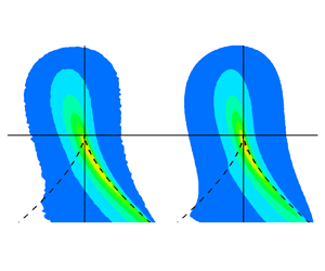
  $Re_\lambda$ (Das & Girimaji Reference Das and Girimaji2020, Reference Das and Girimaji2022). Therefore, the simpler and more accurate data-driven approach of direct tabulation based on DNS data is used in this work, which can be summarised as follows.
(i) The finite space of
$q$, $r$, $a_2$ and ${\tilde {\omega }}_2$, as given in (2.10a,b), is discretised into $(60,60,30,30)$ uniform bins. This discretisation strikes the appropriate balance between sampling accuracy in the bins and the desired details of nonlocal flow physics to be captured. Other discretisations are tested to show convergence to this combination for the most accurate results.(ii) The conditional expectations of the tensors,
$\langle \tilde {h}_{ij} \mid q,r,a_2,{\tilde {\omega }}_2 \rangle$ and $\langle \tilde {\tau }_{ij} \mid q,r,a_2,{\tilde {\omega }}_2 \rangle$, are computed in this discrete phase-space, using DNS data set of forced isotropic turbulence (see Appendix G for details of the data set). Note that lookup tables for only one $Re_\lambda$ is required to model the mean non-local dynamics for turbulent flows of different $Re_\lambda$. Further, this data-driven closure is rotationally invariant since the input and output variables do not depend on the flow reference frame.(iii) This lookup table can then be accessed by an inexpensive array-indexing operation, to determine the conditional mean pressure and viscous dynamics in the principal frame for a given
$(q,r,a_2,{\tilde {\omega }}_2)$ at any point in the flow field or following a fluid particle. This is then transformed into the flow reference frame (3.12) based on the local eigen-directions of strain-rate tensor, to be used in $\mu _{ij}$ for computations.


This completes the modelling of the mean drift tensor  $\mu _{ij}$ as a function of the local
  $b_{ij}$. It is straightforward to show that our data-driven model for
  $\mu _{ij}$ is Galilean invariant (Appendix E).
Our previous work has shown the universality of  $b_{ij}$ statistics and associated nonlocal processes across different types of turbulent flows (Das & Girimaji Reference Das and Girimaji2022). Therefore, here we restrict ourselves to forced isotropic turbulence. We use DNS data of isotropic turbulence at different Reynolds numbers (Appendix G) to illustrate the universality of different modelling components. The
  $b_{ij}$ model closures (lookup tables) developed using the
  $Re_\lambda =427$ data are used at all Reynolds numbers.
3.3.2. Diffusion coefficient tensor
As discussed at the beginning of this section, the interrelationship between the tensors  $D_{ijkl}$ and
  $\gamma _{ij}$ is important in guaranteeing that the mathematical and physical constraints of
  $b_{ij}$ are satisfied. This relationship holds if we use their functional forms, as given in (3.4), in terms of
  $K_{ijkl}$ of the
  $A_{ij}$ SDE. Given the small-scale universality of turbulence at high Reynolds numbers
  $Re_\lambda >200$ (Das & Girimaji Reference Das and Girimaji2019, Reference Das and Girimaji2022), here we model the velocity-gradient dynamics for isotropically forced high-Reynolds-number turbulence. Therefore, we assume a general isotropic form of the fourth-order diffusion coefficient tensor,
  $K_{ijkl}$, of the
  $A_{ij}$ SDE following previous models (Girimaji & Pope Reference Girimaji and Pope1990; Chevillard et al. Reference Chevillard, Meneveau, Biferale and Toschi2008; Johnson & Meneveau Reference Johnson and Meneveau2016a):
 \begin{equation} K_{ijkl} = A^{3/2} ( c_1 \delta_{ij}\delta_{kl} + c_2 \delta_{ik}\delta_{jl} + c_3 \delta_{il}\delta_{jk} ) ,\end{equation}
where  $c_1,c_2,c_3$ are constant dimensionless diffusion coefficients of the model. Only two of these three coefficients are independent subject to the incompressibility condition:
 \begin{equation} \left.\begin{gathered}
K_{iikl} = A^{3/2} ( c_1 \delta_{ii}\delta_{kl} + c_2
\delta_{ik}\delta_{il} + c_3 \delta_{il}\delta_{ik} ) = (3
c_1 + c_2 + c_3) \delta_{kl} = 0 \\ \implies c_1 ={-}
\dfrac{c_2+c_3}{3} \end{gathered}\right\}.
\end{equation}
\begin{equation} \left.\begin{gathered}
K_{iikl} = A^{3/2} ( c_1 \delta_{ii}\delta_{kl} + c_2
\delta_{ik}\delta_{il} + c_3 \delta_{il}\delta_{ik} ) = (3
c_1 + c_2 + c_3) \delta_{kl} = 0 \\ \implies c_1 ={-}
\dfrac{c_2+c_3}{3} \end{gathered}\right\}.
\end{equation}
From (3.4), (3.14) and (3.15), the diffusion coefficient tensor of the  $b_{ij}$ equation is
 \begin{equation} D_{ijkl} = c_2 ( - \tfrac{1}{3}\delta_{ij}\delta_{kl} + \delta_{ik}\delta_{jl} - b_{ij}b_{kl} ) + c_3 ( - \tfrac{1}{3}\delta_{ij}\delta_{kl} + \delta_{il}\delta_{jk} - b_{ij}b_{lk} ),\end{equation}
and
 \begin{equation} \gamma_{ij} ={-} ( \tfrac{7}{2}(c_2^2 + c_3^2) + (2+6q)c_2c_3 ) b_{ij} - 2 c_2 c_3 b_{ji}.\end{equation}
To determine the constant coefficients,  $c_2$ and
  $c_3$, we use a moments constraint method similar to Girimaji & Pope (Reference Girimaji and Pope1990). In this method, the equations of second- and third-order moments of
  $b_{ij}$ are constrained to the values obtained from DNS. First, the SDEs for the second (
 $q$) and third (
 $r$) invariants, as defined in (2.7a,b), are derived from the
  $b_{ij}$-SDE (3.3) using Itô's lemma (A3):
 \begin{equation} \left.\begin{gathered}
{\rm d} q ={-} ( b_{ij} \mu_{ji} + b_{ij}\gamma_{ji} +
\tfrac{1}{2}D_{ijkl}D_{jikl} ) \, {\rm d} t'- b_{ij}
D_{jimn} \, {\rm d} W'_{mn} \\ {\rm d} r ={-} (
b_{ik}b_{kj}\mu_{ji} + b_{ik}b_{kj}\gamma_{ji} + b_{ij}
D_{jkmn} D_{kimn} ) \, {\rm d} t' - b_{ij}b_{jk}D_{kimn} \,
{\rm d} W'_{mn} \end{gathered}\right\}.
\end{equation}
\begin{equation} \left.\begin{gathered}
{\rm d} q ={-} ( b_{ij} \mu_{ji} + b_{ij}\gamma_{ji} +
\tfrac{1}{2}D_{ijkl}D_{jikl} ) \, {\rm d} t'- b_{ij}
D_{jimn} \, {\rm d} W'_{mn} \\ {\rm d} r ={-} (
b_{ik}b_{kj}\mu_{ji} + b_{ik}b_{kj}\gamma_{ji} + b_{ij}
D_{jkmn} D_{kimn} ) \, {\rm d} t' - b_{ij}b_{jk}D_{kimn} \,
{\rm d} W'_{mn} \end{gathered}\right\}.
\end{equation}
Taking the mean of the above equations and substituting the expressions for  $D_{ijkl}$ and
  $\gamma _{ij}$ from (3.16) and (3.17), yields the following differential equations of the moments
  $\langle q \rangle$ and
  $\langle r \rangle$:
 \begin{align} \frac{{\rm d} \langle q \rangle}{ {\rm d} t'} & ={-} \langle b_{ij} \mu_{ji} \rangle - \langle b_{ij}\gamma_{ji} \rangle - \frac{1}{2} \langle D_{ijkl}D_{jikl} \rangle \nonumber\\ & ={-} \langle b_{ij} \mu_{ji} \rangle - ( c_2^2 + c_3^2 )( 8\langle q\rangle + 1 ) - c_2c_3 ( 16 \langle q^2\rangle + 4\langle q\rangle + 4 ), \end{align}
 \begin{align} \frac{{\rm d} \langle r \rangle}{ {\rm d} t'} & ={-} \langle b_{ik}b_{kj}\mu_{ji} \rangle - \langle b_{ik}b_{kj}\gamma_{ji} \rangle - \langle b_{ij} D_{jkmn} D_{kimn} \rangle \nonumber\\ & ={-} \langle b_{ik} b_{kj} \mu_{ji} \rangle - ( c_2^2 + c_3^2 )\left( \frac{27}{2} \langle r \rangle \right) - c_2c_3 ( 6\langle r \rangle + 30 \langle qr \rangle - 6 \langle b_{ij}b_{jk}b_{ik} \rangle ). \end{align}
To model a statistically stationary solution of the VGs, the rate-of-change of moments must be driven to zero while ensuring that the moment values converge to that of DNS. For this, we equate the right-hand side to the negative of the error term:
 $$\begin{gather} \frac{{\rm d} \langle q \rangle}{ {\rm d} t'} ={-} \langle b_{ij} \mu_{ji} \rangle - ( c_2^2 + c_3^2 )( 8\langle q\rangle + 1 ) - c_2c_3 ( 16 \langle q^2\rangle + 4\langle q\rangle + 4 ) ={-} R ( \langle q \rangle - \bar{q} ) , \end{gather}$$
 $$\begin{gather}\frac{{\rm d} \langle r \rangle}{ {\rm d} t'} ={-} \langle b_{ik} b_{kj} \mu_{ji} \rangle - ( c_2^2 + c_3^2 )\left( \frac{27}{2} \langle r \rangle \right) - c_2c_3 ( 6\langle r \rangle + 30 \langle qr \rangle - 6 \langle b_{ij}b_{jk}b_{ik} \rangle) ={-} R (\langle r \rangle - \bar{r} ), \end{gather}$$
where  $\bar {q}, \bar {r}$ are the global mean of
  $q,r$ obtained from DNS data. Here,
  $R$ represents the rate of convergence of these moments and is set to unity. An a priori simulation of the
  $b_{ij}$ model equations is run in the normalised timescale
  $t'$, with an ensemble of 40 000 particles. At each time step, the above system of nonlinear equations is solved using Newton's method to determine the values of the coefficients
  $c_2,c_3$. In this a priori run, as the model's moments,
  $\langle q \rangle$ and
  $\langle r \rangle$, converge very close to the DNS values of
  $\bar {q}$ and
  $\bar {r}$, the coefficients converge to the following values:
 \begin{equation}
c_2=0.009877, \quad c_2 = -0.06402.
\end{equation}
\begin{equation}
c_2=0.009877, \quad c_2 = -0.06402.
\end{equation}
These optimised diffusion coefficient values are used in the stochastic model for  $b_{ij}$ and are insensitive to Reynolds number variation at high enough
  $Re_\lambda$.
3.4. Model for VG magnitude
The Lagrangian evolution of the scalar  $\theta ^*$ (2.12) is modelled using a modified lognormal approach. The magnitude
  $A$ has a nearly lognormal probability distribution and exponential decay of autocorrelation in time (Kolmogorov Reference Kolmogorov1962; Oboukhov Reference Oboukhov1962; Yeung & Pope Reference Yeung and Pope1989). The exponentiated OU process is a statistically stationary process that satisfies both these properties (Uhlenbeck & Ornstein Reference Uhlenbeck and Ornstein1930; Pope & Chen Reference Pope and Chen1990) and is therefore ideal for modelling
  $\theta ^*$. Although it has been pointed out that pseudodissipation rate (
 $\sim A^2$) cannot be precisely lognormal in the context of multifractal formalism (Mandelbrot Reference Mandelbrot1974; Meneveau & Sreenivasan Reference Meneveau and Sreenivasan1991), the OU process models the overall dynamics of
  $A$ quite accurately (Girimaji & Pope Reference Girimaji and Pope1990; Pope & Chen Reference Pope and Chen1990). In fact, a recent analysis of Lagrangian trajectories in high-Reynolds-number turbulence (Huang & Schmitt Reference Huang and Schmitt2014) has shown evidence that the autocorrelation function of
  $A$ is consistent with both the exponential decay prescribed by the OU process as well as the logarithmic decay suggested by the multifractal framework, and the two are nearly indistinguishable at such high Reynolds numbers (Pereira et al. Reference Pereira, Moriconi and Chevillard2018). Since the focus of this work is to accurately reproduce the overall Lagrangian dynamics of the VGs in turbulence, we model the VG magnitude as a Reynolds-number-dependent modified lognormal process, without explicitly accounting for multifractal behaviour.
The OU process is a stationary continuous Gaussian Markov process that is often used in modelling systems of finance, mathematics and physical and biological sciences (Pope & Chen Reference Pope and Chen1990; Klebaner Reference Klebaner2012). It further shows the property of mean reversion. The SDE for a general OU process  $\theta ^*$ evolving in time
  $t^*$ is given by (Girimaji & Pope Reference Girimaji and Pope1990)
 \begin{equation} {\rm d} \theta^* ={-} \alpha (\theta^*-\langle {\theta^*}\rangle) \, {\rm d} t^* + \beta \, {\rm d} W^*,\end{equation}
where  $\alpha, \beta > 0$ are parameters of the model,
  $t^* = \langle A \rangle t$ is the non-dimensional global timescale and
  $\textrm {d} W^*$ is the increment of a Wiener process or a Gaussian random variable with zero mean and variance
  $\textrm {d} t^*$. The parameter
  $\alpha$ represents the rate of mean reversion, and without loss of generality it is set to unity since the model propagates in normalised timescale
  $t^*$. The expected value
  $\langle {\theta ^*} \rangle =0$, by construction, in DNS data. Therefore, the general form of
  $\theta ^*$-SDE used in this work is
 \begin{equation} {\rm d} \theta^* ={-} \theta^* \, {\rm d} t^* + \beta \, {\rm d} W^*.\end{equation}
The diffusion coefficient,  $\beta$, is modelled in three different ways as described in the following subsections.
3.4.1. Model 1: simple OU process
Here, we disregard the dependence of  $\theta ^*$ on
  $b_{ij}$ and consider the simple OU dynamics that satisfies the global mean and global variance of
  $\theta ^*$. In this case, the diffusion coefficient
  $\beta$ is taken to be a constant value, which is calculated as follows. The equation for the global mean is obtained from (3.25),
 \begin{equation} \frac{{\rm d} \langle \theta^* \rangle}{{\rm d} t^*} ={-} \langle \theta^* \rangle . \end{equation}
Thus, the model maintains a stationary mean value of  $\theta ^*$, i.e.
  ${\textrm {d} \langle \theta ^* \rangle }/{\textrm {d} t^*}=0$, once the solution is driven to zero mean (
 $\langle \theta ^* \rangle = 0$) by the mean-reversion property. Next, the equation for the global variance is obtained from (3.25) using Itô's product rule,
 \begin{equation} \frac{{\rm d} \langle {\theta^*}^2 \rangle}{{\rm d} t^*} ={-}2\langle {\theta^*}^2 \rangle + \beta^2. \end{equation}
For a statistically stationary solution, we must have
 \begin{equation} \frac{{\rm d} \langle {\theta^*}^2 \rangle}{{\rm d} t^*} = 0 \quad \implies \quad \beta = \sqrt{2\langle {\theta^*}^2 \rangle}. \end{equation}
Therefore, the final form of the  $\theta ^*$-SDE for Model 1 is given by
 \begin{equation} {\rm d} \theta^* ={-} \theta^* \, {\rm d} t^* + \sqrt{2 \langle {\theta^*}^2 \rangle} \, {\rm d} W^*. \end{equation}
Here, the value of the variance  $\langle {\theta ^*}^2 \rangle = 1$ by definition.
3.4.2. Model 2: modified OU process
Next, we want to ensure that the value of the variance of  $\theta ^*$ conditioned on the local streamline geometry (
 $q,r$) is satisfied. This conditional variance,
  $\langle (\theta ^* - \langle \theta ^* \mid q,r\rangle )^2 \mid q,r \rangle$, is plotted in figure 3 for DNS data of forced isotropic turbulence at different Reynolds numbers. It is evident that the conditional variance of
  $\theta ^*$ shows a clear dependence on
  $q$ and
  $r$, and is nearly invariant with changing
  $Re_\lambda$. Therefore, we modify the diffusion coefficient as
 \begin{equation} \beta = \beta(q,r), \end{equation}
to account for the correct conditional variance of  $\theta ^*$ for a given
  $q$–
$q$– $r$ value. The equation for the conditional variance can be derived from (3.25) as
 \begin{equation} \frac{{\rm d}}{{\rm d} t^*} \langle (\theta^* - \langle \theta^*\mid q,r\rangle)^2 \mid q,r \rangle ={-} 2 \langle {\theta^*}^2 \mid q,r \rangle + \langle {\theta^*} \mid q,r \rangle^2 + (\beta(q,r))^2. \end{equation}
The conditional variance remains stationary only if
 \begin{align} \frac{{\rm d} }{{\rm d} t^*} \langle (\theta^* - \langle \theta^* \mid q,r\rangle)^2 \mid q,r \rangle = 0 \quad \implies \quad \beta(q,r) = \sqrt{2(\langle {\theta^*}^2 \mid q,r \rangle - \langle \theta^* \mid q,r \rangle^2 )}. \end{align}
Therefore, the final SDE of  $\theta ^*$ for Model 2 is given by
 \begin{equation} {\rm d} \theta^* ={-} \theta^* \, {\rm d} t^* + \sqrt{2(\langle {\theta^*}^2 \mid q,r \rangle - \langle \theta^* \mid q,r \rangle^2 )} \, {\rm d} W^*. \end{equation}
Here, the conditional variance values are obtained from DNS data of one  $Re_\lambda$ by discretising the
  $q,r$ space into
  $30\times 30$ bins. The same conditional variance table is applicable when modelling turbulent flows of different Reynolds numbers, as evident from figure 3. This
  $\theta ^*$-model is weakly coupled with the
  $b_{ij}$ dynamics since it depends on
  $q,r$.

Figure 3. Conditional variance of  $\theta ^*$ conditioned on
  $q$–
$q$– $r$, i.e.
  $\langle (\theta ^* - \langle \theta ^* \mid q,r \rangle )^2 \mid q,r \rangle$, for isotropic turbulent flows of Taylor Reynolds numbers: (a)
  $Re_\lambda =225$; (b)
  $Re_\lambda =385$; (c)
  $Re_\lambda =427$; and (d)
  $Re_\lambda =588$.
3.4.3. Model 3: consistent modified OU process
Model 1 ensures that the constant diffusion coefficient captures the accurate global variance of  $\theta ^*$, whereas Model 2 enforces the accurate modelling of conditional variance of
  $\theta ^*$ for a given
  $q,r$. Finally, in Model 3 we propose an adjustment to Model 2 such that both the conditional and global variances are satisfied. For this, we propose to shift the conditional-variance-based diffusion coefficient of Model 2 by a constant value,
  $\beta _0$, as follows:
 \begin{equation} {\rm d} \theta^* ={-} \theta^* \, {\rm d} t^* + ( \sqrt{2(\langle {\theta^*}^2 \mid q,r \rangle - \langle \theta^* \mid q,r \rangle^2 )} + \beta_0 )\, {\rm d} W^*. \end{equation}
Here, the value of  $\beta _0$ is calculated based on the solutions of Models 1 and 2. Model 3 also depends upon
  $b_{ij}$ through its invariants
  $(q,r)$.
3.5. Model summary
The resulting model for the Lagrangian evolution of the complete VG tensor in a turbulent flow is described by a system of SDEs for the normalised VG tensor,  $b_{ij}$, and a separate SDE for the standardised VG magnitude,
  $\theta ^*$.
The final system of equations for evolution of  $b_{ij}$ in local timescale (
 $t'$) is given by
 \begin{gather} {\rm d} b_{ij} = (\mu_{ij} + \gamma_{ij}) \, {\rm d} t' + D_{ijkl} \, {\rm d} W'_{kl}, \end{gather}
 \begin{gather} \mu_{ij} ={-} b_{ik} b_{kj} + \tfrac{1}{3} b_{km}b_{mk} \delta_{ij} + b_{ij} b_{mk} b_{kn} b_{mn} + \langle h_{ij} \mid \boldsymbol{b} \rangle - b_{ij}b_{kl} \langle h_{kl} \mid \boldsymbol{b} \rangle \nonumber\\ + \,\langle \tau_{ij} \mid \boldsymbol{b} \rangle - b_{ij}b_{kl} \langle \tau_{kl} \mid \boldsymbol{b} \rangle , \end{gather}
 $$\begin{gather} \gamma_{ij} ={-} ( \tfrac{7}{2}(c_2^2 + c_3^2) + (2+6q)c_2c_3 ) b_{ij} - 2 c_2 c_3 b_{ji}, \end{gather}$$
 $$\begin{gather}D_{ijkl} = c_2 ( - \tfrac{1}{3}\delta_{ij}\delta_{kl} + \delta_{ik}\delta_{jl} - b_{ij}b_{kl} ) + c_3 ( - \tfrac{1}{3}\delta_{ij}\delta_{kl} + \delta_{il}\delta_{jk} - b_{ij}b_{lk} ). \end{gather}$$
Here, the diffusion coefficient values are
 \begin{equation} c_2 = 0.009877 , \quad c_3 ={-}0.06402. \end{equation}
The conditional mean normalised pressure Hessian and viscous Laplacian tensors are obtained from the data-driven closure in the strain-rate ( $\boldsymbol {s}$) eigen-reference frame as a function of the current (
 $q,r,a_2,{\tilde {\omega }}_2$), followed by a rotation to the flow reference frame using the local eigenvectors of
  $\boldsymbol {s}$:
 \begin{align} \langle {h}_{ij} \mid \boldsymbol{b} \rangle = Q_{ik} \langle \tilde{h}_{kl} \mid q,r,a_2,{\tilde{\omega}}_2 \rangle Q_{jl}\quad \text{and} \quad \langle {\tau}_{ij} \mid \boldsymbol{b} \rangle = Q_{ik} \langle \tilde{\tau}_{kl} \mid q,r,a_2,{\tilde{\omega}}_2 \rangle Q_{jl} . \end{align}
The above coefficient values and the data-driven closure can be applied to model VG dynamics of incompressible turbulent flows irrespective of the Taylor Reynolds number.
The final SDE for  $\theta ^*$ in global timescale (
 $t^* = \langle A \rangle t$) is as follows.
• Model 1:
(3.41)\begin{equation} {\rm d} \theta^* ={-} \theta^* \, {\rm d} t^* + \sqrt{2 \langle {\theta^*}^2 \rangle} \, {\rm d} W^* .\end{equation}• Model 2:
(3.42)\begin{equation} {\rm d} \theta^* ={-} \theta^* \, {\rm d} t^* + \sqrt{2(\langle {\theta^*}^2 \mid q,r \rangle - \langle \theta^* \mid q,r \rangle^2 )} \, {\rm d} W^* . \end{equation}• Model 3:
(3.43)\begin{equation} {\rm d} \theta^* ={-} \theta^* \, {\rm d} t^* + ( \sqrt{2(\langle {\theta^*}^2 \mid q,r \rangle - \langle \theta^* \mid q,r \rangle^2 )} + \beta_0 )\, {\rm d} W^* .\end{equation}


The diffusion coefficients of Models 2 and 3 are obtained from the tabulated conditional variance of  $\theta ^*$ invariant with
  $Re_\lambda$ (figure 3). From data, the shift factor
  $\beta _0$ is found to be about
  $0.1$ independent of the Reynolds number. The VG magnitude and the VG tensor are then given by
 \begin{equation} A = {\rm e}^{\theta^* \sigma_\theta + \langle \theta \rangle} , \quad A_{ij} = A b_{ij}. \end{equation}
The parameters in the above equation are Reynolds number dependent as shown in figure 2. For the case of  $Re_\lambda =427$, the parameter values as determined from the DNS data are
 \begin{equation} \langle \theta \rangle = 2.7493 , \quad \sigma_\theta = 0.589655 , \quad \langle A \rangle = 18.64173 . \end{equation}
One could potentially use scaling laws to determine these parameter values at different Reynolds numbers. However, developing highly accurate scaling laws requires numerous expensive DNS simulations, which is outside the scope of this work. Here, we have directly used the DNS values of these parameters for the different Reynolds number cases considered, except in the  $Re_{\lambda }=1100$ case for which the parameters are determined by extrapolating the approximate scaling laws (figure 2).
To reconcile between the two different timescales,  $t'$ used for
  $b_{ij}$ evolution and
  $t^*$ used for
  $\theta ^*$ evolution, a simple, closed ordinary differential equation,
 \begin{equation} \frac{{\rm d} t^*}{{\rm d} t'} = \frac{\langle A \rangle}{A},\end{equation}
is solved to determine  $t^*$ for a given
  $t'$. No closure is required for this equation. Finally, the Lagrangian evolution of the VG tensor,
  $A_{ij}$, is obtained by multiplying
  $A$ and
  $b_{ij}$ at different global time
  $t^*$. Overall, the VG model presented here consists of three types of data-based components that are listed in table 1. The four-dimensional lookup tables for normalised pressure Hessian and viscous Laplacian tensors and the two-dimensional table for conditional variance of
  $\theta ^*$ can be used in modelling VG dynamics independent of Reynolds numbers; only the three scalar parameters of the model which are statistics of the VG magnitude are Reynolds number dependent and potentially generalisable in the future with accurate universal scaling laws.
Table 1. Components of model based on DNS data.

4. Numerical procedure
The numerical solution of the model equations involves numerically propagating the VG tensor, in terms of the variables  $b_{ij}$ and
  $\theta ^*$, of an ensemble of 40 000 particles. As the initial conditions for the simulations, the particles are picked at random from a randomly generated incompressible isotropic velocity field. The trajectories are advanced for a total time period of approximately
  $1200\tau _\eta$ following these steps at each update.
(i) The
$b_{ij}$ SDEs (3.35) are numerically propagated in the normalised local timescale $t'$, using a second-order weak predictor–corrector scheme (see Appendix F) with a constant time increment $\textrm {d} t'$. At each step, the conditional mean non-local pressure and viscous contributions are calculated based on the current $(q,r,a_2,{\tilde {\omega }}_2)$ values, using the $(60,60,30,30)$ sized lookup tables.(ii) The
$\theta ^*$ SDE ((3.41), (3.42) or (3.43)) is advanced using the second-order weak predictor–corrector numerical scheme (Appendix B) in the global timescale $t^*$, using a first-order approximation of the increment $\textrm {d} t^* = \langle A \rangle \, \textrm {d} t' / A$ for a fixed value of $\textrm {d} t'$.(iii) To reconcile between the timescales, the value of the global timescale
$t^*$ is obtained for every particle at each $t'$ by numerically solving the ordinary differential equation (3.46) using the implicit second-order trapezium rule method.


In this manner, the model simulation propagates all particles at a uniform local time increment of  $\textrm {d} t'=0.01$, but the global timescale
  $t^*$ varies from one particle to the other depending upon its current VG magnitude. A particle with a smaller magnitude requires fewer steps in
  $t'$ to reach a certain
  $t^*$, than a particle with a larger magnitude. The VG magnitude
  $\theta ^*$ evolves in global time
  $t^*$, which approximately scales with Kolmogorov timescale. On the other hand,
  $b_{ij}$ evolves in local timescale
  $t'$ which varies depending on the current local value of
  $A$. Issues may arise when
  $A < \langle A \rangle$, i.e. when
  $b_{ij}$ evolves faster than
  $\theta ^*$, and appropriate measures should be taken to ensure that
  $dt'$ is suitable to propagate the
  $b_{ij}$ equations. However, particles with such low
  $A$ values do not contribute significantly toward the overall VG statistics. Convergence of the model's results for
  $\textrm {d} t'=0.05,0.01$ and
  $0.002$ suggest that
  $\textrm {d} t'=0.01$ is sufficient here for accurate statistical modelling.
The incompressibility and normalisation constraints are automatically upheld by the model, but are only valid up to the order of numerical error. Therefore, to avoid the accretion of numerical errors over large periods of time, hard constraints of  $b_{ii}=0$ and
  $\|\boldsymbol {b}\|_F=1$ are enforced after every update. The computation time is approximately 1.5–2 hours on a single processor for the model's simulations to achieve statistically stationary solutions. The results of the model's simulations for the three different
  $\theta ^*$-models are illustrated in the next section as Model 1 if (3.41) is used, Model 2 if (3.42) is used and Model 3 if (3.43) is used, each along with the
  $b_{ij}$ (3.35). The convergence of all the major results have been tested for these models by performing the simulations with 40 000 and 100 000 particles.
5. Results and comparison with DNS data
This section presents a statistical analysis of the solutions of the three models and a comparison with the statistics of the corresponding DNS data and some previous models. Detailed model results are exhibited for one Reynolds number ( $Re_{\lambda }=427$) and compared with the corresponding DNS data. Specifically, results of VG magnitude are presented in § 5.1, of normalised VG tensor in § 5.2 and of the full VG tensor in § 5.3. Then, to exhibit the broader applicability of the model, the performance is evaluated at other high Reynolds numbers by comparison with the corresponding DNS data in § 5.4. The time evolution of the model's statistics are illustrated as a function of the global normalised time
  $t^*$. The time-converged statistical results are plotted by averaging over multiple time realisations of the model's solution, separated by at least
  $5\tau _\eta$, well after statistical stationarity has been achieved.
5.1. VG magnitude
The time evolution of the mean and standard deviation of  $\theta ^*$ are plotted for all the three
  $\theta ^*$-model equations in figure 4. Note that the time axes are plotted in logscale to display the transients clearly. The numerical simulation starts from an initially random field, which is inconsistent with the DNS values of
  $\langle \theta \rangle$ and
  $\sigma _\theta$, and therefore the initial values of
  $\langle \theta ^* \rangle$ and
  $\sigma _\theta ^*$ are different from zero and unity, respectively. Over time, the model's solution evolves toward the DNS value achieving a statistically stationary state at about
  $t \approx 7 \tau _\eta$ (
 $t^*\approx 6$), where
  $t$ is the real time. As expected, the mean is captured equally well by all three models due to the mean-reversion property of the OU process. The standard deviation is reproduced accurately by both Models 1 and 3 but not as well by Model 2. This indicates that imposing
  $\theta ^*$ to satisfy the variance conditioned on local streamline geometry (
 $q,r$) in Model 2 does not necessarily guarantee that the global variance of
  $\theta ^*$ is automatically satisfied. This justifies the need for the third model to satisfy both the global and conditional standard deviation values.

Figure 4. Evolution of  $\theta ^*$ statistics: (a) mean,
  $\langle \theta ^* \rangle$ and (b) standard deviation,
  $\sigma _{\theta ^*}$, of the three models for
  $Re_{\lambda }=427$. The DNS statistics are marked by dashed lines. The time axis is in logscale.
The converged p.d.f. of the standardised VG magnitude,  $\theta ^*$, for all the models and DNS data are plotted in figure 5. Models 1 and 3 are able to reproduce the
  $\theta ^*$ p.d.f. very well, whereas Model 2 shows deviation from the desired DNS distribution. The plot in the log–linear scale confirms that the converged p.d.f.s of Models 1 and 3 agree well with that of DNS even near the extreme tails of the p.d.f.s. The p.d.f. of VG magnitude (
 $A/\langle A\rangle$: figure 6) is captured equally well by all models near the peak, whereas the high-magnitude tails are reproduced more accurately by Models 1 and 3 compared with Model 2. In fact, a closer inspection suggests that Model 3 provides an improved approximation of the tails over Model 1.

Figure 5. P.d.f. of standardised VG magnitude  $\theta ^*$ in: (a) linear–linear scale and (b) linear–log scale, for
  $Re_{\lambda }=427$. The black solid lines with symbols represent the
  $\theta ^*$-p.d.f. from DNS data.

Figure 6. P.d.f. of VG magnitude,  $A/\langle A\rangle$, for
  $Re_{\lambda }=427$. The black solid line with symbols represents the p.d.f. from DNS data.
5.2. Normalised VG tensor
The conditional mean trajectories (CMTs) in the phase plane of normalised VG invariants  $(q,r)$ are examined as an a priori test of the data-driven closure used to capture the conditional mean non-local effects of pressure and viscosity (§ 3.3.1) on the
  $b_{ij}$-dynamics. The
  $q$–
$q$– $r$ CMTs are obtained by integrating the vector field of conditional mean velocity (
 $\tilde {\boldsymbol {v}}$) in the
  $q$–
$q$– $r$ plane:
 \begin{align} \tilde{\boldsymbol{v}} & = \begin{pmatrix} \tilde{v}_q\\ \tilde{v}_r \end{pmatrix} = \left\langle\left. \begin{pmatrix} {\rm d} q/ {\rm d} t'\\ {\rm d} r/ {\rm d} t' \end{pmatrix} \right| q,r \right\rangle \nonumber\\ & = \left\langle\left. \begin{pmatrix} -3r + 2q b_{ij}b_{ik}b_{kj} - h_{ij} (b_{ji} + 2q b_{ij}) - \tau_{ij} (b_{ji} + 2q b_{ij}) \\ \tfrac{2}{3}q^2 + 3rb_{ij}b_{ik}b_{kj} - h_{ij}(b_{jk}b_{ki} + 3rb_{ij}) - \tau_{ij}(b_{jk}b_{ki} + 3rb_{ij}) \end{pmatrix} \right| q,r \right\rangle , \end{align}
due to the inertial, pressure and viscous processes in the turbulent flow. Note that the effect of the large-scale forcing is not included here because it is not accounted for in the data-driven closure but rather in the stochastic forcing (diffusion) term in the  $b_{ij}$-SDE, which cannot be tested a priori. The
  $q$–
$q$– $r$ CMTs obtained directly from DNS data are plotted in figure 7(a). As discussed in Das & Girimaji (Reference Das and Girimaji2022), trajectories closer to the origin converge towards the attractor near the origin (represents pure-shear streamlines) whereas trajectories that are outside the separatrix loop are attracted towards the bottom line attractor (represents pure-strain streamlines). This behaviour is almost exactly replicated in the
  $q$–
$q$– $r$ CMTs computed using the model's data-driven closure for the conditional mean pressure Hessian and viscous Laplacian tensors (figure 7b). The close resemblance between the two is somewhat expected given the very nature of the lookup table approach for closure.

Figure 7. CMTs in the  $q$–
$q$– $r$ plane due to the inertial, pressure and viscous effects obtained using (a) DNS data and (b)
  $b_{ij}$ data-driven model. Background contours represent the speed of the trajectory at each point, given by the magnitude of the conditional mean velocity vector,
  $|\tilde {\boldsymbol {v}}|$.
Now, we compare the a posteriori results of the normalised VG tensor of the model with that of DNS. First, we study the moments of the second ( $q$) and third (
 $r$) invariants of the tensor, which are important quantities that determine the geometric shape of the local flow streamlines. The evolution of up to fourth-order moments of
  $q$ and
  $r$ are plotted for each model in figure 8. It is first evident that the three models with the same
  $b_{ij}$-SDE but different
  $\theta ^*$-SDEs produce nearly identical
  $q,r$ moments. Thus, it appears that the variation in the
  $\theta ^*$ model does not have a discernible impact on the
  $b_{ij}$ statistics of the models. Starting from a randomly generated set of initial conditions, the
  $b_{ij}$-SDE drives the solution towards convergence to a statistically stationary state at
  $t \approx 72 \tau _\eta$ (
 $t^* \approx 60$). Therefore, to converge in
  $b_{ij}$ statistics, our model takes approximately
  $10$ times as long as it takes to reach statistical stationarity in
  $\theta ^*$. Up to at least fourth-order moments of
  $q$ and
  $r$ produced by the model are reasonably close to the DNS values. Further, the time evolution of moments of correlation between
  $q$ and
  $r$, i.e.
  $\langle qr \rangle$, and
  $\langle q^2 r^2 \rangle$, are plotted in figure 9. These moments show a slightly larger deviation from the DNS values as compared with all other moments.

Figure 8. Evolution of  $q$ and
  $r$ statistics in global normalised time
  $t^*$. Means: (a)
  $\langle q \rangle$ and (b)
  $\langle r \rangle$. Second-order moments: (c)
  $\langle q^2 \rangle$ and (d)
  $\langle r^2 \rangle$. Third-order moments: (e)
  $\langle q^3 \rangle$ and ( f)
  $\langle r^3 \rangle$. Fourth-order moments: (g)
  $\langle q^4 \rangle$ and (h)
  $\langle r^4 \rangle$ for the three models. The dashed lines represent the DNS statistics. The time axis is in log-scale.

Figure 9. Evolution of the  $q$ and
  $r$ moments, (a)
  $\langle qr \rangle$, and (b)
  $\langle q^2 r^2 \rangle$, in global normalised time
  $t^*$. The dashed lines represent the DNS statistics. The time axis is in log-scale.
The evolution of  $q$–
$q$– $r$ joint p.d.f. is plotted at different times (
 $t^*$) with ensembles of only
  $40\ 000$ particles propagated by Model 3 in figure 10. The solutions of the other two models show similar trends and are, therefore, not presented separately. The joint p.d.f. of the initial field (
 $t^*=0$) is symmetric in
  $r$, as expected from a joint Gaussian distribution. As time progresses, the modelled dynamics cause the p.d.f. to skew towards the right zero-discriminant line. The p.d.f. contours shrink in size and steepen in magnitude as more and more particles accumulate along the right zero-discriminant line. This finally results in the characteristic teardrop-like shape, which becomes nearly invariant beyond
  $t^* \approx 60$. In this manner, our model reproduces the teardrop-shaped
  $q$–
$q$– $r$ joint p.d.f., one of the key signatures of small-scale turbulence (Soria et al. Reference Soria, Sondergaard, Cantwell, Chong and Perry1994; Chong et al. Reference Chong, Soria, Perry, Chacin, Cantwell and Na1998; Wallace Reference Wallace2009; Das & Girimaji Reference Das and Girimaji2020).

Figure 10. Evolution of the  $q$–
$q$– $r$ joint p.d.f. during numerical propagation of Model 3 at different global normalised time: (a)
  $t^* = 0.0$, (b)
  $t^* = 0.1$, (c)
  $t^* = 0.3$, (d)
  $t^* = 1.0$, (e)
  $t^* = 2.0$, ( f)
  $t^* = 5.0$, (g)
  $t^* = 10.0$, (h)
  $t^* = 50.0$ and (i)
  $t^* = 500.0$. The dashed lines represent the lines of zero discriminant
  $(d = q^3 + (27/4)r^2) = 0$.
The converged  $q$–
$q$– $r$ joint p.d.f., averaged over multiple time realisations in the stationary state of the models’ solutions, are plotted in figure 11(a–c) for the three models. It is clear that all three models produce nearly identical
  $q$–
$q$– $r$ joint p.d.f.s showing excellent resemblance to that obtained from DNS data (figure 11d). An extremely close comparison shows that the model results in slightly thinner p.d.f. contours in the strain-dominated bottom half of the teardrop and is slightly wider in the rotation-dominated top half than DNS. Overall, the model is able to reproduce the joint p.d.f. of
  $q$–
$q$– $r$, one of the key features of VG geometry in turbulence with reasonable accuracy and without any discernible distortion such as those commonly observed in previously proposed VG models (Johnson & Meneveau Reference Johnson and Meneveau2016a; Pereira, Garban & Chevillard Reference Pereira, Garban and Chevillard2016).

Figure 11. Joint p.d.f.s of  $q$–
$q$– $r$ obtained from the solutions of (a) Model 1, (b) Model 2, (c) Model 3 and (d) DNS data at
  $Re_{\lambda }=427$. The dashed lines represent the zero-discriminant lines.
The alignment of vorticity with strain-rate eigen-directions is another key feature of small-scale turbulence (Tsinober Reference Tsinober2009; Wallace Reference Wallace2009). From (2.6) in the eigen-reference frame of the strain-rate tensor, one can show that the cosine of the angles of alignment between the vorticity vector and the three strain-rate eigenvectors are given by
 \begin{equation} \cos{\phi_i} = \frac{{\tilde{\omega}}_i}{|\boldsymbol{{\tilde{\omega}}}|} \quad {\text{for }} i = 1,2,3. \end{equation}
The angles  $\phi _1$,
  $\phi _2$ and
  $\phi _3$ represent the angles of alignment of vorticity with the most expansive, intermediate and most compressive strain-rate eigenvectors, respectively. In figure 12, the converged p.d.f.s of the absolute values of the cosine of alignment angles are plotted for Model 3 in comparison with that of DNS. Similar to other
  $b_{ij}$ statistics, the alignment p.d.f.s produced by the other two models are nearly identical to that of Model 3 and are therefore not displayed separately. It is evident that the model is able to capture these p.d.f.s with reasonable accuracy. It reproduces the preferential alignment of vorticity with the intermediate strain-rate eigen-direction (Ashurst et al. Reference Ashurst, Kerstein, Kerr and Gibson1987; Lüthi, Tsinober & Kinzelbach Reference Lüthi, Tsinober and Kinzelbach2005; Buaria, Bodenschatz & Pumir Reference Buaria, Bodenschatz and Pumir2020) reasonably well. It slightly over-predicts the tendency of the vorticity vector to be perpendicular to the compressive strain-rate eigenvector. The alignment with the most expansive strain-rate eigenvector is also captured well by the model.

Figure 12. P.d.f.s of absolute values of cosine of angles between vorticity vector and strain-rate eigenvectors (1, most expansive; 2, intermediate; 3, most compressive). The solid lines are the p.d.f.s obtained from DNS data at  $Re_{\lambda }=427$.
So far, we have established that in terms of the  $\theta ^*$ statistics, Model 3 performs the best showing a slight advantage over Model 1, whereas Model 2 shows the highest deviation from the DNS statistics. Further, the
  $b_{ij}$ model performs remarkably well in reproducing the
  $b_{ij}$ statistics accurately, which does not vary with the
  $\theta ^*$ model. This is somewhat surprising since even though the
  $b_{ij}$-SDE in local time
  $t'$ does not have an explicit dependence on
  $\theta ^*$, the real-time evolution of
  $b_{ij}$ indirectly depends on the local VG magnitude
  $A$ (
$A$ ( ${\sim }e^{\theta ^*}$). Yet, the
  $b_{ij}$ statistics of the model appear to be unchanged with the variation of the
  $\theta ^*$ model equation.
5.3. Full VG tensor
After examining the statistical results of  $b_{ij}$ and
  $A$ individually, we now test the models’ performance in capturing the overall VG (
 $A_{ij}$) statistics. First, the p.d.f.s of the longitudinal (
 $A_{11}$) and transverse (
 $A_{12}$) VGs, normalised by their global root-mean-square values, are examined for all the three models in figure 13. For comparison, we have also plotted the corresponding p.d.f.s obtained from the DNS data and two of the recent VG models that have shown improved results compared with the other models in the literature: (i) recent deformation of Gaussian fields (RDGF) model by Johnson & Meneveau (Reference Johnson and Meneveau2016a) and (ii) physics-informed machine learning (PIML) model by Tian et al. (Reference Tian, Livescu and Chertkov2021). Our models are able to reproduce the skewed
  $A_{11}$-p.d.f. and the symmetric
  $A_{12}$-p.d.f., as observed in DNS, with reasonable accuracy. They show significant improvement in capturing both
  $A_{11}$ and
  $A_{12}$ p.d.f.s compared with the RDGF and PIML models. On closer observation, it is evident that whereas the p.d.f.s are captured nearly perfectly in the densely populated part by all three of our models, there are smaller differences near the tails. Models 1 and 3 predict a slightly heavier-tailed distribution of
  $A_{11}$ than DNS, whereas Model 2 produces a more accurate
  $A_{11}$-p.d.f. On the other hand, Model 3 appears to capture the
  $A_{12}$-p.d.f. tails slightly more accurately than the others.

Figure 13. P.d.f.s of: (a) longitudinal component of VG tensor,  $A_{11}/\sqrt {\langle A^2_{11} \rangle }$, and (b) transverse component of VG tensor,
  $A_{12}/\sqrt {\langle A^2_{12} \rangle }$, in log–linear scale obtained from the solutions of the three models for
  $Re_{\lambda }=427$. The solid line marked with symbols represent the p.d.f.s obtained from DNS data. The dashed and dash-dotted lines represent the p.d.f.s obtained from previous models RDGF (Johnson & Meneveau Reference Johnson and Meneveau2016a) and PIML (Tian et al. Reference Tian, Livescu and Chertkov2021), respectively.
In order to determine the finer differences in the p.d.f.s, we examine the higher-order moments of the VG magnitude,  $A$, as well as VG components,
  $A_{11}$ and
  $A_{12}$. These moment values are compared with that of DNS data and RDGF model of Johnson & Meneveau (Reference Johnson and Meneveau2016a) in table 2. For each moment, the model-produced value closest to DNS is marked in bold. It is evident that the moments of magnitude
  $A$ are best captured by Model 3. The skewness, kurtosis and sixth-order moment of the longitudinal component
  $A_{11}$ are reproduced best in Model 2, although Model 3 is not far behind and is better than Model 1. The skewness of the transverse component
  $A_{12}$ is correctly captured as zero by all the models, maintaining a symmetric probability distribution in each case. The kurtosis and sixth-order moment of
  $A_{12}$ are also captured most closely by Model 3. Overall, Model 3 provides the most accurate representation of the probability distributions and moments of the VG tensor. It is important to note that the values of the higher-order velocity-gradient moments of the DNS data at the resolution (
 $k_{max} \eta \approx 1.4$) used in the present study and in that of Johnson & Meneveau (Reference Johnson and Meneveau2016a), may change with increasing resolution, as suggested by recent works (Yeung et al. Reference Yeung, Sreenivasan and Pope2018; Buaria et al. Reference Buaria, Pumir, Bodenschatz and Yeung2019; Buaria & Pumir Reference Buaria and Pumir2022). It is reasonable to expect that the proposed model will capture the appropriate values if trained on the higher-resolution data sets.
Table 2. Third-, fourth- and sixth-order moments of VG magnitude ( $A=\sqrt {A_{ij}A_{ij}}$), longitudinal VG component (
 $A_{11}$), transverse VG component (
 $A_{12}$) from DNS data, Model 1, Model 2, Model 3 and RDGF model of Johnson & Meneveau (Reference Johnson and Meneveau2016a) for
  $Re_{\lambda }=427$. For each moment, the DNS value and the model's value closest to DNS are written in bold.

The p.d.f.s of dissipation rate ( $\nu S_{ij}S_{ij}$), enstrophy (
 $\nu W_{ij}W_{ij}$), and pseudodissipation rate (
 $\nu A_{ij}A_{ij}$), normalised by their global means, computed from the converged stationary state solutions of all three models are plotted in figure 14. The p.d.f.s obtained from DNS data and those available from the RDGF model (Johnson & Meneveau Reference Johnson and Meneveau2016a) are also illustrated for comparison, along with the p.d.f.s for the initial Gaussian field used in our model's simulations. It is interesting to note that starting from this Gaussian field, the model develops a turbulent flow field solution closely resembling that of DNS with the characteristic p.d.f. tails at extreme values. It is clear that all three models reproduce the heavy-tailed probability distributions of both dissipation and enstrophy more accurately than the RDGF model. Model 2 provides the most accurate representation of the dissipation p.d.f. whereas Models 1 and 3 over-predict the probability of occurrence of large dissipation rates near the tails of the p.d.f. Enstrophy, which is more intermittent in nature than dissipation rate (Meneveau et al. Reference Meneveau, Sreenivasan, Kailasnath and Fan1990; He et al. Reference He, Chen, Kraichnan, Zhang and Zhou1998; Zeff et al. Reference Zeff, Lanterman, McAllister, Roy, Kostelich and Lathrop2003; Yeung et al. Reference Yeung, Sreenivasan and Pope2018; Buaria et al. Reference Buaria, Pumir, Bodenschatz and Yeung2019; Buaria & Pumir Reference Buaria and Pumir2022), is captured best by Model 3. Models 1 and 2, on the other hand, under-predict the probability density of enstrophy near the tails. Taking the sum of the dissipation rate and enstrophy results in the pseudodissipation rate, which is reproduced quite accurately by Model 3, even near the extreme tails. Overall, the results of Model 3 constitute the closest representation of the VG statistics in turbulent flows.

Figure 14. P.d.f.s of: (a) dissipation rate,  $S_{ij}S_{ij}/{\langle S_{ij}S_{ij} \rangle }$, (b) enstrophy,
  $W_{ij}W_{ij}/{\langle W_{ij}W_{ij} \rangle }$, and (c) pseudodissipation rate,
  $A_{ij}A_{ij}/{\langle A_{ij}A_{ij} \rangle }$, obtained from the three models for
  $Re_{\lambda }=427$. Black solid lines with symbols represent the p.d.f.s obtained from DNS data; black dash-dotted lines mark the p.d.f.s for the initial field used in the model's simulations; magenta dashed lines represent the p.d.f.s from the RDGF model of Johnson & Meneveau (Reference Johnson and Meneveau2016a).
5.4. Reynolds number dependence
Finally, we examine the model performance at different Reynolds numbers. The normalised VG behaviour is nearly independent of Reynolds number above a certain  $Re_{\lambda }$ as shown in our previous studies (Das & Girimaji Reference Das and Girimaji2019, Reference Das and Girimaji2022). Therefore, we only examine the p.d.f.s of pseudodissipation rate and invariants
  $(Q,R)$ of the VG tensor.
Figure 15 shows the p.d.f.s of pseudodissipation rate ( $A^2 = A_{ij}A_{ij}$) obtained at different
  $Re_{\lambda }$ using Model 3. It is evident that the model captures the expected trend of increasing probability of high pseudodissipation rate values with increasing Reynolds number. In addition, the p.d.f.s of the model's pseudodissipation rate at each of these Reynolds numbers also compare reasonably well with that of the corresponding DNS data, as shown in figure 16. The model reproduces the p.d.f. accurately up to a large extent at the tails. It is evident that the model generalises reasonably well to higher Reynolds numbers.

Figure 15. P.d.f. of pseudodissipation rate,  $A_{ij}A_{ij}/\langle A_{mn} A_{mn} \rangle$, obtained from different Reynolds number solutions of Model 3. Reynolds numbers illustrated:
  $Re_{\lambda } = \{225,385,427,588,{1100}\}$.

Figure 16. P.d.f. of pseudodissipation rate,  $A_{ij}A_{ij}/{\langle A_{ij}A_{ij} \rangle }$ for different Reynolds number cases using Model 3: (a)
  $Re_{\lambda }=225$, (b)
  $Re_{\lambda }=385$, (c)
  $Re_{\lambda }=427$, (d)
  $Re_{\lambda }=588$ and (e)
  $Re_{\lambda }=1100$. Black solid lines with squares represent p.d.f.s from DNS data. P.d.f. for
  $Re_{\lambda }=1100$ case is obtained from Elsinga, Ishihara & Hunt (Reference Elsinga, Ishihara and Hunt2023).
Model predictions also capture the monotonic increase of the VG moments with  $Re_{\lambda }$, as indicated by table 3. Comparison with the corresponding moments from DNS data (when available) shows that Model 3 is able to reproduce the moments of VG magnitude as well as longitudinal/transverse VG components at different Reynolds numbers reasonably well. The error in model prediction is more in higher-order moments (flatness) as expected. The use of more advanced multifractal models for VG magnitude in place of the modified lognormal model will likely improve these statistics.
Table 3. Moments of VGs for different Reynolds numbers. Variance and flatness of VG magnitude ( $A=\sqrt {A_{ij}A_{ij}}$), skewness and flatness of longitudinal
  $A_{11}$, and flatness of transverse
  $A_{12}$ from DNS data and Model 3. Skewness of
  $A_{12}$ is correctly predicted as zero by the model for all cases.

The joint p.d.f.s of the second and third invariants ( $Q,R$) of the VG tensor (
 $A_{ij}$), averaged over multiple time realisations, are plotted in figure 17(a,c) for
  $Re_{\lambda }=427$ and
  $588$, respectively. For comparison, the corresponding
  $Q$–
$Q$– $R$ joint p.d.f.s from DNS data are illustrated in figure 17(b,d). It is evident that the model is able to capture the characteristic teardrop shape of the p.d.f. with a high density of points along the right discriminant line (Soria et al. Reference Soria, Sondergaard, Cantwell, Chong and Perry1994; Chong et al. Reference Chong, Soria, Perry, Chacin, Cantwell and Na1998; Ooi et al. Reference Ooi, Martin, Soria and Chong1999; Wallace Reference Wallace2009). The present model shows improvement over the RDGF (Johnson & Meneveau Reference Johnson and Meneveau2016a) and PIML (Tian et al. Reference Tian, Livescu and Chertkov2021) models in capturing the features of the
  $Q$–
$Q$– $R$ p.d.f. However, a close comparison with DNS shows slight differences in the shapes of the outer low-probability contours of
  $Q$–
$Q$– $R$ joint p.d.f., unlike the near-perfect match achieved in the case of the normalised
  $q$–
$q$– $r$ joint p.d.f. (figure 11). Extending this method to satisfy higher-order conditional moments of VG magnitude will likely improve the results.

Figure 17. Joint p.d.f. of  $Q$–
$Q$– $R$ normalised by the mean VG magnitude
  $(\langle A_{ij} A_{ij} \rangle )$: for
  $Re_{\lambda }=427$ (a) Model 3 and (b) DNS data, and for
  $Re_{\lambda }=588$ (c) Model 3 and (d) DNS data. The dashed lines represent zero-discriminant lines.
6. Conclusion
A stochastic model for the Lagrangian evolution of VG tensor in an incompressible turbulent flow has been presented. The bounded and well-behaved dynamics of the normalised VG tensor ( $b_{ij}$) has been modelled separately from the intermittent VG magnitude (
 $A$). The main non-local flow physics of pressure and viscous processes are easily amenable to generalisation in the compact and bounded framework of
  $b_{ij}$. The closure modelling of important nonlocal effects has been performed using a simple but effective lookup table approach within the four-dimensional compact state space of
  $b_{ij}$. On the other hand, the intermittent magnitude of the VG tensor has been modelled as a modified OU process. The Reynolds-number-dependent conditional variance of the magnitude has been incorporated into the model to better capture intermittency effects.
Numerical simulation of the Lagrangian model takes an initially random field and drives it towards a statistically stationary solution closely resembling DNS small-scale behaviour. The model performs quite well in capturing the Eulerian p.d.f.s and higher-order moments of  $b_{ij}$. Further, it is able to reproduce the characteristic teardrop shape of the joint probability distribution of the
  $b_{ij}$ invariants (
 $q,r$) without any discernible distortion observed in many previous models. The vorticity–strain-rate alignment angles are also captured with reasonable accuracy. The model also reproduces up to sixth-order moments of VGs and the heavy-tailed p.d.f.s of VG magnitude, enstrophy and dissipation rate. Overall, the present model not only reproduces the small-scale geometric features of turbulence but also captures the intermittent nature of magnitude better than the previous models. Most importantly, the model is generalisable to different Reynolds number turbulent flows, facilitated by the modelling of the bounded and nearly universal VG shape separately from the Reynolds-number-dependent VG magnitude. In future work, the magnitude will be modelled as a multifractal process to fully capture the extreme tails of the p.d.f.s and the higher-order moments with even greater accuracy.
Acknowledgements
The authors would like to acknowledge Dr D. Donzis of Texas A&M University for providing part of the DNS data used in this work. The authors would also like to acknowledge Texas A&M High Performance Research Computing, whose resources were used in this work. Part of this work was presented at the American Physical Society (APS) Division of Fluid Dynamics meeting of 2020 and was a part of the PhD dissertation of R.D. at Texas A&M University published in December 2021.
Declaration of interest
The authors report no conflict of interest.
Appendix A. Relevant properties of Itô process
A.1. Itô's lemma for scalar variables
For a SDE of a scalar ( $x$) of the form
 \begin{equation} {{\rm d}\kern0.7pt x} = f(x) \, {\rm d} t + g(x) \, {\rm d} W, \end{equation}
the SDE for a function of the variable,  $\varphi = \varphi ({x})$, is given by
 \begin{equation} {\rm d} (\varphi(x)) = \left( \frac{\partial \varphi}{\partial t} + f(x) \frac{\partial \varphi}{\partial x} + \frac{1}{2}g^2(x) \frac{\partial^2 \varphi}{\partial x^2} \right) \, {\rm d} t + g(x) \frac{\partial \varphi}{\partial x}\, {\rm d} W. \end{equation}
A.2. Itô's lemma for tensorial variables
For a system of SDEs of a tensor,  $X_{ij}$, of the form
 \begin{equation} {\rm d} X_{ij} = F_{ij} (\boldsymbol{X}) \, {\rm d} t + G_{ijkl} (\boldsymbol{X}) \, {\rm d} W_{kl},\end{equation}
the SDE for a function of the tensor,  $\phi = \phi (\boldsymbol {X})$, is given by
 \begin{equation} {\rm d} \phi = \left( \frac{\partial \phi}{\partial t} + F_{ij} \frac{\partial \phi}{\partial X_{ij}} + \frac{1}{2} G_{ijkl} G_{pqkl} \frac{\partial^2 \phi}{\partial X_{ij}X_{pq}} \right) \, {\rm d} t + G_{ijkl} \frac{\partial \phi}{\partial X_{ij}}\, {\rm d} W_{kl}. \end{equation}
A.3. Itô's product rule
For SDEs of two scalar variables,  $x_1$ and
  $x_2$, given by
 $$\begin{gather} {\rm d}\kern0.7pt x_1 = f_1(x_1) \, {\rm d} t + g_1(x_1) \, {\rm d} W , \end{gather}$$
 $$\begin{gather}{\rm d}\kern0.7pt x_2 = f_2(x_2) \, {\rm d} t + g_2(x_2) \, {\rm d} W, \end{gather}$$
the SDE of the product of the two variables is
 \begin{equation} {\rm d} (x_1 x_2) = x_1 \, {\rm d} (x_2) + \, {\rm d} (x_1) x_2 + \, {\rm d} (x_1) \, {\rm d} (x_2). \end{equation}
Appendix B. Derivation of $b_{ij}$ SDE from $A_{ij}$ SDE


The system of SDEs for the VG tensor  $A_{ij}$ is given by
 \begin{equation} \left.\begin{gathered}
d A_{ij} = M_{ij} \, {\rm d} t + K_{ijkl}\, {\rm d} W_{kl}
\\ \text{where, } \langle {\rm d} W_{ij} \rangle = 0 \quad
\text{and} \quad \langle {\rm d} W_{ij}\, {\rm d} W_{kl}
\rangle = \delta_{ik} \delta_{jl} \, {\rm d} t
\end{gathered}\right\}. \end{equation}
\begin{equation} \left.\begin{gathered}
d A_{ij} = M_{ij} \, {\rm d} t + K_{ijkl}\, {\rm d} W_{kl}
\\ \text{where, } \langle {\rm d} W_{ij} \rangle = 0 \quad
\text{and} \quad \langle {\rm d} W_{ij}\, {\rm d} W_{kl}
\rangle = \delta_{ik} \delta_{jl} \, {\rm d} t
\end{gathered}\right\}. \end{equation}
Applying Itô's lemma we can obtain the SDE of the Frobenius norm of the tensor,  $\phi = A^2 = A_{ij}A_{ij}$, as
 \begin{equation} {\rm d}(\phi) = (2A_{ij}M_{ij} + K_{ijkl}K_{ijkl}) \, {\rm d} t + 2 A_{ij} K_{ijkl}\, {\rm d} W_{kl}, \end{equation}
neglecting terms of the order of  $\mathcal {O}(\textrm {d} t^n) \ \forall \, n>1$. Then, the SDE of the VG magnitude,
  $A = \sqrt {A^2} = \sqrt {\phi }$, is obtained using Itô's lemma:
 \begin{equation} {\rm d} (A) = \left( \frac{A_{ij}M_{ij}}{A} + \frac{K_{ijkl}K_{ijkl}}{2A} - \frac{A_{ij}K_{ijkl}A_{mn}K_{mnkl}}{2A^3} \right) {\rm d} t + \frac{A_{ij}K_{ijkl}}{A}\, {\rm d} W_{kl}. \end{equation}
Next, the SDE of its reciprocal s obtained using Itô's lemma
 \begin{equation} {\rm d} \left(\frac{1}{A}\right) ={-} \frac{1}{A^2} \left[ \left( \frac{A_{ij}M_{ij}}{A} + \frac{K_{ijkl}K_{ijkl}}{2A} - \frac{3}{2}\frac{A_{ij}K_{ijkl}A_{mn}K_{mnkl}}{A^3} \right) \, {\rm d} t + \frac{A_{ij}K_{ijkl}}{A}\, {\rm d} W_{kl} \right].\end{equation}
Finally, applying Itô's product rule to determine the SDE for the normalised VG tensor,  $b_{ij} \equiv {A_{ij}}/{A}$,
 \begin{equation} {\rm d} b_{ij} = {\rm d} \left(\frac{1}{A} A_{ij} \right) = \frac{1}{A} \, {\rm d} A_{ij} + A_{ij} \, {\rm d} \left(\frac{1}{A}\right) + {\rm d} A_{ij}\, {\rm d} \left( \frac{1}{A} \right),\end{equation}
and using (B1) and (B4), we obtain
 \begin{align} {\rm d} b_{ij} &= \left( \frac{M_{ij}}{A} - \frac{b_{ij}b_{kl}M_{kl}}{A} -\frac{b_{ij}K_{pqkl}K_{pqkl}}{2A^{2}} - \frac{b_{pq}K_{pqkl}K_{ijkl}}{A^{2}} \right. \nonumber\\ &\quad +\left. \frac{3}{2} \frac{b_{ij}b_{pq}K_{pqkl}b_{mn}K_{mnkl}}{A^{2}} \right) \, {\rm d} t + \left( \frac{K_{ijkl}}{A} - \frac{b_{ij}b_{pq}K_{pqkl}}{A} \right) \, {\rm d} W_{kl}. \end{align}
Rearranging, we can write the final form of the  $b_{ij}$-SDE as follows
 \begin{align} {\rm d} b_{ij} &= \left( \frac{M_{ij}}{A^2} - b_{ij}b_{kl}\frac{M_{kl}}{A^2} -\frac{1}{2}b_{ij}\frac{K_{pqkl}}{A^{3/2}}\frac{K_{pqkl}}{A^{3/2}} - b_{pq}\frac{K_{pqkl}}{A^{3/2}}\frac{K_{ijkl}}{A^{3/2}} \right. \nonumber\\ &\quad + \left.\frac{3}{2} b_{ij}b_{pq}\frac{K_{pqkl}}{A^{3/2}}b_{mn}\frac{K_{mnkl}}{A^{3/2}} \right) {\rm d} t' + \left( \frac{K_{ijkl}}{A^{3/2}} - b_{ij}b_{pq}\frac{K_{pqkl}}{A^{3/2}} \right) {\rm d} W'_{kl}, \end{align}
where  $\textrm {d} t' = A\, \textrm {d} t$ and
  $\textrm {d} W'_{ij} = A^{1/2} \,\textrm {d} W_{ij}$. Note that all the terms on the right-hand side of the
  $b_{ij}$ SDE are non-dimensional, including
  $\textrm {d} t'$,
  $\textrm {d} W'_{kl}$,
  $M_{ij}/A^2$ and
  $K_{ijkl}/A^{3/2}$. This equation can also be written as
 \begin{equation} \left.\begin{gathered}
d b_{ij} = (\mu_{ij} + \gamma_{ij}) \, {\rm d} t' +
D_{ijkl} \, {\rm d} W'_{kl} \quad \text{where}\\
\displaystyle \mu_{ij} = \dfrac{M_{ij}}{A^2} -
b_{ij}b_{kl}\dfrac{M_{kl}}{A^2} , \quad D_{ijkl} =
\dfrac{K_{ijkl}}{A^{3/2}} -
b_{ij}b_{pq}\dfrac{K_{pqkl}}{A^{3/2}} , \\ \displaystyle
\gamma_{ij}
={-}\dfrac{1}{2}b_{ij}\dfrac{K_{pqkl}}{A^{3/2}}\dfrac{K_{pqkl}}{A^{3/2}}
-b_{pq}\dfrac{K_{pqkl}}{A^{3/2}}\dfrac{K_{ijkl}}{A^{3/2}}
+\dfrac{3}{2}b_{ij}b_{pq}\dfrac{K_{pqkl}}{A^{3/2}}b_{mn}\dfrac{K_{mnkl}}{A^{3/2}},
\end{gathered}\right\} \end{equation}
\begin{equation} \left.\begin{gathered}
d b_{ij} = (\mu_{ij} + \gamma_{ij}) \, {\rm d} t' +
D_{ijkl} \, {\rm d} W'_{kl} \quad \text{where}\\
\displaystyle \mu_{ij} = \dfrac{M_{ij}}{A^2} -
b_{ij}b_{kl}\dfrac{M_{kl}}{A^2} , \quad D_{ijkl} =
\dfrac{K_{ijkl}}{A^{3/2}} -
b_{ij}b_{pq}\dfrac{K_{pqkl}}{A^{3/2}} , \\ \displaystyle
\gamma_{ij}
={-}\dfrac{1}{2}b_{ij}\dfrac{K_{pqkl}}{A^{3/2}}\dfrac{K_{pqkl}}{A^{3/2}}
-b_{pq}\dfrac{K_{pqkl}}{A^{3/2}}\dfrac{K_{ijkl}}{A^{3/2}}
+\dfrac{3}{2}b_{ij}b_{pq}\dfrac{K_{pqkl}}{A^{3/2}}b_{mn}\dfrac{K_{mnkl}}{A^{3/2}},
\end{gathered}\right\} \end{equation}
where  $\mu _{ij}$ is the mean drift coefficient tensory,
  $\gamma _{ij}$ is the additional drift coefficient tensor and
  $D_{ijkl}$ is the diffusion coefficient tensor.
Appendix C. Incompressibility constraint
To prove that the system of SDEs of  $b_{ij}$ in (3.4) satisfies the incompressibility constraint, we take the trace on both sides of the
  $b_{ij}$-SDE:
 \begin{equation} {\rm d} b_{ii} = (\mu_{ii} + \gamma_{ii}) \, {\rm d} t' + D_{iikl} \, {\rm d} W'_{kl}.\end{equation}
Now, since  $b_{ii} = 0$ and
  $M_{ii} = 0$ by construction, we have
 \begin{equation} \mu_{ii} = \frac{M_{ii}}{A^2} - b_{ii}b_{kl}\frac{M_{kl}}{A^2} = 0.\end{equation}
Further, since  $K_{iikl} = 0$ by construction, it can be easily shown that
 \begin{equation} \left.\begin{gathered}
\displaystyle \gamma_{ii}
={-}\dfrac{1}{2}b_{ii}\dfrac{K_{pqkl}}{A^{3/2}}\dfrac{K_{pqkl}}{A^{3/2}}
- b_{pq}\dfrac{K_{pqkl}}{A^{3/2}}\dfrac{K_{iikl}}{A^{3/2}}
+
\dfrac{3}{2}b_{ii}b_{pq}\dfrac{K_{pqkl}}{A^{3/2}}b_{mn}\dfrac{K_{mnkl}}{A^{3/2}}
= 0 \\ \displaystyle D_{iikl} = \dfrac{K_{iikl}}{A^{3/2}} -
b_{ii}b_{pq}\dfrac{K_{pqkl}}{A^{3/2}} = 0
\end{gathered}\right\}. \end{equation}
\begin{equation} \left.\begin{gathered}
\displaystyle \gamma_{ii}
={-}\dfrac{1}{2}b_{ii}\dfrac{K_{pqkl}}{A^{3/2}}\dfrac{K_{pqkl}}{A^{3/2}}
- b_{pq}\dfrac{K_{pqkl}}{A^{3/2}}\dfrac{K_{iikl}}{A^{3/2}}
+
\dfrac{3}{2}b_{ii}b_{pq}\dfrac{K_{pqkl}}{A^{3/2}}b_{mn}\dfrac{K_{mnkl}}{A^{3/2}}
= 0 \\ \displaystyle D_{iikl} = \dfrac{K_{iikl}}{A^{3/2}} -
b_{ii}b_{pq}\dfrac{K_{pqkl}}{A^{3/2}} = 0
\end{gathered}\right\}. \end{equation}
Therefore, from ((C1)–(C3)), we have
 \begin{equation} d b_{ii} = 0. \end{equation}
Appendix D. Normalisation constraint
Next, we prove that the  $b_{ij}$ SDE maintains the Frobenius norm of unity. For this, we first derive the SDE for the Frobenius norm of
  $b_{ij}$, using Itô's product rule:
 \begin{equation} {\rm d} (b_{ij} b_{ij}) = (2 b_{ij} \mu_{ij} + 2 b_{ij} \gamma_{ij} + D_{ijkl} D_{ijkl}) \, {\rm d} t' + 2 b_{ij} D_{ijkl} \, {\rm d} W'_{kl}.\end{equation}
Now, the first term is zero by construction since
 \begin{equation} 2 b_{ij} \mu_{ij} = 2 b_{ij} \left( \frac{M_{ij}}{A^2} - b_{ij}b_{kl}\frac{M_{kl}}{A^2} \right) = 2 \frac{ b_{kl}M_{kl} }{A^2} - 2 b_{ij}b_{ij}\frac{b_{kl}M_{kl}}{A^2} = 0, \end{equation}
provided  $b_{ij}b_{ij} = 1$. The second term can be expanded as follows:
 \begin{align} 2 b_{ij} \gamma_{ij} & = 2 b_{ij} \left( -\frac{1}{2}b_{ij}\frac{K_{pqkl}}{A^{3/2}}\frac{K_{pqkl}}{A^{3/2}} - b_{pq}\frac{K_{pqkl}}{A^{3/2}}\frac{K_{ijkl}}{A^{3/2}} + \frac{3}{2}b_{ij}b_{pq}\frac{K_{pqkl}}{A^{3/2}}b_{mn}\frac{K_{mnkl}}{A^{3/2}} \right) \nonumber\\ & ={-} b_{ij}b_{ij} \frac{K_{pqkl}}{A^{3/2}} \frac{K_{pqkl}}{A^{3/2}} - 2 b_{ij} \frac{K_{ijkl}}{A^{3/2}} b_{pq} \frac{K_{pqkl}}{A^{3/2}} + 3 b_{ij}b_{ij} b_{pq} \frac{K_{pqkl}}{A^{3/2}} b_{mn} \frac{K_{mnkl}}{A^{3/2}} \nonumber\\ & ={-} \left( \frac{K_{pqkl}}{A^{3/2}} \frac{K_{pqkl}}{A^{3/2}} - b_{ij} \frac{K_{ijkl}}{A^{3/2}} b_{pq} \frac{K_{pqkl}}{A^{3/2}} \right), \end{align}
since  $b_{ij}b_{ij} = 1$. The third term can be expanded as
 \begin{align} D_{ijkl} D_{ijkl} & = \left( \frac{K_{ijkl}}{A^{3/2}} - b_{ij}b_{pq}\frac{K_{pqkl}}{A^{3/2}} \right) \left( \frac{K_{ijkl}}{A^{3/2}} - b_{ij}b_{pq}\frac{K_{pqkl}}{A^{3/2}} \right) \nonumber\\ & = \frac{K_{ijkl}}{A^{3/2}} \frac{K_{ijkl}}{A^{3/2}} - b_{ij} \frac{K_{ijkl}}{A^{3/2}} b_{pq} \frac{K_{pqkl}}{A^{3/2}}. \end{align}
Therefore, the second and third terms cancel each other out. Finally, the diffusion term is also zero due to the form of the diffusion coefficient as
 \begin{equation} 2 b_{ij} D_{ijkl} = 2 b_{ij} \left( \frac{K_{ijkl}}{A^{3/2}} - b_{ij}b_{pq}\frac{K_{pqkl}}{A^{3/2}} \right) = 2 b_{ij}\frac{K_{ijkl}}{A^{3/2}} - 2 b_{ij} b_{ij} b_{pq} \frac{K_{pqkl}}{A^{3/2}} = 0. \end{equation}
Thus, it is proved that for the given form of  $\mu _{ij}$,
  $\gamma _{ij}$ and
  $D_{ijkl}$, the (D1) simplifies to
 \begin{equation} {\rm d} (b_{ij}b_{ij} ) = 0. \end{equation}
In other words, the form of the  $b_{ij}$-SDE (B8) automatically ensures that
  $b_{ij}b_{ij}$ remains unity at all times provided it is initially unity.
Appendix E. Galilean invariance
Now we demonstrate that the approach of closure modelling of the normalised anisotropic pressure Hessian ( $\boldsymbol {h}$) and viscous Laplacian (
 $\boldsymbol {\tau }$) tensors satisfies Galilean invariance. The tensor
  $\boldsymbol {h}$ is modelled as
 \begin{equation} \boldsymbol{h} = \boldsymbol{Q} \tilde{\boldsymbol{h}} \boldsymbol{Q}^T,\end{equation}
where  $\tilde {\boldsymbol {h}}$ is the pressure Hessian tensor in the principal frame of strain-rate tensor (
 $\boldsymbol {s}$). This
  $\tilde {\boldsymbol {h}}$ is obtained from data-driven closure as a function of
  $\tilde {\boldsymbol {b}}$, also in principal reference frame. Thus,
 \begin{equation} \boldsymbol{Q} = [\boldsymbol{E_1} \boldsymbol{E_2} \ \boldsymbol{E_3}], \end{equation}
where  $\boldsymbol {E_i}$ are the right eigenvectors of
  $\boldsymbol {s}$ corresponding to its eigenvalues
  $a_i$ and
  $\boldsymbol {E_i}$ constitute the columns of the rotation matrix
  $\boldsymbol {Q}$. Let us rotate the coordinate frame of the observer by certain angles, using a rotation matrix
  $\boldsymbol {R}$. Let the tensors and vectors in new reference frame be marked by
  $'$. Then the tensor
  $\boldsymbol {s}$ becomes
 \begin{equation} \boldsymbol{s'} = \boldsymbol{R} \boldsymbol{s} \boldsymbol{R}^T, \end{equation}
and its eigenvectors also rotate by the same angles since
 \begin{equation} \left.\begin{gathered}
\boldsymbol{s} \boldsymbol{E_i} = a_i \boldsymbol{E_i}
\quad \implies \quad \boldsymbol{R}^T \boldsymbol{s'}
\boldsymbol{R} \boldsymbol{E_i} = a_i \boldsymbol{E_i} \\
\implies \quad \boldsymbol{s'} \boldsymbol{R}
\boldsymbol{E_i} = a_i \boldsymbol{R} \boldsymbol{E_i}
\quad \implies \quad \boldsymbol{s'} \boldsymbol{E'_i}= a_i
\boldsymbol{E'_i} \quad \text{where } \boldsymbol{E'_i} =
\boldsymbol{R} \boldsymbol{E_i} \end{gathered}\right\}.
\end{equation}
\begin{equation} \left.\begin{gathered}
\boldsymbol{s} \boldsymbol{E_i} = a_i \boldsymbol{E_i}
\quad \implies \quad \boldsymbol{R}^T \boldsymbol{s'}
\boldsymbol{R} \boldsymbol{E_i} = a_i \boldsymbol{E_i} \\
\implies \quad \boldsymbol{s'} \boldsymbol{R}
\boldsymbol{E_i} = a_i \boldsymbol{R} \boldsymbol{E_i}
\quad \implies \quad \boldsymbol{s'} \boldsymbol{E'_i}= a_i
\boldsymbol{E'_i} \quad \text{where } \boldsymbol{E'_i} =
\boldsymbol{R} \boldsymbol{E_i} \end{gathered}\right\}.
\end{equation}
Since  $\boldsymbol {E'_i}$ constitute the columns of the rotated tensor
  $\boldsymbol {Q'}$, we can say
 \begin{equation} \boldsymbol{Q'} = \boldsymbol{R} \boldsymbol{Q}.\end{equation}
Therefore, using (E1) and (E5), the pressure Hessian tensor in the new reference frame becomes
 \begin{equation} \boldsymbol{h'} = \boldsymbol{Q'} \tilde{\boldsymbol{h}} \boldsymbol{Q'}^T = \boldsymbol{R} \boldsymbol{Q} \tilde{\boldsymbol{h}} \boldsymbol{Q}^T \boldsymbol{R}^T = \boldsymbol{R} \boldsymbol{h} \boldsymbol{R}^T.\end{equation}
Note that  $\tilde {\boldsymbol {h}} = \tilde {\boldsymbol {h}}(q,r,a_2,{\tilde {\omega }}_2)$, all four of which are either frame invariant or specifically defined in the principal reference frame and therefore
  $\tilde {\boldsymbol {h}}$ is unaltered by frame rotation. It is evident from (E6) that the new tensor
  $\boldsymbol {h'}$ also rotates by the same angles with respect to the old
  $\boldsymbol {h}$ as the new frame rotates with respect to the old frame. This proves that the model for pressure Hessian tensor
  $\boldsymbol {h}$ is Galilean invariant. The same proof applies to the viscous Laplacian tensor
  $\boldsymbol {\tau }$.
Aside from the mean pressure and viscous terms discussed above, all the other terms in the  $b_{ij}$ SDE are functions of
  $b_{ij}$ itself and it can be shown that they are also Galilean invariant by construction.
Appendix F. Numerical schemes for SDEs
In this work, the numerical scheme used to propagate the  $b_{ij}$-SDE in computational time
  $t'$ is a second-order weak predictor–corrector scheme given by
 \begin{align} b'_{ij} &= b^{(n)}_{ij} + \mu_{ij}(\boldsymbol{b}^{(n)})\Delta t' + \gamma_{ij}(\boldsymbol{b}^{(n)})\Delta t' + D_{ijkl}(\boldsymbol{b}^{(n)}) \xi_{kl}\sqrt{\Delta t'} , \end{align}
 \begin{align} b^{(n+1)}_{ij} &= b^{(n)}_{ij} + \tfrac{1}{2} [ \mu_{ij}(\boldsymbol{b}^{(n)}) + \mu_{ij}(\boldsymbol{b}') ] \Delta t' + \tfrac{1}{2} [ \gamma_{ij}(\boldsymbol{b}^{(n)}) + \gamma_{ij}(\boldsymbol{b}') ] \Delta t' \nonumber\\ & \quad + \tfrac{1}{2} [ D_{ijkl}(\boldsymbol{b}^{(n)}) + D_{ijkl}(\boldsymbol{b}') ] \xi_{kl}\sqrt{\Delta t'}, \end{align}
where each component of  $\xi _{ij}$ is an independent standardised Gaussian random variable. The
  $\theta ^*$-SDE can be written in the computational timescale
  $t'$ as follows:
 \begin{align} {\rm d} \theta^* &={-} \theta^* {\rm d} t^* + \beta(q,r) \, {\rm d} W^* \nonumber\\ &={-} \theta^* \frac{\langle A \rangle}{A} \, {\rm d} t' + \beta(q,r) \sqrt{ \frac{\langle A \rangle}{A} } \, {\rm d} W', \end{align}
where  $\beta (q,r)$ represents the different diffusion coefficients discussed in § 3.4. The
  $\theta ^*$-SDE is also propagated using the second-order weak predictor–corrector scheme:
 $$\begin{gather} {\theta^*}' = {\theta^*}^{(n)} - {\theta^*}^{(n)} \frac{\langle A \rangle}{A} \Delta t' + \beta(q^{(n)},r^{(n)}) \xi \sqrt{ \frac{\langle A \rangle}{A} } \sqrt{\Delta t'} , \end{gather}$$
 $$\begin{gather}{\theta^*}^{(n+1)} = {\theta^*}^{(n)} - \frac{1}{2} [ {\theta^*}^{(n)} + {\theta^*}' ] \frac{\langle A \rangle}{A} \Delta t' + \frac{1}{2} [ \beta(q^{(n)},r^{(n)}) + \beta(q',r')] \xi \sqrt{ \frac{\langle A \rangle}{A} } \sqrt{\Delta t'}, \end{gather}$$
where  $q^{(n)},r^{(n)}$ represent the second and third invariants of the
  $\boldsymbol {b}^{(n)}$ tensor and
  $q',r'$ represent the second and third invariants of the
  $\boldsymbol {b}'$ tensor. Here, the VG magnitude
  $A = e^{(\sigma _\theta \theta ^* + \langle \theta \rangle )}$, for constant values of
  $\langle \theta \rangle, \sigma _\theta$ from DNS.
Appendix G. DNS data
In this work, DNS data of forced isotropic turbulent flows of Taylor Reynolds number,  $Re_\lambda =u'\lambda /\nu$, ranging from
  $1$ to
  $588$ have been used. Here,
  $u'$ is the root-mean-square velocity and
  $\lambda$ is the Taylor microscale of the flow, and
  $\nu$ is the kinematic viscosity of the fluid. The simulations are spatially well-resolved with
  $k_{max} \eta > 1.3$, where
  $k_{max}$ is the highest resolved wavenumber and
  $\eta$ is the Kolmogorov length scale. These data sets are obtained from the following two sources: (1) Johns Hopkins Turbulence Database (Perlman et al. Reference Perlman, Burns, Li and Meneveau2007; Li et al. Reference Li, Perlman, Wan, Yang, Meneveau, Burns, Chen, Szalay and Eyink2008): the data has been widely used in the literature for investigating VG statistics (Johnson & Meneveau Reference Johnson and Meneveau2016b; Elsinga et al. Reference Elsinga, Ishihara, Goudar, Da Silva and Hunt2017; Danish & Meneveau Reference Danish and Meneveau2018) as well as its Lagrangian dynamics (Yu & Meneveau Reference Yu and Meneveau2010a,Reference Yu and Meneveaub) in turbulence; and (2) Donzis research group at Texas A&M University: these data sets have been used to study small-scale dynamics, intermittency and anomalous scaling in several previous works (Donzis et al. Reference Donzis, Yeung and Sreenivasan2008; Donzis & Sreenivasan Reference Donzis and Sreenivasan2010; Yakhot & Donzis Reference Yakhot and Donzis2017). Further details about the DNS data are provided in table 4.
Table 4. Details of forced isotropic incompressible turbulence data.


 Open access