


1. Introduction
Shock refraction and reflection occur simultaneously when a shock wave encounters an interface separating two fluids with different thermal properties. As a canonical problem in compressible hydrodynamics, shock refraction has long been a fascinating research topic due to its fundamental significance in scientific research, as well as its crucial role in natural phenomena (Arnett, Bahcall & Kirshner Reference Arnett, Bahcall and Kirshner1989) and engineering applications including inertial confinement fusion (ICF) (Lindl et al. Reference Lindl, Amendt, Berger, Glendinning and Glenzer2004; Betti & Hurricane Reference Betti and Hurricane2016) and supersonic combustion (Yang, Kubota & Zukoski Reference Yang, Kubota and Zukoski1994; Ren et al. Reference Ren, Wang, Xiang, Zhao and Zheng2019). One of the first theoretical investigations on shock refraction was carried out by Taub (Reference Taub1947) and Polachek & Seeger (Reference Polachek and Seeger1951), who independently formulated a theoretical description of the regular refraction phenomenon that occurs when a planar shock wave encounters an inclined gaseous interface. Shock tube experiments were then performed by Jahn (Reference Jahn1956) to study the refraction of planar shock waves at the inclined air– ${\rm CH_4}$ and air–
 ${\rm CO_2}$ interfaces, respectively, and several irregular shock refraction patterns were observed and discussed. Subsequently, understanding the underlying flow physics governing these shock refraction phenomena and their impacts on interface evolution has been a longstanding research focus. By utilizing a combination of theoretical analysis (Henderson Reference Henderson1966, Reference Henderson1989, Reference Henderson2014), experimental investigations (Abd-El-Fattah, Henderson & Lozzi Reference Abd-El-Fattah, Henderson and Lozzi1976; Abd-El-Fattah & Henderson Reference Abd-El-Fattah and Henderson1978a,Reference Abd-El-Fattah and Hendersonb; Zhai et al. Reference Zhai, Li, Si, Luo, Yang and Lu2017) and numerical simulations (Nourgaliev et al. Reference Nourgaliev, Sushchikh, Dinh and Theofanous2005; Xiang & Wang Reference Xiang and Wang2019; de Gouvello et al. Reference de Gouvello, Dutreuilh, Gallier, Melguizo-Gavilanes and Mevel2021), the three dominant factors determining the pattern of shock refraction have been identified. These factors include the acoustic impedances of the fluids on either side of the interface, the angle of incidence of the shock wave onto the interface, and the strength of the incident shock (Nourgaliev et al. Reference Nourgaliev, Sushchikh, Dinh and Theofanous2005). Also, a theoretical shock refraction regime diagram taking these factors into account has been established by shock polar analysis (Abd-El-Fattah & Henderson Reference Abd-El-Fattah and Henderson1978a,Reference Abd-El-Fattah and Hendersonb; de Gouvello et al. Reference de Gouvello, Dutreuilh, Gallier, Melguizo-Gavilanes and Mevel2021). While the aforementioned studies primarily focused on gaseous interfaces, investigations of shock refraction have been extended to more complex regimes involving solid materials (Brown & Ravichandran Reference Brown and Ravichandran2014), liquids (Wan et al. Reference Wan, Jeon, Deiterding and Eliasson2017; Xiang & Wang Reference Xiang and Wang2019) and plasmas (Li, Samtaney & Wheatley Reference Li, Samtaney and Wheatley2018; Pellone et al. Reference Pellone, Stefano, Rasmus, Kuranz and Johnsen2021).
During shock refraction, due to misalignment of the pressure with density gradients, baroclinic vorticity is deposited on the interface. After the passage of the shock, the interface undergoes persistent deformation, which may lead to turbulent mixing (Zhou Reference Zhou2017a,Reference Zhoub). This phenomenon is known as Richtmyer–Meshkov instability (RMI), named after the pioneering contributions of Richtmyer (Reference Richtmyer1960) and Meshkov (Reference Meshkov1969). The primary driver of perturbation growth is the localized vorticity deposited on the interface through shock refraction (Brouillette Reference Brouillette2002; Peng, Zabusky & Zhang Reference Peng, Zabusky and Zhang2003; Nishihara et al. Reference Nishihara, Wouchuk, Matsuoka, Ishizaki and Zhakhovsky2010; Zhou Reference Zhou2017a; Peng et al. Reference Peng, Yang, Wu and Xiao2021). Hawley & Zabusky (Reference Hawley and Zabusky1989) first qualitatively described the evolution of RMI from the perspective of vorticity dynamics and introduced a vorticity paradigm which involves four distinct phases: the vorticity deposition phase; the linear and early nonlinear phase; the intermediate nonlinear phase; the late time phase. The vorticity deposition phase is crucial for RMI as it dominates the subsequent flow evolution (Zabusky Reference Zabusky1999; Peng et al. Reference Peng, Yang, Wu and Xiao2021; Hong et al. Reference Hong, Bin, Bin and Yang2022). Consequently, accurate prediction of vorticity generation in RMI environments has become a fascinating focus of research. The first quantitative investigation of vorticity generation in shock-planar interface interaction was presented by Yang et al. (Reference Yang, Chern, Zabusky, Samtaney and Hawley1992). Subsequently, using shock polar analysis, Samtaney & Zabusky (Reference Samtaney and Zabusky1994) derived an analytical expression for the circulation deposited on an inclined fast–slow interface (i.e. when a shock propagates from a medium with low acoustic impedance to one with high acoustic impedance), which is commonly referred to as the SZ model. The SZ model has been successfully applied to interfaces of various geometries, including circular (Li, Guan & Wang Reference Li, Guan and Wang2022b), sinusoidal (Li et al. Reference Li, Ding, Luo and Zou2022a) and elliptical ones (Li, Wang & Guan Reference Li, Wang and Guan2019). Recently, Liu et al. (Reference Liu, Yu, Chen, Zhang and Liu2020) considered the contribution of viscosity to the circulation deposition in RMI and argued that the viscosity gradient inside the shocks plays a role in the circulation deposition.
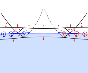
Previous works on shock refraction and RMI have mainly dealt with uniform incident shocks, perfectly planar or cylindrical. However, in practical applications, the incident shocks exhibit inherent non-uniformity and propagate with oscillations, giving rise to the spontaneous emergence of geometric singularities such as triple points and Mach stems (Gardner, Book & Bernstein Reference Gardner, Book and Bernstein1982; Lodato, Vervisch & Clavin Reference Lodato, Vervisch and Clavin2016; Mostert et al. Reference Mostert, Pullin, Samtaney and Wheatley2018a,Reference Mostert, Pullin, Samtaney and Wheatleyb), as depicted in figure 1. Upon encountering an interface, these non-uniform incident shocks inevitably seed perturbations that are subsequently amplified, even if the interface is initially uniform (Ishizaki & Nishihara Reference Ishizaki and Nishihara1997; Smalyuk et al. Reference Smalyuk2020; Velikovich et al. Reference Velikovich, Schmitt, Zulick, Aglitskiy, Karasik, Obenschain, Wouchuk and Cobos Campos2020). For instance, in the context of ICF, non-uniform laser illumination launches a non-spherical shock wave that undergoes a nonlinear transition, resulting in the formation of a faceted polyhedral shock consisting of incident shocks, triple points, Mach stems, and following reflected polar shocks (Gardner et al. Reference Gardner, Book and Bernstein1982; Thomas & Kares Reference Thomas and Kares2012). This faceted, non-uniform shock seeds perturbations for the acceleration phase of the target, inducing Rayleigh–Taylor instability and facilitating turbulent mixing that ultimately results in ignition failure (Thomas & Kares Reference Thomas and Kares2012; Smalyuk et al. Reference Smalyuk2020). Such interactions are complicated and it is imperative to conduct exploratory studies in order to elucidate the crucial processes involved.

Figure 1. Schematic diagram of non-uniform shocks: (a) a non-uniform shock with a smooth shock front; (b) a faceted non-uniform shock with inherent triple-shock configurations. The red arrows indicate the orientations of the shocks.
Ishizaki et al. (Reference Ishizaki, Nishihara, Sakagami and Ueshima1996) first numerically investigated the instability of a uniform interface accelerated by a non-uniform shock driven by a moving rippled piston. They reported that the evolution of this instability exhibits two distinct regimes, namely linear and nonlinear regimes, depending on the amplitude of the rippled piston. The linear regime occurs when the amplitude of the rippled piston is small and the non-uniform shock front is sinusoidal (see figure 1a). For this regime, Ishizaki et al. (Reference Ishizaki, Nishihara, Sakagami and Ueshima1996) proposed an analytical theory that considers both the impulsive acceleration induced by the non-uniform shock front and the continuous pressure perturbation behind the shock front. However, when the amplitude of the rippled piston increases, the initially sinusoidal shock front undergoes a transition to a faceted one characterized by ‘cusp-like structured shock’ (i.e. triple points and Mach stems) (see figure 1b). This phenomenon indicates the emergence of a nonlinear regime, which is characterized by the formation of irregular square-shaped perturbations on the interface. It was inferred that these square-shaped perturbations are induced by velocity impulses resulting from the passage of the ‘cusp-like structured shocks’. Such instabilities induced by non-uniform shocks are commonly referred to as Richtmyer–Meshkov-like (RM-like) instability in the literature (Velikovich Reference Velikovich2000; Nishihara et al. Reference Nishihara, Wouchuk, Matsuoka, Ishizaki and Zhakhovsky2010). Our recent shock tube experiments (Zou et al. Reference Zou, Liu, Liao, Zheng, Zhai and Luo2017) have also examined the RM-like instability, where a non-uniform shock with inherent triple-shock configurations is produced by diffracting a planar shock around a rigid cylinder. Of great interest, the incident triple-shock configuration imprints a central cavity on the interface, which exhibits a morphology similar to the square-shaped perturbations previously observed by Ishizaki et al. (Reference Ishizaki, Nishihara, Sakagami and Ueshima1996). Subsequently, Zhou (Reference Zhou2017a) has specially addressed this RM-like instability in his review article. More recently, Liao et al. (Reference Liao, Zhang, Chen, Zou, Liu and Zheng2019) experimentally examined the effects of the Atwood number (defined as  ${{{A}}{t}} = ({\rho _{_{0'}}} - {\rho _0})/({\rho _{_{0'}}} + {\rho _0})$ with
  ${\rho _{_{0}}}$ and
  ${\rho _{_{0'}}}$ being the initial densities of the light and heavy gases, respectively) on the perturbation growth of this RM-like instability. They concluded that the perturbation growth rate of this RM-like instability decreases as the Atwood number increases, which is fundamentally different from the results related to the classical RMI. However, the underlying physical mechanism behind this novel phenomenon remains unclear (He et al. Reference He, Peng, Li, Tian and Yang2023).
The aforementioned investigations have provided valuable insights into the flow physics of the RM-like instability. However, a comprehensive analytical theory that accounts for the scenarios of RM-like instability has yet to be developed due to the complexity introduced by triple-shock configurations. As depicted in figure 1(b), a triple-shock configuration consists of four discontinuities, namely a Mach stem, incident and reflected shocks, and a slipstream. The leading shock front comprises the Mach stem and incident shock, while the reflected shock originates from the triple point and travels transversely behind it (Lau-Chapdelaine & Radulescu Reference Lau-Chapdelaine and Radulescu2016). When a triple-shock configuration encounters an interface, both the leading shock front and the reflected shock successively interact with the interface. These interactions inevitably give rise to complex wave configurations and deposit velocity perturbations as well as baroclinic vorticity on the interface. Therefore, accurately predicting the velocity perturbation and vorticity deposition induced by triple-shock refraction is of great significance in uncovering the underlying physical mechanisms governing the RM-like instability. In addition, it is of great interest and importance to understand the wave configuration that occurs when a triple-shock configuration refracts at a planar interface. A definite answer to these questions requires a detailed and careful examination of the triple-shock refraction process, which motivates this work. The remainder of the paper is organized as follows. The numerical approach, experimental set-up and analytical method are presented in § 2. Detailed results and discussion regarding the flow features are provided in §§ 3 and 4. Finally, concluding remarks are summarized in § 5.
2. Methodology
According to our previous works (Zou et al. Reference Zou, Liu, Liao, Zheng, Zhai and Luo2017; Liao et al. Reference Liao, Zhang, Chen, Zou, Liu and Zheng2019), the incident triple-shock configuration is generated by diffracting a planar shock around a rigid cylinder. As indicated by Bryson & Gross (Reference Bryson and Gross1961) and Zou et al. (Reference Zou, Liu, Liao, Zheng, Zhai and Luo2017), the structure of the incident triple-shock configuration is determined by the Mach number of the incident planar shock, the diameter of the rigid cylinder, together with the distance that the diffracted shock travels downstream. In the present work, to eliminate the complexity induced by the variation of the structure of the incident triple-shock configuration, the Mach number of the incident planar shock is kept at  $M_{{i}} = 1.80$, the diameter of the rigid cylinder is kept at
  $d = 10$ mm and the distance between the centre of the rigid cylinder and the initial interface is kept at
  $l = 40$ mm.
2.1. Numerical approach
The numerical simulations are conducted using a compressible multicomponent Euler solver based on the finite volume method (Sun & Takayama Reference Sun and Takayama1999). In a quasiconservative form, the governing equations can be written as
 \begin{equation} \frac{{\partial {\boldsymbol{U}}}}{{\partial {{t}}}} + \frac{{\partial {\boldsymbol{F}}({\boldsymbol{U}})}}{{\partial {{x}}}} + \frac{{\partial {\boldsymbol{G}}({\boldsymbol{U}})}}{{\partial {{y}}}} = 0, \end{equation}
where  ${\boldsymbol {U}}$ represents the conserved variable,
  ${\boldsymbol {F}}({\boldsymbol {U}})$ and
  ${\boldsymbol {G}}({\boldsymbol {U}})$ are the convective fluxes in the
  $x$ and
  $y$ directions, respectively,
 \begin{equation}
U = \left( \begin{array}{@{}c@{}} {{\rho }}\\ {{\rho u}}\\ {{\rho v}}\\
{{\rho E}}\\ {{\rho }}{{{Y}}_s} \end{array} \right)\!,
\quad F = \left( \begin{array}{@{}c@{}} {{\rho u}}\\ {{\rho
}}{{{u}}^{{2}}}+p\\ {{\rho uv}}\\ ({{\rho E +
p}}){{u}}\\ {{\rho }}{{{Y}}_s}{{u}} \end{array}
\right)\!,\quad G = \left( \begin{array}{@{}c@{}} {{\rho v}}\\
{{\rho uv}}\\ {{\rho }}{{{v}}^{{2}}}+p\\ ({{\rho E +
p}}){{v}}\\ {{\rho }}{{{Y}}_s}{{v}} \end{array}
\right)\!,\end{equation}
\begin{equation}
U = \left( \begin{array}{@{}c@{}} {{\rho }}\\ {{\rho u}}\\ {{\rho v}}\\
{{\rho E}}\\ {{\rho }}{{{Y}}_s} \end{array} \right)\!,
\quad F = \left( \begin{array}{@{}c@{}} {{\rho u}}\\ {{\rho
}}{{{u}}^{{2}}}+p\\ {{\rho uv}}\\ ({{\rho E +
p}}){{u}}\\ {{\rho }}{{{Y}}_s}{{u}} \end{array}
\right)\!,\quad G = \left( \begin{array}{@{}c@{}} {{\rho v}}\\
{{\rho uv}}\\ {{\rho }}{{{v}}^{{2}}}+p\\ ({{\rho E +
p}}){{v}}\\ {{\rho }}{{{Y}}_s}{{v}} \end{array}
\right)\!,\end{equation}
where  $u$ and
  $v$ represent the velocity components in the
  $x$ and
  $y$ directions, respectively, and
  $\rho$ and
  $p$ represent the density and pressure. Here
  ${Y_s}$ stands for the mass fraction of the gas at one side of the interface, and the mass fraction of gas
  $b$ at the other side of the interface is
  ${Y_b} = 1 - {Y_s}$. The equation of state of the mixture is expressed as
  $p = \rho T( {{Y_s}{R_s} + {Y_b}{R_b}} )$, where
  ${R_s}$ and
  ${R_b}$ are the gas constants of gases
  $s$ and
  $b$, and
  $T$ is the temperature of the mixture. Here
  $E$ is the total energy of the mixture, defined as
  $E=Y_s e_s + Y_b e_b + (u^2 + v^2)/2$ where
  $e_s$ and
  $e_b$ are the internal energies of gases
  $s$ and
  $b$.
$b$.
The MUSCL (monotonic upstream-centred scheme for conservation laws)–Hancock scheme (Toro Reference Toro2009) is adopted to achieve the second-order accuracy in both temporal and spatial scales. The HLL (Harten–Lax–van Leer) Riemann solver (Sun & Takayama Reference Sun and Takayama2003) is employed for the approximation of the physical fluxes. An adaptive mesh refinement technique (Sun & Takayama Reference Sun and Takayama1999) is employed such that it deploys dense grids in flow regions with large density and velocity gradients, thereby resolving waves and interface evolutions elaborately. This solver has been proven reliable in previous works in capturing the complex shock structures and interface evolution, such as shock–obstacle interactions (Sun & Takayama Reference Sun and Takayama2003), shock reflections (Wang & Zhai Reference Wang and Zhai2020; Wang, Zhai & Luo Reference Wang, Zhai and Luo2022) and shock–interface interactions (Zhai et al. Reference Zhai, Si, Luo and Yang2011, Reference Zhai, Liang, Liu, Ding, Luo and Zou2018).
The computational domain is shown in figure 2(a). Due to the symmetric nature of the flow field, only the upper-half-plane  $(0 \leqslant {{x}} \leqslant 250\ {\text {mm}}{\text { and }} 0 \leqslant {{y}} \leqslant 50\ {\text {mm}})$ is considered. The rigid cylinder is centred at
  $x = 20$ mm on the symmetry axis, and the initial interface is situated at
  $x = 60$ mm. The left and right boundaries are set as inflow and outflow conditions, respectively, while the upper and lower boundaries
  $( {{{y = }}0 \text { and }y = \ 50\ {\text {mm}}} )$ are treated as reflection and symmetry conditions, respectively. To highlight the influence of acoustic impedances of the gases on the triple-shock refraction, four different types of fast–slow interfaces are considered in computations with light gas of nitrogen (
 ${\rm N}_2$) and heavy gases of air, carbon dioxide (
 ${\rm CO_2}$), krypton (Kr) and sulphur hexafluoride (
 ${\rm SF}_6$), respectively. The thermal properties of the test gases are given in table 1. Here the interfaces are characterized by the acoustic impedance ratios of gases across the interfaces defined as
  $Z_{{r}}=Z_{{0'}}/Z_{{0}}$, with
  $Z_{{0}}$ and
  $Z_{{0'}}$ being the acoustic impedances of the light and heavy gases, respectively.

Figure 2. (a) Schematic of the computational domain. (b) The grid convergence validation.
Table 1. Thermal properties of the test gases considered in the numerical simulations, including the gas combination, specific heat ratio ( $\gamma$), density (
 $\rho$), sound speed (a), acoustic impedance (
 $Z$) of the heavy gases at
  $T_0 = 293.15$ K and
  $p_0 = 101 325$ Pa, and the acoustic impedance ratio (
 $Z_{{r}}$) across the interface. The value of
  $\gamma$,
  $\rho$,
  $a$ and
  $Z$ of the light gas (
 ${\rm N}_2$) are 1.399, 1.164, 348.9 and 406.1, respectively.

To validate the numerical solver as well as check the grid convergence, a planar shock diffracting around a rigid cylinder is considered, in which three sets of uniform grids with initial mesh sizes of 0.4, 0.2 and 0.1 mm, respectively, are tested. The initial temperature  $T_0$ of 293.15 K and initial pressure
  $p_0$ of 101 325 Pa are employed. The pressure profiles along the horizontal symmetry axis of the flow field with different initial mesh sizes are given in figure 2(b). The results obtained by the grids with initial mesh sizes of 0.2 mm and 0.1 mm collapse together, indicating a reasonable convergence of grid resolutions. To ensure the accuracy and meanwhile to minimize the computation capacity, the initial mesh size of 0.2 mm is adopted and the finest mesh size of 25
  $\mathrm {\mu }$m is used where a greater density gradient exists. As depicted in figure 3(a), the instantaneous numerical schlieren of the diffracted non-uniform shock just before it encounters the interface is validated against the experimental shadowgraphy of Liao et al. (Reference Liao, Zhang, Chen, Zou, Liu and Zheng2019). The numerical simulation reproduces nearly all features of wave pattern as observed in the experiment and good agreement is achieved between them. Furthermore, the computed trajectories of the two triple points (
 ${\rm TP_1}$,
  ${\rm TP_2}$) are measured and compared with the experimental data of Liao et al. (Reference Liao, Zhang, Chen, Zou, Liu and Zheng2019), as depicted in figure 3(b). The comparisons appear substantially satisfactory for both the outer and inner triple-shock configurations, validating the accuracy of the numerical solver.

Figure 3. Validation of the numerical solver. (a) Comparison of the wave configuration of the diffracted non-uniform shock just before it encounters the initial interface. (b) Comparison of triple points trajectories of the diffracted non-uniform shock.
2.2. Experimental set-up
The experiments are conducted in a vertical shock tube with a cross-section of  $100~{\rm mm} \times 100$ mm, comprising of a driver section (1.60 m long), a driven section (4.22 m long), and a test section (0.305 m long). As illustrated in figure 4(a), a flat interface is created in the test section utilizing the membraneless method originally proposed by Jones & Jacobs (Reference Jones and Jacobs1997), which has already been verified for its feasibility and reliability in our previous works (Zou et al. Reference Zou, Liu, Liao, Zheng, Zhai and Luo2017; Liao et al. Reference Liao, Zhang, Chen, Zou, Liu and Zheng2019). The detailed description of the shock tube facility and the interface generation method can be found in Zou et al. (Reference Zou, Liu, Liao, Zheng, Zhai and Luo2017) and Liao et al. (Reference Liao, Zhang, Chen, Zou, Liu and Zheng2019). In this work, three different types of fast–slow interfaces are successfully generated with light gas of
  ${\rm N}_2$ and heavy gases of
  ${\rm CO_2}$, Kr and
  ${\rm SF}_6$, respectively. However, the
  ${\rm N}_2$–air interface is excluded in the experiments due to the negligible difference in densities between the two gases, which poses a great challenge for generating the interface. Figure 4(b) illustrates the schematic of wave configurations after a planar shock diffracts around a rigid cylinder. To capture the evolution of the wave patterns and the interface elaborately, a shadowgraph photographic system similar to that adopted by Zou et al. (Reference Zou, Liu, Liao, Zheng, Zhai and Luo2017) and Liao et al. (Reference Liao, Zhang, Chen, Zou, Liu and Zheng2019) is employed, as shown schematically in figure 4(a). A 500 W xenon lamp (XQW500, Chengdu Photoelectricity Limited) is used to illuminate the flow field, and the shadowgraph images are recorded by a high-speed video camera (Phantom V1610) with a frame rate of 52 000 frames per second. The exposure time of the camera is 1
  $\mathrm {\mu }$s and the spatial resolution of the image is approximately 0.27 mm pixel
 $^{-1}$. Two pressure transducers (Ch1, Ch2) located above the test section and spaced 100 mm apart are used to measure the shock speed and to trigger the data acquisition system.

Figure 4. (a) Schematic of the test section of the shock tube with shadowgraph system. (b) Schematic of wave configurations after the shock diffracts around the cylinder. Here,  ${\rm TP_1}$ and
  ${\rm TP_2}$, respectively, denote the outer and inner triple points; IS,
  ${\rm MS}_1$,
  ${\rm MS_2}$,
  ${\rm RS_1}$ and
  ${\rm RS_2}$ refer to the incident shock, the outer Mach stem shock, the central Mach stem, the reflected/transverse shock emanating from
  ${\rm TP_1}$ and
  ${\rm TP_2}$, respectively;
  ${\rm SL_1}$ and
  ${\rm SL}_2$ denote the slipstream emanating from
  ${\rm TP_1}$ and
  ${\rm TP_2}$, respectively.
2.3. Pressure-deflection shock polar
The utilization of pressure-deflection shock polar is highly advantageous for analysing flow phenomena involving complex shock interactions and shock refractions, thereby facilitating a more comprehensive understanding of the flow physics (Olejniczak, Wright & Candler Reference Olejniczak, Wright and Candler1997; Ben-Dor Reference Ben-Dor2007; Vasilev, Elperin & Ben-dor Reference Vasilev, Elperin and Ben-dor2008; Gounko Reference Gounko2017; Zhang et al. Reference Zhang, Li, Ji, Si and Yang2021; Bai & Wu Reference Bai and Wu2022). For a detailed description of shock polars and their applications, readers can refer to Ben-Dor (Reference Ben-Dor2007). In this study, the triple-shock refraction process is examined by employing shock polars. Moreover, the utilization of shock polars enables a quantitative assessment of the velocity perturbation and the deposition of vorticity during triple-shock refraction (Samtaney & Zabusky Reference Samtaney and Zabusky1994). Note that the shock polars and the equations they represent are based on the assumption of a planar shock, which implies a uniform flow immediately downstream. Hence, the shock polars provide only an approximate representation of the actual flow in scenarios involving curved shocks, and are accurate only within a limited region surrounding the point of shock intersection. Nonetheless, based on the numerous numerical and experimental studies performed so far, it seems reasonable to assume a planar shock when using shock polars (Olejniczak et al. Reference Olejniczak, Wright and Candler1997; Vasilev et al. Reference Vasilev, Elperin and Ben-dor2008; Gounko Reference Gounko2017; Zhang et al. Reference Zhang, Li, Ji, Si and Yang2021; Ji et al. Reference Ji, Li, Zhang, Si and Yang2022). Therefore, in this study, it is assumed that the shocks of the triple-shock configuration are planar in the vicinity of the triple point, although slight curvature exists.
3. Flow structures and characteristics
3.1. Features of the diffracted non-uniform shock
Before illustrating the flow physics of triple-shock refraction, it is necessary to elaborate on the general features of the diffracted non-uniform shock. Diffraction of a planar shock around a rigid cylinder is a classical problem in shock dynamics, and for a detailed analysis readers can refer to Bryson & Gross (Reference Bryson and Gross1961) and Chaudhuri, Hadjadj & Chinnayya (Reference Chaudhuri, Hadjadj and Chinnayya2011). As shown in figure 4(a), the leading shock front of the diffracted non-uniform shock consists of two pairs of triple points  $( {\rm T{P_1},\ T{P_2}} )$ and several shock segments, namely the planar incident shock (IS) and the curved Mach stem shocks
  $( {\rm M{S_1},\ M{S_2}} )$. There are two characteristic triple-shock configurations on both sides of the flow symmetry axis, originating from
  ${\rm TP_1}$ and
  ${\rm TP_2}$. The structures of the two triple-shock configurations are determined by the Mach number (
 $M$) and incidence angle (
 $\alpha$, defined as the angle with respect to the horizontal direction) of their leading shock fronts in the vicinity of the triple points. The variation of
  $M$ and
  $\alpha$ for each shock segment are extracted from the numerical simulations and presented in figures 5(a) and 5(b), respectively. The Mach number of
  ${\rm MS}_1$ decreases gradually from
  ${\rm TP_1}$ to
  ${\rm TP_2}$ due to the shock attenuation when diffracting around the cylinder. The Mach number of
  ${\rm MS_2}$ exceeds that of
  ${\rm MS}_1$ because of the collision of the two
  ${\rm MS}_1$ from opposite sides. The incidence angle for IS is maintained at zero. Subsequently, the incidence angle experiences a sudden jump upon crossing
  ${\rm TP_1}$ from IS to
  ${\rm MS}_1$ due to the shock interaction, then increases monotonically and reaches a local maximum value at
  ${\rm TP_2}$. From figure 5, both the shock Mach number and incidence angle exhibit a more pronounced variation when crossing
  ${\rm TP_2}$ compared with
  ${\rm TP_1}$, indicating a stronger and more stable triple-shock configuration originating from
  ${\rm TP_2}$. Therefore, in the subsequent sections, we focus on examining the refraction of the triple-shock configuration originating from
  ${\rm TP_2}$. The shock front parameters depicted in figure 5 will be used as input data for the theoretical analysis, which will be elaborated in detail in § 4.

Figure 5. Distribution of (a) the Mach number and (b) the incidence angle of the leading shock front of the non-uniform shock just before it encounters the initial interface.
3.2. Qualitative description of the triple-shock refraction process
3.2.1. Triple-shock refraction at a planar N $_2$–air interface

Figure 6 illustrates the refraction of the triple-shock configuration originating from  ${\rm TP_2}$ at a planar
  ${\rm N}_2$–air interface, where the numerical schlieren images and the schematics of the wave configurations are presented on the left- and right-hand sides, respectively. Due to the symmetric nature of the flow field, only the right-hand half of the entire wave configurations is displayed for clarity. The initial time, i.e.
  $t = 0\ \mathrm {\mu }$s, is defined as the moment when IS collides with the initial interface, and the corresponding wave configuration is shown in figure 6(a). As time proceeds, the outer Mach stem shock (
 ${\rm MS}_1$) first intersects the interface at point
  ${\rm IP_1}$ and undergoes primary regular refraction due to its relatively small incidence angle, generating a transmitted shock (
 ${\rm TS}_1$) and a reflected shock (
 ${\rm RS}_3$). A detailed enlargement of the flow field in the vicinity of
  ${\rm IP_1}$, as depicted in figure 6(b), reveals that the refraction of
  ${\rm MS}_1$ deposits positive baroclinic vorticity on the interface. At
  $t = 4\ \mathrm {\mu }$s, as shown in figure 6(c), the central Mach stem shock (
 ${\rm MS_2}$), the triple point (
 ${\rm TP_2}$) and the outer Mach stem shock (
 ${\rm MS}_1$) all intersect with the interface simultaneously. At this moment, the four shocks
  ${\rm RS_2}$,
  ${\rm TS}_1$,
  ${\rm MS_2}$ and
  ${\rm RS}_3$ coincide at a single point on the interface, mutually modifying each other and indicating a critical condition for the refracting shock system. As presented in figure 4,
  ${\rm MS_2}$ is almost parallel to the initial interface. Consequently, regular refraction of
  ${\rm MS_2}$ occurs upon encountering the initial interface. In conjunction with the refraction of
  ${\rm MS_2}$,
  ${\rm RS_2}$ interferes with
  ${\rm RS}_3$ from the opposite family at point
  ${\rm IP}_3$. This shock interaction generates
  ${\rm RS}_4$ and
  ${\rm RS}_5$ to match the flow field. At the same time,
  ${\rm RS}_5$ intersects with the evolving interface segment previously shocked by
  ${\rm MS}_1$ at point
  ${\rm IP}_4$, resulting in secondary shock refraction and forming a reflected shock (
 ${\rm RS_6}$) and a transmitted shock (
 ${\rm TS_2}$). A zoomed-in view of the flow field near
  ${\rm IP}_4$, as depicted in figure 6(d), reveals that the secondary refraction of
  ${\rm RS}_5$ deposits negative vorticity on the interface. That is to say, the secondary refraction of
  ${\rm RS}_5$ suppresses vorticity originally deposited by the primary refraction of
  ${\rm MS}_1$ on the interface.

Figure 6. Sequences of numerical schlieren frames and schematic diagrams illustrating the evolution of triple-shock refraction at a  ${\rm N}_2$–
 ${\rm air}$ interface. The red arrows indicate the orientations of the shocks. Here (a)
  $t=0\ \mathrm {\mu }$s, (b)
  $t=2\ \mathrm {\mu }$s, (c)
  $t=4\ \mathrm {\mu }$s and (d)
  $t=10\ \mathrm {\mu }$s.
In addition to the deposition of baroclinic vorticity, the triple-shock refraction also imparts a longitudinal velocity perturbation on the interface. As previously mentioned, the shock Mach number and incidence angle exhibit pronounced variations along the leading shock front of the incident triple-shock configuration, resulting in a non-uniform impulsive acceleration of the interface. Recalling that  ${\rm MS_2}$ is stronger and has a relatively smaller incidence angle than
  ${\rm MS}_1$ (see figure 5); this implies that the central interface segment shocked by
  ${\rm MS_2}$ immediately gains a larger velocity after the passage of the leading shock front, thereby imparting a velocity perturbation on the interface. However, following the passage of the leading shock front, the secondary refraction of
  ${\rm RS}_5$ at the evolving interface segment shocked by
  ${\rm MS}_1$ further accelerates the interface segment and partially balances the longitudinal velocity perturbation. Consequently, the secondary refraction of
  ${\rm RS}_5$ may effectively suppress the growth of interface perturbation by concurrently inhibiting vorticity deposition and balancing velocity perturbations on the interface. Note that in the theoretical analysis of Ishizaki et al. (Reference Ishizaki, Nishihara, Sakagami and Ueshima1996), only the velocity perturbation imparted by the leading shock front of a non-uniform shock was considered. However, based on the above results, both the leading shock front and the reflected shock travelling transversely behind it play crucial roles in the interface evolution. The quantitative assessment of the contribution of the reflected shock to the interface evolution will be presented in § 4.3.1.
In concurrence with the perturbation of the interface, a complex pattern of reflected waves is generated, which comprises multiple curved shocks ( ${\rm RS}_3$,
  ${\rm RS}_4$,
  ${\rm RS_7}$ and
  ${\rm RS_8}$), a triple point (
 ${\rm TP_4}$), a shock intersection point (
 ${\rm IP}_4$) as well as transverse shocks (
 ${\rm RS_2}$,
  ${\rm RS}_5$,
  ${\rm RS_6}$) and slipstreams, as shown in figure 6(d). Of great interest, a transmitted triple-shock configuration is identified in the transmitted gas, comprising of shocks
  ${\rm TS}_1$,
  ${\rm MS_3}$,
  ${\rm TS_2}$, as well as a slipstream
  ${\rm SL_3}$ emanating from the transmitted triple point
  ${\rm TP_3}$. For convenience, this type of triple-shock refraction with the formation of a transmitted tripe-shock configuration is referred to as a type A triple-shock refraction.
3.2.2. Effects of acoustic impedances on the triple-shock refraction
When  $Z_{{r}}$ is increased, various patterns of refracted wave configurations are obtained. Figure 7(a,b) demonstrates the refractions of the triple-shock configuration at
  ${\rm N}_2$–
 ${\rm CO}_2$ and
  ${\rm N}_2$–Kr interfaces. In general, the evolution of the wave configurations exhibits similar characteristics to those observed in the case of a
  ${\rm N}_2$–
 ${\rm air}$ interface, with discrepancies observed only in the transmitted wave configurations as shown in figures 6(d) and 7(a,b). Notably, the numerical schlieren images shown in figure 7(avi) and 7(bvi) clearly display a transmitted four-shock configuration consisting of four shocks (
 ${\rm MS_3}$,
  ${\rm TS}_1$,
  ${\rm TS_2}$ and
  ${\rm TS_3}$) and a slipstream (
 ${\rm SL_3}$). These five discontinuities meet at a single point
  ${\rm TP_3}$, contradicting von Neumann's three-shock theory (Von Neumann Reference Von Neumann1943, Reference Von Neumann1945). Note that the discrepancy between von Neumann's three-shock theory and Mach reflection configurations was first experimentally detected by White (Reference White1952) in weak shock reflection and subsequently confirmed by numerous experiments (Zaslavsky & Safarov Reference Zaslavsky and Safarov1975; Henderson & Siegenthaler Reference Henderson and Siegenthaler1980; Colella & Henderson Reference Colella and Henderson1990; Skews & Ashworth Reference Skews and Ashworth2005). These discrepancies are commonly named the von Neumann paradox. To resolve the von Neumann paradox, Guderley (Reference Guderley1947) and Vasilev (Reference Vasilev1999) developed a four-wave theory by introducing a Prandtl–Meyer expansion fan into the triple-shock configuration. In addition, Vasilev et al. (Reference Vasilev, Elperin and Ben-dor2008) reconsidered the von Neumann paradox using shock polar analysis and predicted two distinct four-wave configurations: Guderley reflection and Vasilev reflection. However, the four-shock configuration identified in this study is distinctly different from the four-wave configurations predicted by Vasilev et al. (Reference Vasilev, Elperin and Ben-dor2008). The shadowgraph images shown in figure 7(av) and 7(bv) provide experimental evidence for this four-shock configuration. To the authors’ knowledge, such a four-shock configuration has not been reported before. Specifically, this type of triple-shock refraction is referred to as type B triple-shock refraction, and the detailed wave configurations are schematically depicted in figure 8(a). Considering the similarity in reflected wave configurations between type A and type B triple-shock refraction, as well as the symmetric nature of the flow field, only the right-hand half of the flow regions within the transmitted gas is illustrated in figure 8(a) for clarity.

Figure 7. Sequences of numerical schlieren images and experimental shadowgraphs showing the evolution of triple-shock refractions at interfaces with various combinations of acoustic impedances. Here (a)  ${\rm N}_2/{\rm CO}_2$, (b)
  ${\rm N}_2/{\rm Kr}$ and (c)
  ${\rm N}_2/{\rm SF}_6$.

Figure 8. Detailed schematics illustrating the flow field of type B and type C triple-shock refractions.
Regarding the case of  ${\rm N}_2$–
 ${\rm SF}_6$ interface, the numerical schlieren image presented in figure 7(cvi) clearly demonstrates a transmitted four-wave configuration that includes a Prandtl–Meyer expansion fan (EW), in addition to the classical triple-shock configuration. This transmitted four-wave configuration is similar to the wave configuration of both the Guderley reflection and the Valisev reflection (Vasilev et al. Reference Vasilev, Elperin and Ben-dor2008). Note that EW originating from
  ${\rm TP_3}$ slightly complicates the flow by impacting the interface in the backward direction and generating a reflected shock
  ${\rm RS_9}$. This type of triple-shock refraction is classified as type C triple-shock refraction. Unfortunately, the experimental identification of the transmitted four-wave configuration is hindered by both the strong diffusion of the
  ${\rm N}_2$–
 ${\rm SF}_6$ interface and the narrow space between the interface and the transmitted shocks. Figure 8(b) illustrates the detailed wave configuration and flow field resulting from type C triple-shock refraction for comparison, highlighting the differences in the flow field near
  ${\rm TP_3}$.
4. Theoretical results and discussion
In this section, analytical models will be developed to solve the wave angles and flow properties behind the waves associated with the process of triple-shock refraction. The input data used in the analytical model includes the parameters of the leading shock front of the incident triple-shock configuration, along with the thermal properties of gases on both sides of the initial interface. Specifically, the analysis decomposed the triple-shock refraction process into five fundamental processes, namely: analytical characterization of the incident triple-shock configuration; solution of the primary shock refraction; solution of the shock–shock interaction; solution of the secondary shock refraction; solution of the transmitted wave configuration. Once the flow properties in different regions illustrated in figures 6(d) and 8 have been determined, it becomes feasible to quantitatively evaluate the effects of velocity perturbation and baroclinic vorticity induced by the triple-shock refraction. Moreover, the flow properties of the regions surrounding the transmitted triple point can be utilized to draw shock polars for the transmitted wave configuration, thereby providing valuable insights into the mechanisms that determine the pattern of the transmitted wave.
In the subsequent analysis, we use  $\boldsymbol {V}$ and
  $M$ to represent the velocity and Mach number of the gas, respectively. The angle of the shock wave with respect to its upstream flow direction (shock angle) is denoted by
  $\beta$. The flow deflection angle across a shock or an expansion fan is denoted by
  $\delta$, with positive values for anticlockwise deflections. The gases are considered as calorically and thermally perfect. The conservation relationships across various types of discontinuities, including oblique shock wave, expansion waves and slipstream, are universal and can be found in Anderson (Reference Anderson2001).
4.1. Analytical solution of the triple-shock refraction
4.1.1. Analytical characterization of the incident triple-shock configuration
The analysis of the triple-shock refraction begins with the characterization of the incident triple-shock configuration. The flow field around  ${\rm TP_2}$ depicted in figure 4(a) is appropriately magnified and presented in figure 9. By attaching a frame of reference to
  ${\rm TP_2}$, the unsteady triple-shock configuration is transformed into a pseudosteady one, and all flow properties that are frame of reference dependent are appropriately marked. Figure 9 shows that four discontinuities, namely
  ${\rm MS}_1$,
  ${\rm RS_2}$,
  ${\rm MS_2}$ and
  ${\rm SL}_2$, coincide at
  ${\rm TP_2}$ and divide the flow field into four regions (i.e. regions (0)–(3)). Similar to von Neumann's three-shock theory (Von Neumann Reference Von Neumann1945), the flow solutions in regions (0)-(3) are assumed to be uniform, disregarding the influence of shock curvatures. Consequently, the flow field in the vicinity of
  ${\rm TP_2}$ can be solved by applying the conservation relationships across the oblique shocks and appropriate matching conditions across
  ${\rm SL}_2$.

Figure 9. (a) Schematic diagram and (b) shock-polar solution of the incident triple-shock configuration. The solid points represent the solution points, and the hollow circles denote the sonic points.
To characterize the incident triple-shock configuration depicted in figure 9(a), only three parameters of the leading shock front are required, namely, the Mach numbers ( $M{_{{i}}}$,
  $M{_{{m}}}$) of
  ${\rm MS}_1$ and
  ${\rm MS_2}$, along with the incidence angle (
 $\alpha _{{i}}$) of
  ${\rm MS}_1$. In the frame of reference attached to
  ${\rm TP_2}$, the oncoming flow Mach number (
 ${M_0}( {{{\rm T}}{{{\rm P}}_2}} )$) in zone (0) and the shock angle (
 ${\beta _{{i}}}( {{{\rm T}}{{{\rm P}}_{{2}}}} )$) of
  ${\rm MS}_1$ are derived as
 \begin{equation} \left. \begin{array}{c@{}} {M_0}{{\rm (T}}{{{\rm P}}_2}) = M{_{{i}}}/\cos (\chi + {\alpha _i})\\ {\beta _{{i}}}{{\rm (T}}{{{\rm P}}_2}) = \dfrac{ {{\rm \pi}}}{ 2} - {\alpha _{{i}}} - \chi \end{array} \right\}\!,\end{equation}
where  $\chi$ represents the trajectory angle of
  $\textrm{TP}_2$, which is defined as the angle with respect to the
  $x$-axis direction.
Following the three-shock theory, we apply oblique shock relations near  $\textrm {TP}_2$. These relations are used across
  $\textrm {MS}_1$ for weak solution, across
  $\textrm {RS}_2$ for weak solution normally but only when
  ${M_2}{\textrm {(T}}{{\textrm {P}}_2}) < 1$ for strong solution. Additionally, these relations are applied across
  $\textrm {MS}_2$ for strong solution.
The matching conditions across  $\textrm {SL}_2$ separating regions (2) and (3) are
 \begin{equation} \left. \begin{array}{c@{}} {p_3}/{p_0} = {p_2}/{p_0} = (\,{p_2}/{p_1})(\,{p_1}/{p_0})\\ {\delta _3}( {{{\rm T}}{{{\rm P}}_{{2}}}} ) = {\delta _1}( {{{\rm T}}{{{\rm P}}_{{2}}}} ) \pm {\delta _2}( {{{\rm T}}{{{\rm P}}_{{2}}}} ) \end{array} \right\}\!, \end{equation}
where  ${\delta _3}( {{\textrm {T}}{{\textrm {P}}_{{2}}}} ) = {\delta _1}( {{\textrm {T}}{{\textrm {P}}_{{2}}}} ) - {\delta _2}( {{\textrm {T}}{{\textrm {P}}_{{2}}}} )$ for a ‘standard’ triple-shock configuration and
  ${\delta _3}( {{\textrm {T}}{{\textrm {P}}_{{2}}}} ) = {\delta _1}( {{\textrm {T}}{{\textrm {P}}_{{2}}}} ) + {\delta _2}( {{\textrm {T}}{{\textrm {P}}_{{2}}}} )$ for a ‘non-standard’ triple-shock configuration.
To quantify the triple-shock configuration surrounding  $\textrm {TP}_2$, we measure the shock front parameters defined in figure 9(a) from figures 5(a) and 5(b). The resulting values for
  $\textrm {MS}_1$ are
  $M{_{{i}}} = 1.62$ and
  ${\alpha }_{{i}} = 14.4^\circ$, while the value for
  $\textrm {MS}_2$ is
  $M_{{m}} = 1.83$. Figure 9(b) illustrates a shock-polar solution of the incident triple-shock configuration, where positive angles correspond to anticlockwise flow deflections. The numbered regions in figure 9(a) correspond to the numbered points of the shock polar intersections. The oncoming flow shock polar is determined by the oncoming flow Mach number
  ${M_0}({\textrm {T}}{{\textrm {P}}_2}) = 1.94$, originating from the origin. Point (1) lies on the oncoming flow shock polar at
  ${\delta _1}({\textrm {T}}{{\textrm {P}}_2}) = 20.3^\circ$. The flow parameters immediately behind
  ${\textrm {M}}{{\textrm {S}}_1}$ (i.e. region (1)) are utilized to determine the reflection shock polar for region (1), which originates from point (1). The intersection point between the shock polar for region (1) and the oncoming flow shock polar, labelled (2) and (3), represents the theoretical solution for the flow states in regions (2) and (3), respectively. The theoretical pressure ratio of 3.74 in regions (2) and (3) agrees well with the computed value of 3.73. Additionally, the theoretical value of the triple point trajectory angle (
 $\chi$) is approximately
  $18.9^\circ$, which also agrees satisfactorily with the numerical value (
 $18.6^\circ$) obtained from linearly fitting the trajectory (as displayed in figure 4b) of
  $\textrm {TP}_2$. Thus, the shock polars can be used to distinguish between different types of shock reflection and quantify the strength and orientation of
  $\textrm {RS}_2$. The reflected shock (
 $\textrm {RS}_2$) and the shear layer (
 $\textrm {SL}_2$), obtained from the shock polar analysis, are superimposed on the numerical contour of the normalized temperature
  ${{T/}}{{{T}}_0}$ in figure 10 for comparison, showing a good agreement. Note that this type of shock reflection should be categorized as von Neumann reflection (Ben-Dor Reference Ben-Dor2007; Vasilev et al. Reference Vasilev, Elperin and Ben-dor2008; Yang, Li & Wu Reference Yang, Li and Wu2013), since the solution of the three-shock theory is ‘non-standard’ where
  ${\delta _3}( {{\textrm {T}}{{\textrm {P}}_{{2}}}} ) = {\delta _1}( {{\textrm {T}}{{\textrm {P}}_{{2}}}} ) + {\delta _2}( {{\textrm {T}}{{\textrm {P}}_{{2}}}} )$. In other words, the oncoming flow in region (0) is deflected in the same direction successively by
  $\textrm {MS}_1$ and
  $\textrm {RS}_2$.

Figure 10. Comparison between the analytical wave configuration (denoted by dashed lines) and the numerical contour of the normalized temperature.
4.1.2. Solution of the primary shock refraction
As previously shown in figures 6(b) and 6(c), shocks  $\textrm {MS}_1$ and
  $\textrm {MS}_2$ intersect with the initial interface successively, resulting in regular shock refractions. Only the relations related to the refraction of
  $\textrm {MS}_1$ are derived below, as those associated with the refraction of
  $\textrm {MS}_2$ are similar. The appropriate parts of the resulting wave configurations, generated by the refraction of
  $\textrm {MS}_1$ (see figures 6b), are enlarged and schematically illustrated in figure 11(a). The frame of reference is attached to
  $\textrm {IP}_1$ where
  $\textrm {MS}_1$,
  $\textrm {RS}_3$ and
  $\textrm {TS}_1$ intersect at the interface, and all the flow properties that are frame of reference dependent are appropriately marked. Here,
  $\gamma _0$ and
  ${\gamma '_0}$ represent the ratios of specific heats in the incident and transmitted gases, respectively. Here
  ${p_0}$ and
  ${\rho _{0'}}$, respectively, denote the initial pressure and density of the flow in region (
 $0'$).

Figure 11. (a) Schematic illustration of the primary refraction of  $\textrm {MS}_1$ at the initial interface and (b) shock-polar solution of the primary refraction of
  $\textrm {MS}_1$ at a
  $\textrm {N}_2$–Kr interface. The solid points represent the solution points.
According to the shock refraction law (Henderson Reference Henderson2014), the incident and transmitted shocks must propagate at the same velocity along the interface. As a result, the parameters of  $\textrm {TS}_1$ can be related to those of
  $\textrm {MS}_1$ using the following expression:
 \begin{equation} M{{\rm (T}}{{{\rm S}}_{{1}}}{{\rm )}}a'_0/\sin {\alpha ({{\rm T}}{{{\rm S}}_1})} = M{_{{i}}}{a_0}/\sin {\alpha _i}, \end{equation}
where  $M({\textrm {T}}{{\textrm {S}}_{{1}}})$ and
  $\alpha ({\textrm {T}}{{\textrm {S}}_1})$ are the Mach number and angle of incidence of
  $\textrm {TS}_1$, respectively;
  ${a_0} = \sqrt {{\gamma _0}{p_0}/{\rho _0}}$ and
  ${a'_0} = \sqrt { {\gamma '_0}{p_0}/\rho'_0}$ are, respectively, the initial sound speeds of the incident gas in region (0) and the transmitted gas in region (
 $0'$). In the frame of reference attached to
  $\textrm {IP}_1$, the Mach numbers of the oncoming flows in regions (0) and (
 $0'$) are
  ${M_0}({\textrm {I}}{{\textrm {P}}_1})$ and
  ${M_{0'}}({\textrm {I}}{{\textrm {P}}_1})$, respectively, and are derived as
 \begin{equation} \left. \begin{array}{c@{}} {M_0}({{\rm I}}{{{\rm P}}_1}) = M{_{{i}}}/\sin {\alpha _i}\\ {{M}_{0'}}({{\rm I}}{{{\rm P}}_1}) = M{{\rm (T}}{{{\rm S}}_{{1}}}{{\rm )}}/\sin {\alpha ({{\rm T}}{{{\rm S}}_1})} = M{_{{i}}}({a_0}/a'_0){ / }\sin {\alpha _i} \end{array} \right\}\!.\end{equation}
The shock angle of  $\textrm {MS}_1$ with respect to the oncoming flow in region (0) is
 \begin{equation} {\beta _{1}}({{\rm I}}{{{\rm P}}_1}) = \frac{{\rm \pi} }{2} - {\alpha _{{i}}} .\end{equation}
The oblique shock relations are applied, in the vicinity of  $\textrm {IP}_1$, across
  $\textrm {MS}_1$,
  $\textrm {RS}_3$ and
  $\textrm {TS}_1$. In addition, the matching conditions across the shocked interface
  ${m'}$ separating regions (4) and (5) are
 \begin{equation} \left. \begin{array}{c@{}} (\,{p_4}/{p_1})(\,{p_1}/{p_0}) = {p_5}/{p_0}\\ {\delta _1}( {{{\rm I}}{{{\rm P}}_1}} ) - {\delta _4}( {{{\rm I}}{{{\rm P}}_1}} ) = {\delta _5}( {{{\rm I}}{{{\rm P}}_1}} ) \end{array} \right\}\!.\end{equation}
Figure 11(b) presents the shock-polar solution of the primary refraction of  $\textrm {MS}_1$ for the case of
  $\textrm {N}_2$–Kr interface. The shock polars for region (0) and (
 ${0'}$) are determined by the oncoming flow conditions
  ${M_0}({\textrm {I}}{{\textrm {P}}_1}) = 6.51, {\gamma _0} = 1.399$ and
  ${M_{0'}}({\textrm {I}}{{\textrm {P}}_1}) = 10.34, {\gamma _{0'}} = 1.661$, respectively. Point (1) is located on the oncoming shock polar for region (0) at the position of
  ${\delta _1}({\textrm {I}}{{\textrm {P}}_1}) = 7.32^\circ$. With the pressure ratio fixed, the Mach number in region (1),
  ${M_1}({\textrm {I}}{{\textrm {P}}_1}) = 5.37$ is uniquely determined, and the shock polar for region (1) can be drawn originating from point (1). Points (4) and (5) on the shock polar diagram have a pressure ratio of 3.81, which is exactly the same as the numerical value. Therefore, the shock polars can be used to quantify the strength of both the reflected and transmitted shocks (
 $\textrm {RS}_3$ and
  $\textrm {TS}_1$) as well as their incidence angles. As shown in figure 12, the analytical reflected shock (
 $\textrm {RS}_3$), transmitted shock (
 $\textrm {TS}_1$) and the shocked interface (
 ${m'}$) coincide with the numerical contour of the normalized temperature
  $T/{T_0}$.

Figure 12. Comparison of wave configurations and interface between analytical prediction (denoted by dashed lines) and numerical result for the primary refraction of  $\textrm {MS}_1$ at a
  $\textrm {N}_2\unicode{x2013}\textrm {Kr}$ interface.
Generally, the velocity of the doubly shocked flow in region (4) is lower than that of the flow in region (5), which has only been shocked by  $\textrm {TS}_1$, resulting in a shear across the interface (Samtaney & Zabusky Reference Samtaney and Zabusky1994). Consequently, the refraction process of
  $\textrm {MS}_1$ deposits baroclinic vorticity on the interface. By integrating the velocity along a contour with length
  $\textrm {d}{s}'$ parallel to the primary shocked interface and infinitesimally thin perpendicular to it, the circulation per unit length (CPUL) of the shocked interface (
 ${m'}$) can be obtained as
 \begin{equation} {\varGamma '_{{m'}}} = \frac{ {{\rm d}\varGamma_{{m'}}}}{ {{\rm d}{s}'}} = {V_{5t}} - {V_{4t}} ,\end{equation}
where  $V_{4t}$ and
  $V_{5t}$ denote the velocities tangential to
  ${m'}$ in the incident gas and the transmitted gas, respectively. Furthermore, (4.7) can be multiplied by the geometric factor
  $\textrm {d}{s}'/\textrm {d}{s} = [\cos {\alpha _i}/\cos ({\alpha _i}-{\delta _5}({\textrm {I}}{{\textrm {P}}_1})]$ to yield the CPUL with respect to the initial interface
  $m$:
$m$:
 \begin{equation} {\varGamma '_{{m}}} = \frac{ {{\rm d}\varGamma_{{m}}}}{ {{\rm d}{s}}} = ({V_{5t}} - {V_{4t}})\frac{{\cos {\alpha _i}}}{{\cos ({\alpha _i} - {\delta _5}({{{{\rm IP}}}_1}))}}.\end{equation}
Samtaney & Zabusky (Reference Samtaney and Zabusky1994) utilized an asymptotic method to provide a first-order estimation of (4.8), and proposed the SZ model, which is formulated as follows:
 \begin{align} {\varGamma '_{{m}, {SZ}}}&=\frac{ {{\rm d}\varGamma_{{m}}}}{ {{\rm d}s}} = \frac{ {2{\gamma _c}^{1/2}}}{ {{\gamma _c} + 1}}(1 - {\eta ^{ - {1}/{2}}})\sin {\alpha _i}(1 + M{({{\rm M}}{{{\rm S}}_1})^{ - 1}}\nonumber\\ &\quad + 2M{({{\rm M}}{{{\rm S}}_1})^{ - 2}})(M({{\rm M}}{{{\rm S}}_1}) - 1)\sqrt {\frac{ {{p_0}}}{ {{\rho _0}}}}, \end{align}
where  ${\gamma _c} = ({\gamma _0} + {\gamma _{0'}})/2$ and
  $\eta = {\rho _{0'}}/{\rho _0}$ denote the characteristic specific heat ratio and the density ratio of the preshocked gases across the interface, respectively.
4.1.3. Solution of the shock–shock interaction
The flow field surrounding  $\textrm {IP}_3$, where
  $\textrm {RS}_2$ and
  $\textrm {RS}_3$ interfere, is illustrated in figure 13(a). By attaching a frame of reference to
  $\textrm {IP}_3$, all the flow properties are appropriately marked. Prior to solving the flow field, the velocity of
  $\textrm {IP}_3$ with respect to region (1) should be determined. Considering that the wave configuration around
  $\textrm {IP}_3$ retains its structure as it evolves, i.e.
  $\textrm {RS}_2$ and
  $\textrm {RS}_3$ proceed at the same velocity with respect to region (1) along the trajectory of
  $\textrm {IP}_3$, the following geometric relations hold:
 \begin{equation} | {{{\boldsymbol{V}}_{{{I}}{{{P}}_3}}} - {{\boldsymbol{V}}_1} } | = \frac{ {{M}({{\rm R}}{ {{\rm S}}_2}){a_1}}}{{\sin (\alpha ({{\rm R}}{{{\rm S}}_2}) - \varepsilon )}} = \frac{ {{M}({{\rm R}}{{{\rm S}}_3}){a_1}}}{ {\sin \varepsilon }} ,\end{equation}
where  $\varepsilon$ is the unknown parameter that represents the trajectory angle of
  $\textrm {IP}_3$ with respect to
  $\textrm {RS}_3$ (see figure 13a), and the flow parameters
  ${M}({\textrm {R}}{{\textrm {S}}_2})$,
  ${M}({\textrm {R}}{{\textrm {S}}_3})$,
  $\alpha ({\textrm {R}}{{\textrm {S}}_2})$,
  ${{\boldsymbol {V}}_{{1}}}$ and
  $a_1$ are known.

Figure 13. (a) Schematic illustration of the interaction between  $\textrm {RS}_2$ and
  $\textrm {RS}_3$ and (b) shock-polar solution of the interaction between
  $\textrm {RS}_2$ and
  $\textrm {RS}_3$ involved in the triple-shock refraction at a
  $\textrm {N}_2$–Kr interface. The solid points represent the solution points.
In the frame of reference attached to  $\textrm {IP}_3$, the oncoming flow parameters in region (1) can be expressed as
 \begin{equation} \left.\begin{array}{c@{}} {M_1}({{\rm I}}{{{\rm P}}_3}) = \dfrac{ {{M}({{\rm R}}{{{\rm S}}_2})}}{ {\sin (\alpha ({{\rm R}}{{{\rm S}}_2}) - \varepsilon )}}\\ {\beta _2}({{\rm I}}{{{\rm P}}_3}) = \alpha ({{\rm R}}{{{\rm S}}_2}) - \varepsilon \\ {\beta _4}({{\rm I}}{{{\rm P}}_3}) = \varepsilon \end{array} \right\}\!.\end{equation}
 The oblique shock relations are applied, in the vicinity of  $\textrm {IP}_3$, across
  $\textrm {RS}_2$,
  $\textrm {RS}_3$,
  $\textrm {RS}_4$ and
  $\textrm {RS}_5$, respectively. In addition, the matching conditions across
  $\textrm {SL}_5$ separating regions (8) and (9) are as follows:
 \begin{equation} \left. \begin{array}{c@{}} (\,{p_9}/{p_2})(\,{p_2}/{p_1}) = (\,{p_{8}}/{p_4})(\,{p_4}/{p_1}) \\ {\delta _2}( {{{\rm I}}{{{\rm P}}_3}} ) - {\delta _9} ( {{{\rm I}}{{{\rm P}}_3}} ) = {\delta _{8}}( {{{\rm I}}{{{\rm P}}_3}} ) - {\delta _4}( {{{\rm I}}{{{\rm P}}_3}} ) \end{array} \right\}\!.\end{equation}
 The shock polars depicted in figure 13(b) illustrate the interaction between  $\textrm {RS}_2$ and
  $\textrm {RS}_3$ for the
  $\textrm {N}_2$–Kr interface case. State (1) at which
  $p/p_1=1$,
  ${\delta _1}{\textrm {(I}}{{\textrm {P}}_3}) = 0$, is located at the origin. The oncoming flow shock polar for region (1) is determined by the oncoming flow Mach number
  ${M_1}({\textrm {I}}{{\textrm {P}}_3}) = 4.20$. The points (2) and (4) are located on the oncoming flow shock polar at the locations of
  ${\delta _2}({\textrm {I}}{{\textrm {P}}_3}) = - 2.69^\circ$ and
  ${\delta _4}({\textrm {I}}{{\textrm {P}}_3}) = 2.43^\circ$, respectively. With the pressure ratios
  ${p_2}/{p_1} = 1.32$ and
  ${p_4}/{p_1} = 1.29$ fixed, the Mach numbers in regions (2) and (4),
  ${M_2}({\textrm {I}}{{\textrm {P}}_3}) = 3.98$ and
  ${M_4}({\textrm {I}}{{\textrm {P}}_3}) = 4.00$ can be uniquely determined. Consequently, the shock polars for regions (2) and (4) can be drawn originating from point (2) and (4) correspondingly. Points (8) and (9) should coincide at the intersection of shock polars for regions (2) and (4). Note that points (8) and (9) on the shock polar diagram have a pressure ratio of 1.67, which agrees well with the calculated value of 1.63.
4.1.4. Solution of the secondary shock refraction
As previously mentioned,  $\textrm {RS}_5$ intersects and interacts with
  ${m'}$ at
  $\textrm {IP}_4$. This intersection leads to a secondary shock refraction and deposits additional baroclinic vorticity on the interface. The resulting wave configuration from the secondary shock refraction is illustrated in figure 14(a), with the frame of reference being attached to
  $\textrm {IP}_4$, and all the flow properties, which are frame of reference dependent are appropriately marked. It should be noted that
  ${m'}$ is evolving and not vorticity-free. This differs from the aforementioned primary refractions of
  $\textrm {MS}_1$ and
  $\textrm {MS}_2$, where the interface
  $m$ is initially stationary and vorticity-free.

Figure 14. (a) Schematic illustration of the secondary refraction of  $\textrm {RS}_5$ and (b) shock-polar solution of the secondary refraction of
  $\textrm {RS}_5$ involved in the triple-shock refraction at a
  $\textrm {N}_2$–Kr interface. The solid points represent the solution points.
In the frame of reference attached to  $\textrm {IP}_4$, the flow parameters in zones (4) and (5) can be expressed as
 \begin{equation} \left. \begin{array}{c@{}} {M_4}({{\rm I}}{{{\rm P}}_4}) = {M}({{\rm R}}{{{\rm S}}_5})/\sin (\alpha ({{\rm R}}{{{\rm S}}_5}) + {\delta _4}({{\rm I}}{{{\rm P}}_1}))\\ {M_5}({{\rm I}}{{{\rm P}}_4}) = {M_4}({{\rm I}}{{{\rm P}}_4})({a_4}/{a_5})\\ {\beta _8}({{\rm I}}{{{\rm P}}_4}) = \alpha ({{\rm R}}{{{\rm S}}_5}) + {\delta _4}({{\rm I}}{{{\rm P}}_1}) \end{array} \right\}\!,\end{equation}
where  ${M}(\textrm {RS}_{5} )$,
  $\alpha ({\textrm {R}}{{\textrm {S}}_5})$,
  ${\delta _4}({\textrm {I}}{{\textrm {P}}_1})$,
  ${a_4}$ and
  ${a_5}$ are known.
The oblique shock relations are applied, in the vicinity of  $\textrm {IP}_4$, across
  $\textrm {RS}_5$,
  $\textrm {RS}_6$ and
  $\textrm {TS}_2$, respectively. In addition, the matching conditions across the secondary shocked interface (
 ${m''}$) separating regions (10) and (12) are
 \begin{equation} \left. \begin{array}{c@{}} (\,{p_8}/{p_4})(\,{p_{10}}/{p_8}) = {p_{12}}/{p_5} \\ {\delta _8}( {{{\rm I}}{{{\rm P}}_4}} ) - {\delta _{10}} ( {{{\rm I}}{{{\rm P}}_4}} ) = {\delta _{12}}( {{{\rm I}}{{{\rm P}}_4}} ) \end{array} \right\}\!.\end{equation}
Figure 14(b) illustrates the shock-polar solution of the secondary shock refraction of  $\textrm {RS}_5$ for the case of the
  $\textrm {N}_2$–Kr interface. The oncoming flow shock polars for regions (4) and (5) are determined by
  ${M_4}({\textrm {I}}{{\textrm {P}}_4}) = 1.76$,
  ${\gamma _0} = 1.399$ and
  ${M_5}({\textrm {I}}{{\textrm {P}}_4}) = 2.33, {\gamma _{0'}} = 1.661$, respectively. Point (8) is located on the shock polar for region (4) at
  ${\delta _8}({\textrm {I}}{{\textrm {P}}_4}) = 4.67^\circ$. With the location of point (8) now fixed, the Mach number in region (8),
  ${M_8}({\textrm {I}}{{\textrm {P}}_4}) = 1.60$, can be uniquely determined, allowing for drawing a shock polar originating from point (8). Note that point (12) must lie on the
  ${M_5}({\textrm {I}}{{\textrm {P}}_4}) = 2.33, {\gamma _{0'}} = 1.661$ shock polar, and point (10) must coincide with point (12) because regions (10) and (12) are separated by the interface
  ${m''}$. Consequently, points (10) and (12) lie on the intersection of the shock polars for regions (5) and (8). In this case, the analytical postshock pressure ratio
  ${p_{10}}/{p_4} = 1.32$ agrees with the numerical value of 1.33. Therefore, the shock polars provide a quantitative assessment of both the strength and orientation of the transmitted shock
  $\textrm {TS}_2$ and the reflected shock
  $\textrm {RS}_6$.
The secondary refraction of  $\textrm {RS}_5$ alters the tangential velocities across the secondary shocked interface
  ${m''}$ and generates secondary baroclinic vorticity along the interface. By considering the jump in tangential velocity across
  ${m''}$ and incorporating the geometric factor
  $\textrm {d}{s}''/\textrm {d}{s} = [\cos {\alpha _i}/\cos ({\alpha _i}-{\delta _5}({\textrm {I}}{{\textrm {P}}_1})][\cos (\alpha ({\textrm {R}}{{\textrm {S}}_5})]$
  $+ {\delta _5}({\textrm {I}}{{\textrm {P}}_1}))/\cos (\alpha ({\textrm {R}}{{\textrm {S}}_5}) + {\delta _5}({\textrm {I}}{{\textrm {P}}_1}) - {\delta _{12}}({\textrm {I}}{{\textrm {P}}_4}))]$, the CPUL with respect to the initial interface
  ${m}$ is derived as
 \begin{align} {\varGamma '_{{{m}}}} =\frac{ {{\rm d}{{\varGamma }}_{{m}}}}{ {{\rm d}{s}}} = ( {{V_{12t}} - {V_{10t}}} )\frac{ {\cos (\alpha ({{\rm R}}{{{\rm S}}_5}) + {\delta _5}({{\rm I}}{{{\rm P}}_1}))}}{ {\cos (\alpha ({{\rm R}}{{{\rm S}}_5}) + {\delta _5}({{\rm I}}{{{\rm P}}_1}) - {\delta _{12}}({{\rm I}}{{{\rm P}}_4}))}} {\frac{ {\cos{\alpha _i}}}{ {\cos({\alpha _i} - {\delta _5}({{\rm I}}{{{\rm P}}_1}))}}}. \end{align}
4.2. Analytical solution of the transmitted wave configuration
As mentioned earlier, depending on  $Z_{{r}}$, an incident triple-shock configuration can be transmitted as either a triple-shock configuration, a four-wave configuration or a four-shock configuration. In this section, the relevant parts of the transmitted wave configurations around
  $\textrm {TP}_3$, depicted in figures 6(d) and 8, are enlarged and schematically illustrated in figure 15(ai,bi,ci). The transmitted wave configuration can be interpreted as the reflection of
  $\textrm {TS}_1$ at the symmetry axis. In addition,
  $\textrm {TS}_1$,
  $\textrm {TS}_2$ and
  $\textrm {MS}_3$ serve as the incident shock, reflected shock and Mach stem, respectively, for a general triple-shock configuration. Hence, a similar methodology employed in the analysis of the incident triple-shock configuration (see § 4.1.1) can be applied to investigate the transmitted wave configuration.

Figure 15. Schematics of the transmitted wave configurations and their corresponding shock polar representations: (a) triple-shock configuration; (b) four-shock configuration; (c) four-wave configuration. The solid points represent the solution points, and the hollow circles denote the sonic points.
In the frame of reference attached to  $\textrm {TP}_3$, the oncoming flow parameters in region (
 $0'$) can be derived as
 \begin{equation} \left. \begin{array}{c@{}} {M_{0'}}({{\rm T}}{{{\rm P}}_3}) = {M}({{\rm T}}{{{\rm S}}_1})/\cos ({\chi _1} + \alpha ({{\rm T}}{{{\rm S}}_1}))\\ {\beta _5}{{\rm (T}}{{{\rm P}}_3}) = \dfrac{{{\rm \pi}}}{2} - \alpha ({{\rm T}}{{{\rm S}}_1})- {\chi _1} \end{array} \right\}\!,\end{equation}
where  ${\chi _1}$ represents the trajectory angle of
  $\textrm {TP}_3$ with respect to the
  $x$-axis direction.
4.2.1. Solution of the transmitted triple-shock configuration
For the transmitted triple-shock configuration depicted in figure 15(a), the oblique shock relations are applied across  $\textrm {TS}_3$,
  $\textrm {MS}_3$ and
  $\textrm {TS}_2$. In addition, the match conditions across
  $\textrm {SL}_3$ are written as
 \begin{equation} \left. \begin{array}{c@{}} (\,{p_{12}}/{p_5})(\,{p_5}/{p_{0'}}) = {p_7}/{p_{0'}}\\ {\delta _5}({{\rm T}}{{{\rm P}}_3}) \pm {\delta _{12}}({{\rm T}}{{{\rm P}}_3}) = {\delta _7}({{\rm T}}{{{\rm P}}_3}) \end{array} \right\}\!.\end{equation}
The shock-polar solution of the triple-shock configuration transmitted into air is shown in figure 15(aii,bii,cii). The region ( $0'$) is represented by the origin, where
  $p = {p_{0'}}$ and
  ${\delta _{0'}}{\textrm {(T}}{{\textrm {P}}_3}) = 0$. Point (5) lies on the
  ${M_{0'}}({\textrm {T}}{{\textrm {P}}_3}) = 1.94, {\gamma _{0'}} = 1.399$ oncoming flow shock polar at the location
  ${\delta _5} = 20.45^\circ$. With the pressure ratio
  $p_{5} = 2.92$ fixed, the Mach number in region (5) is determined to be
  ${M_5}({\textrm {T}}{{\textrm {P}}_3}) = 1.12$, and the shock polar for region (5) can be drawn originating from point (5). Here
  $\textrm {SL}_3$ separates the flow in region (12) which has been compressed successively by both
  $\textrm {TS}_1$ and
  $\textrm {TS}_2$ from the flow in region (7) that has only compressed by
  $\textrm {MS}_3$. Therefore, points (7) and (12) lie on the intersection of the shock polar originating from point (5) and the oncoming flow shock polar. Points (7) and (12) on the shock polar diagram share a pressure ratio of 3.75, which agrees with the numerical value of 3.76. It is noteworthy that the transmitted triple-shock configuration can also be identified as a von Neumann reflection of
  $\textrm {TS}_1$ at the symmetry axis, since (4.16a,b) and (4.17a,b) provide a ‘non-standard’ solution for the three-shock theory, i.e.
  ${\delta _7}( {{\textrm {T}}{{\textrm {P}}_3}} ) = {\delta _5}( {{\textrm {T}}{{\textrm {P}}_3}} ) + {\delta _{12}}( {{\textrm {T}}{{\textrm {P}}_3}} )$.
4.2.2. Solution of the transmitted four-shock configuration
For the transmitted four-shock configuration depicted in figure 15(b), the match conditions across the  $\textrm {SL}_3$ are written as
 \begin{equation} \left. \begin{array}{c@{}} (\,{p_{13}}/{p_{12}})(\,{p_{12}}/{p_5})(\,{p_5}/{p_{0'}}) = {p_7}/{p_{0'}}\\ {\delta _5}({{\rm T}}{{{\rm P}}_3}) \pm {\delta _{12}}({{\rm T}}{{{\rm P}}_3}) \pm {\delta _{13}}({{\rm T}}{{{\rm P}}_3}) = {\delta _7}({{\rm T}}{{{\rm P}}_3}) \end{array} \right\}\!.\end{equation}
In addition to the equations governing the transmitted triple-shock configuration, it is necessary to supplement the shock relations across  $\textrm {TS}_3$. Besides, considering that the leading shock front of the incident triple-shock configuration has just passed through the interface and the length of
  $\textrm {TS}_2$ is limited, it is reasonable to assume that
  $\textrm {TS}_2$ is straight. The shock angle
  ${\beta _{12}}({\textrm {T}}{{\textrm {P}}_3})$ can subsequently be derived as
 \begin{equation} {\beta _{12}}{{\rm (T}}{{{\rm P}}_3}) = \alpha ({{\rm T}}{{{\rm S}}_2})+ \left(\frac{{\rm \pi} }{2} - {\chi _1} - {\delta _5}({{\rm T}}{{{\rm P}}_3})\right)\!,\end{equation}
where  ${\alpha }({\textrm {T}}{{\textrm {S}}_2})$ denotes the angle of
  $\textrm {TS}_2$ with respect to the
  $x$-axis direction.
Figure 15(b) illustrates the shock-polar solution of the transmitted four-shock configuration, which is drawn precisely by solving the flow properties resulting from the triple-shock refraction at a  $\textrm {N}_{2}$–Kr interface. region (
 $0'$) is represented by the origin, where
  $p = {p_{0'}}$ and
  ${\delta _{0'}}{\textrm {(T}}{{\textrm {P}}_3}) = 0$. The oncoming flow shock polar is determined by
  ${M_{0'}}({\textrm {T}}{{\textrm {P}}_3}) = 2.59, {\gamma _{0'}} = 1.661$. Points (5) lies on the oncoming flow shock polar at the locations
  ${\delta _5}({\textrm {T}}{{\textrm {P}}_3}) = 21.56^\circ$. With the pressure ratio
  ${p_5}/{p_{0'}} = 3.82$ fixed, the flow Mach number in region (5) is determined to be 1.52, and the shock polar for region (5) can be drawn originating from point (5). The shock polar for region (5) intersects with the subsonic branch of the oncoming flow shock polar, thereby yielding a standard solution of the three-shock theory. However, the non-physical nature of this triple-shock solution arises from the fact that the pressure ratio
  ${p_7}/{p_{0}}$, determined by the primary refraction of
  $\textrm {MS}_2$, suggests that point (7) should lie on the supersonic branch of the oncoming flow shock polar. As a result, a reflection involving a triple-shock solution is unfeasible. Instead, a four-shock theory should be employed here, taking into account the fourth shock wave that emanates between the shock
  $\textrm {TS}_2$ and the slipstream
  $\textrm {SL}_3$. Considering that the pressures are equal and the flow streams are parallel in regions (7) and (13), it follows that points (7) and (13) must coincide at the intersection of the oncoming flow shock polar and the shock polar for region (12). Therefore, point (12) and its corresponding shock polar can be determined by originating from a specific point on the shock polar for region (5). Points (7) and (13) on the shock polar diagram share a pressure ratio of 5.18, which agrees the numerical value of 5.15.
4.2.3. Solution of the transmitted four-wave configuration
For the transmitted four-wave configuration shown in figure 15(c), the match conditions across  $\textrm {SL}_3$ are written as
 \begin{equation} \left. \begin{array}{c@{}} (\,{p_{13}}/{p_{12}})(\,{p_{12}}/{p_5})(\,{p_5}/{p_{0'}}) = {p_7}/{p_{0'}}\\ {\delta _5}({{\rm T}}{{{\rm P}}_3}) + {\delta _{12}}({{\rm T}}{{{\rm P}}_3}) + {\delta _{13}}({{\rm T}}{{{\rm P}}_3}) = {\delta _7}({{\rm T}}{{{\rm P}}_3}) \end{array} \right\}\!.\end{equation}
In addition to the relations governing the transmitted triple-shock configuration, it is necessary to supplement the Prandtl–Meyer conservation relations across EW.
The shock-polar solution of the four-wave configuration transmitted into  $\textrm {SF}_6$ is depicted in figure 15(c). Point (5) is on the
  ${M_{0'}}({\textrm {T}}{{\textrm {P}}_3}) = 3.76, {\gamma _{0'}} = 1.094$ oncoming flow shock polar at the location
  ${\delta _5}({\textrm {T}}{{\textrm {P}}_3}) = 21.56^\circ$. The region (5) shock polar intersects the subsonic branch of the oncoming flow shock polar at two points, providing two triple-shock solutions. However, these two solution points are both non-physical, since the pressure ratio
  ${p_7}/{p_{0}}$, determined by the primary refraction of
  $\textrm {MS}_2$, suggests that point (7) should lie on the supersonic branch of the oncoming flow shock polar. regions (13) and (12) are connected by a weak Prandtl–Meyer expansion fan since the flow in region (12) is slightly underexpanded with respect to the flow in region (7). The solution points (7) and (13) lie on the intersection of the isentropic expansion path originating from point (12) and the oncoming flow shock polar. Points (7) and (13) on the shock polar diagram share a pressure ratio of 5.41, which agrees reasonably well with the value of 5.35 from numerical simulation. Note that points (7) and (13) are located on the supersonic branch of the oncoming flow shock polar, while point (12) lies on the supersonic branch of the shock polar for region (5). The shock-polar solution reveals that the flow regions (7), (12) and (13) are supersonic in the frame of reference attached to
  $\textrm {TP}_3$, indicating that this four-wave configuration is distinct from both the Vasilev reflection characterized by two subsonic regions near the triple point and the Guderley reflection featuring one subsonic region near the triple point (Vasilev et al. Reference Vasilev, Elperin and Ben-dor2008).
4.3. Application and validation of the analytical model
In §§ 4.1 and 4.2, the triple-shock refraction process is divided into five subprocesses, and the flow fields associated with these subprocesses are solved separately, and their corresponding analytical models are developed. In this subsection, the entire set of analytical model equations will be solved in combination to determine the wave angles and the flow properties. These analytical results are validated against the numerical simulations. By utilizing the flow properties derived from the analytical model, we aim to quantitatively assess the contributions of triple-shock refraction to the evolution of interface. Furthermore, a shock-polar analysis is carried out for each of the three transmitted wave configurations to gain physical insights into the mechanisms that determine the pattern of the transmitted wave.
4.3.1. Analytical quantification of the circulation deposition and velocity perturbation
The morphology of the interface immediately after the triple-shock refraction, as illustrated in figure 16(a), can be divided into three distinct segments labelled as I, II and III. The central segment I, which represents the interface accelerated by  $\textrm {MS}_2$, exhibits relative isolation due to its enclosure within
  $\textrm {SL}_3$. The outer segment II is characterized by the acceleration of
  $\textrm {MS}_1$, and it is matched with the central segment I by an inner segment III that undergoes successive accelerations of both
  $\textrm {MS}_1$ and
  $\textrm {RS}_5$. Note that the outward propagation of
  $\textrm {RS}_5$ will lead to a rapid increase in the length of the segment III, while the segment II will undergo significant shrinkage. As noted in our pervious works (Zou et al. Reference Zou, Liu, Liao, Zheng, Zhai and Luo2017; Liao et al. Reference Liao, Zhang, Chen, Zou, Liu and Zheng2019), the velocity difference between segments I and III serves as the velocity perturbation, which is responsible for the formation of the central interface cavity. Therefore, it is imperative to conduct a comprehensive theoretical assessment of this velocity perturbation. In addition to the velocity perturbation, baroclinic vorticity typically acts as another governing factor influencing interface evolution. However, Zou et al. (Reference Zou, Liu, Liao, Zheng, Zhai and Luo2017, Reference Zou, Al-Marouf, Cheng, Samtaney and Luo2019) stated that vorticity deposited on the interface is limited due to the small incidence angle of the leading shock front. Liao et al. (Reference Liao, Zhang, Chen, Zou, Liu and Zheng2019) also reported that the influence of baroclinic circulation becomes prominent only in cases with high incident shock Mach numbers. Qualitative analysis in § 3.2.1 suggests that the relatively insignificant contribution of baroclinic circulation may be attributed to the secondary refraction of
  $\textrm {RS}_5$, which partially suppresses the baroclinic vorticity on the interface. The present subsection aims to quantitatively assess the relative contribution of the secondary refraction to the vorticity deposition.

Figure 16. Schematic diagram of the morphology of the interface immediately after triple-shock refraction (a) and the imparted longitudinal velocity (b) and deposited circulation along the interface (c). Here,  ${V}_{n,{{N}}}$,
  ${V}_{n, {{A}}}$ and
  ${V}_{n, {{PR}}}$ represent the longitudinal velocity of the interface calculated through numerical simulations, predicted by the analytical model, and obtained from theoretical evaluation results that only consider the primary refraction of the leading shock front, respectively. Here
  ${\varGamma '_{{N}}}$,
  ${\varGamma '_{{A}}}$ and
  ${\varGamma '_{{SZ}}}$ denote the CUPL obtained from numerical simulations, analytical model predictions and SZ model predictions, respectively.
Note that the incident triple-shock configuration is unsteady, and its strength and incidence angle vary continuously during the triple-shock refraction, significantly complicating the calculation of the velocity perturbation and circulation deposition. However, since the triple-shock refraction occurs over an extremely short period, the shock Mach number and the incidence angle involved are assumed to be invariant. Besides, considering the limited length of segment III immediately following the triple-shock refraction, it is reasonable to assume a uniform flow field along this particular segment. Under these two assumptions, the flow fields across the segments I, II and III can be solved theoretically. The input data for the theoretical analysis consists of shock front parameters, including the shock Mach number and incidence angle (as depicted in figure 5), along with the state parameters of gases on both sides of the interface. The initial solution involves solving the primary refractions of  $\textrm {MS}_1$ and
  $\textrm {MS}_2$ at the initial interface for segments I and II, respectively, followed by addressing the secondary refraction of
  $\textrm {RS}_5$ for segment III.
The triple-shock refraction at a  $\textrm {N}_2$–Kr interface is selected to demonstrate the shock-polar solution of the successive refractions of
  $\textrm {MS}_1$ and
  $\textrm {RS}_5$, as depicted in figure 17. This figure presents an appropriate combination of the shock polars depicted in figures 9(b), 11(b), 13(b) and 14(b). Correspondingly, the shock polars can be classified into four groups, denoted as
  ${\bigcirc{\kern-6pt 1}}$,
  ${\bigcirc{\kern-6pt 2}}$,
  ${\bigcirc{\kern-6pt 3}}$ and
  ${\bigcirc{\kern-6pt 4}}$, respectively. The shock polars of group
  ${\bigcirc{\kern-6pt 1}}$ represent the solution of the regular refraction of
  $\textrm {MS}_1$ at the initial interface. This solution is derived from a frame of reference attached to
  $\textrm {IP}_1$, with the origin labelled as (0) and
  $(0')$ at
  $\delta = - 90^\circ$,
  $p=p_{0}$. The shock polars of group
  ${\bigcirc{\kern-6pt 2}}$ correspond to the characterization of the incident triple-shock configuration. Since the incident triple-shock configuration is solved from a frame of reference attached to
  $\textrm {TP}_1$, the origin of the shock polars of group
  ${\bigcirc{\kern-6pt 2}}$ (labelled as (0)) is located at
  $\delta = \chi$,
  $p = p_{0}$. The shock polars of group
  ${\bigcirc{\kern-6pt 3}}$ represent the solution of the shock–shock interaction between
  $\textrm {RS}_2$ and
  $\textrm {RS}_3$. This solution is derived from a frame of reference attached to
  $\textrm {IP}_3$, with its origin labelled as (1) located at
  $\delta = 90^\circ + {\chi _2}$,
  $p = p_{1}$. It should be noted that the pressures in regions (2) and (4) remain unchanged regardless of the chosen frame of reference. It is also noticed that points (2) and (4) on the shock polars of group
  ${\bigcirc{\kern-6pt 3}}$ are determined by solutions obtained from shock polars of groups
  ${\bigcirc{\kern-6pt 1}}$ and
  ${\bigcirc{\kern-6pt 2}}$. Therefore, points (2) and (4) of group
  ${\bigcirc{\kern-6pt 3}}$ are bridged with the corresponding points on shock polars of groups
  ${\bigcirc{\kern-6pt 1}}$ and
  ${\bigcirc{\kern-6pt 2}}$ through the constant
  $p_{2}$ line and constant
  $p_{4}$ line, respectively, as indicated by horizontal red dashed lines in figure 17. The shock-polar solution of the secondary refraction of
  $\textrm {RS}_5$ is illustrated by the shock polars of group
  ${\bigcirc{\kern-6pt 4}}$. Points (4) and (5) serve as the origin of shock polars of group
  ${\bigcirc{\kern-6pt 4}}$, which represents the flow states on both sides of
  ${m'}$, and are bridged with points (4) and (5) on the shock polars of group
  ${\bigcirc{\kern-6pt 1}}$ by the constant
  $p_4$ line. Point (8) on shock polars of group
  ${\bigcirc{\kern-6pt 4}}$ represents the flow state behind the shock
  $\textrm {RS}_5$ in the incident gas and is bridged with point (8) on shock polars of group
  ${\bigcirc{\kern-6pt 3}}$ by the constant
  $p_{8}$ line. Finally, the determination of flow states (10) and (12) on both sides of
  ${m''}$, relies on identifying the intersection point between shock polars for regions (8) and (5) within group
  ${\bigcirc{\kern-6pt 4}}$.

Figure 17. Shock polars illustrating the successive refractions of  $\textrm {MS}_1$ and
  $\textrm {RS}_5$ at a
  $\textrm {N}_2$–Kr interface. The solid points represent the solution points, and the hollow circles denote the sonic points.
Once the flow properties of regions across the postshock interface (i.e. regions (4), (5), (6), (7), (10) and (12) in figure 6d) are determined, the CPUL deposited on the interface can be evaluated using (4.8) and (4.15). Regarding the evaluation of the velocity perturbation, the longitudinal velocities of the gases differ across an inclined interface. Therefore,  $V_n$ is employed to denote the longitudinal velocity of the interface, which is calculated by
  ${{{V}}_{{n}}} = ({{u}_{{light}}} + {{u}_{{heavy}}})/2$ with
  ${{u}_{{light}}}$ (
 ${{u}_{{heavy}}}$) representing the velocity of the light (heavy) gas in the
  $x$-axis direction in close proximity to the interface. Additionally,
  ${{{V}}_{{p}}} = ({{{V}}_{{n, \textrm {{I}}}}} - {{{V}}_{{n, \textrm {{III}}}}})$ defines the velocity perturbation of the interface, where
  ${{{V}}_{{n, \textrm {{I}}}}}$ and
  ${{{V}}_{{n, \textrm {{III}}}}}$ correspond to characteristic longitudinal velocities of the segments I and III. In this context, the characteristic velocity for the segment I is determined as the longitudinal velocity of the centre of segment I, while for the segment III, it is determined by the longitudinal velocity of the segment III near its intersection with the segment I.
The longitudinal velocity distribution resulting from the triple-shock refraction at four distinct interfaces is analytically evaluated and validated against the numerical results, as illustrated in figure 16(b). Additionally, to highlight the contribution of the secondary refraction of  $\textrm {RS}_5$, theoretical evaluations considering only the primary refraction of the leading shock front (i.e.
  $\textrm {MS}_1$ and
  $\textrm {MS}_2$) are also presented for comparison. Overall, the analytical results agree well with numerical counterparts across a wide range of initial conditions. The results show that the longitudinal velocity of the interface increases monotonically from
  $\textrm {IP}_3$ along the segment II due to the enhancement of
  $\textrm {MS}_1$. Notably, the segment I exhibits a greater longitudinal velocity compared with both the segments II and III due to the relatively stronger
  $\textrm {MS}_2$, validating the qualitative analysis in § 3.2.1. Another remarkable feature is that the segment III acquires a substantial longitudinal velocity through the secondary shock refraction, effectively inhibiting the velocity perturbation of the interface. The velocity perturbations are computed and presented in table 2, and a good agreement between the analytically and numerical values is reached. Note that the velocity perturbations of the interface exhibit a monotonic decrease as
  $Z_{{r}}$ increases. This observation provides an explanation for the decrease in growth rate of interface perturbation amplitude with increasing Atwood number, as reported by Liao et al. (Reference Liao, Zhang, Chen, Zou, Liu and Zheng2019). To quantitatively assess the relative contribution of the secondary shock refraction to the velocity perturbation, we define
  ${\mathcal {R}}_{V} ( = ({{{V}}_{{{p}},{{A}}}}-{{{V}}_{{{p}},{{PR}}}})/{{\textrm {V}}_{{{p}},{{PR}}}} \times 100\,\% )$ as the ratio between the velocity perturbation inhibited by the secondary shock refraction and that induced by the primary shock refraction. As demonstrated in table 2, the velocity perturbation of the interface is significantly influenced by the secondary shock refraction (i.e. the value of
  $|{\mathcal {R}}_{V, {SR}}|$ is greater than 69.4
  ${\%}$ for all the cases). Therefore, when estimating the velocity perturbation of the interface induced by a non-uniform shock with inherent triple-shock configurations, the contribution of reflected shocks travelling behind the leading shock front cannot be ignored.
Table 2. The velocity perturbation and CPUL of the interface resulting from the triple-shock refraction at four distinct interfaces. Here,  ${V}_{p, {N}}$,
  ${V}_{p, {A}}$, and
  ${V}_{p, {PR}}$ represent the velocity perturbations of the interface calculated through numerical simulations, predicted by the analytical model, and obtained from theoretical evaluations that only consider the primary refraction of the leading shock front, respectively. Here
  ${\varGamma '_{{\textrm {III}}, {N}}}$,
  ${\varGamma '_{{\textrm {III}}, {A}}}$ and
  ${\varGamma '_{{\textrm {III}}, {SZ}}}$ denote the CPUL of the interface obtained from numerical simulations, analytical model predictions and SZ model predictions, respectively. Here
  ${\mathcal {R}}_{V, {SR}}$ and
  ${\mathcal {R}}_{\varGamma ', {SR}}\,({\%})$, respectively, represent the relative contributions of the secondary shock refraction of
  $\textrm {RS}_5$ to the velocity perturbation and circulation deposition.

The CPUL of the four distinct interfaces resulting from the triple-shock refraction is analytically evaluated and compared with both the numerical results and the predictions of the SZ model. As illustrated in figure 16(c), the analytical results exhibit satisfactory agreement with those obtained from numerical simulations. However, the SZ model overpredicts the CPUL of the segment III, because it does not consider the secondary refraction of  $\textrm {RS}_5$. The CPUL of the segment II displays a positive correlation with the increase in
  $Z_{{r}}$, which can be attributed to the corresponding rise in density gradient across the interface. It is noteworthy that upon encountering the interface,
  $\textrm {MS}_3$ refracts nearly perpendicularly, generating limited vorticity on the segment I. Besides, the CPUL of the segment II exhibits a monotonic decrease from
  $\textrm {IP}_3$, primarily attributed to the reduction in incidence angle of
  $\textrm {MS}_1$ along this segment. The CPUL of the segment III is extracted from figure 16(c) and presented in table 2. To quantitatively evaluate the relative contribution of the secondary shock refraction to the vorticity deposition, we define
  ${\mathcal {R}}_{\varGamma ', {SR}} ( = ({\varGamma '_{{\textrm {III}}, {A}}}-{\varGamma '_{{\textrm {III}}, {SZ}}})/{\varGamma '_{{\textrm {III}}, {SZ}}} \times 100\,\%)$ as the ratio between the CPUL suppressed by the secondary shock refraction and that deposited by the primary shock refraction. As demonstrated in table 2, the secondary shock refraction significantly contributes to the circulation of the interface (i.e. the value of
  $|{\mathcal {R}}_{\varGamma ', {SR}}|$ is greater than 76.4
  ${\%}$ for all the cases). This observation sheds light on the underlying mechanism of a puzzling phenomenon, namely the relatively insignificant contribution of vorticity to the RM-like instability (Liang et al. Reference Liang, Ding, Zhai, Si and Luo2017; Zou et al. Reference Zou, Liu, Liao, Zheng, Zhai and Luo2017; Liao et al. Reference Liao, Zhang, Chen, Zou, Liu and Zheng2019; Zou et al. Reference Zou, Al-Marouf, Cheng, Samtaney and Luo2019).
4.3.2. Analytical prediction of the transmitted wave configuration
The shock polar solution of the transmission of the incident triple-shock configuration at a  $\textrm {N}_2$–air interface is shown in figure 18(a), with numbered regions corresponding to figure 6(d). The shock polars can be categorized into three groups, denoted as
  ${\bigcirc{\kern-6pt 1}}$,
  ${\bigcirc{\kern-6pt 2}}$ and
  ${\bigcirc{\kern-6pt 3}}$, respectively. The shock polars of group
  ${\bigcirc{\kern-6pt 1}}$ represent the solution of the refraction of
  $\textrm {MS}_2$ at the initial interface, while those of group
  ${\bigcirc{\kern-6pt 2}}$ depict the solution of the refraction of
  $\textrm {MS}_1$. The solutions for these two primary shock refractions are derived from frames of reference attached to their corresponding shock–interface intersection points, which move in the negative
  $y$-axis direction. Therefore, the origins of the shock polars of group
  ${\bigcirc{\kern-6pt 1}}$ and
  ${\bigcirc{\kern-6pt 2}}$ labelled as (0) and
  $(0')$, respectively, are located at
  $\delta = - 90^\circ$,
  $p =p_{0}$. The shock polars of group
  ${\bigcirc{\kern-6pt 3}}$ represent the solution of the transmitted triple-shock configuration, which is derived from a frame of reference attached to
  $\textrm {TP}_3$. Therefore, the origin of the shock polars of group
  ${\bigcirc{\kern-6pt 3}}$ is located at
  $\delta = {\chi _1}$,
  $p = p_{0}$. Note that the shock polars of groups
  ${\bigcirc{\kern-6pt 1}}$ and
  ${\bigcirc{\kern-6pt 2}}$ are solved in frames of reference with higher velocities compared with that of group
  ${\bigcirc{\kern-6pt 3}}$. Consequently, the shock polars for region
  $(0')$ in groups
  ${\bigcirc{\kern-6pt 1}}$ and
  ${\bigcirc{\kern-6pt 2}}$ are larger than that for region
  $(0')$ of group
  ${\bigcirc{\kern-6pt 3}}$. The pressures in zones (5) and (7) remain unchanged regardless of the chosen frame of reference. Therefore, the shock polar for region
  $(0')$ of group
  ${\bigcirc{\kern-6pt 1}}$ is bridged with that of group
  ${\bigcirc{\kern-6pt 3}}$ through the constant
  $p_{7}$ line. Similarly, the shock polar for region
  $(0')$ of group
  ${\bigcirc{\kern-6pt 2}}$ is bridged with that of group
  ${\bigcirc{\kern-6pt 3}}$ through the constant
  $p_{5}$ line. These two bridge lines are shown as horizontal red dashed lines in figure 18(a). It is evident that the shock polars for region (5) and
  $(0')$ of group
  ${\bigcirc{\kern-6pt 3}}$ intersect at their subsonic branches, resulting in a non-standard triple-shock solution. Therefore, the flows of regions (7) and (12) are subsonic in the vicinity of
  $\textrm {TP}_3$.

Figure 18. Shock-polar solution of the transmission of the incident triple-shock configuration at (a) a  $\textrm {N}_2$–air interface, (b) a
  $\textrm {N}_2$–Kr interface and (c) a
  $\textrm {N}_2$–
 $\textrm {SF}_6$ interface. The solid points represent the solution points, and the hollow circles denote the sonic points.
In general, the shock polar solution of the transmission of the incident triple-shock configuration at a  $\textrm {N}_2$–Kr interface exhibits similar characteristics to that for the case of a
  $\textrm {N}_2$–air interface, with discrepancies observed only in the shock polars of group
  ${\bigcirc{\kern-6pt 3}}$. As illustrated in figure 18(b), point (7) is located on the supersonic branch of the shock polar for region
  $(0')$ of group
  ${\bigcirc{\kern-6pt 3}}$, while the shock polar for region (5) lies below that for region
  $(0')$. There is no intersection between the shock polars for regions (5) and
  $(0')$ of group
  ${\bigcirc{\kern-6pt 3}}$, indicating the absence of a triple-shock solution. Instead, a four-shock solution is obtained, where the shock polar originating from point (12) bridges a supersonic state on the shock polar for regions
  $(0')$ at point (7) with another supersonic state on the shock polar for region (5). Consequently, both flows in regions (7), (12) and (13) are found to be supersonic near
  $\textrm {TP}_3$. The transmitted four-shock configuration, obtained through numerical simulations and experiments, is illustrated in figure 7. A weak shock
  $\textrm {TS}_2$ bridges the flows in regions (12) and (13) whose conditions are sufficient to support a shock.
The shock polar diagram for the case of a  $\textrm {N}_{2}$–
 $\textrm {SF}_6$ interface is presented in figure 18(c). Point (7) remains on the supersonic branch of the shock polar for region
  $(0')$ of group
  ${\bigcirc{\kern-6pt 3}}$, but the shock polar for region (5) is now positioned above the shock polar for region
  $(0')$, indicating the absence of a triple-shock solution. The shock-polar combinations shown in group
  ${\bigcirc{\kern-6pt 3}}$ of figure 18(c) are obtained from an alternative four-wave solution. In this solution, an isentropic expansion path originates from point (12) on the shock polar for region (5) and intersects with the shock polar for regions
  $(0')$ below its sonic point. Therefore, in the frame of reference attached to
  $\textrm {TP}_3$, the flows of regions (7), (12) and (13) are both supersonic near
  $\textrm {TP}_3$. The numerically obtained four-wave configuration is depicted in figure 7(c). Notably, the presence of a Prandtl–Meyer expansion fan connecting the supersonic flow states in regions (12) and (13), distinguishes this wave configuration from the four-wave configurations predicted by Vasilev et al. (Reference Vasilev, Elperin and Ben-dor2008).
The accurate prediction of the trajectories of  $\textrm {TP}_3$ and
  $\textrm {IP}_3$ is essential for studying the triple-shock refraction. Figure 19 compares the trajectories of
  $\textrm {TP}_3$ and
  $\textrm {IP}_3$ between analytical and numerical results. The trajectory of
  $\textrm {TP}_2$ is also provided to emphasize its trajectory alteration upon encountering the interface. Notably, upon crossing the interface, the trajectory of the triple point undergoes a deflection towards the interface. This deflection becomes more apparent as
  $Z_{{r}}$ increases. Consequently, with an increase in
  $Z_{{r}}$, a significant decrease is observed in the shock angle (
 ${\beta _7}({\textrm {T}}{{\textrm {P}}_3})$) of the transmitted Mach stem (
 $\textrm {MS}_3$) in the frame of reference attached to
  $\textrm {TP}_3$. Simultaneously, there is a corresponding increase in the oncoming flow Mach number (
 ${M_{0'}}({\textrm {T}}{{\textrm {P}}_3})$) upstream of the transmitted triple-shock configuration. The above analysis elucidates the underlying mechanism governing the disappearance of subsonic flow regions in the vicinity of
  $\textrm {TP}_3$ as
  $Z_{{r}}$ increases, which is responsible for the formation of both the transmitted four-shock configuration and four-wave configuration.

Figure 19. Comparison of trajectories of  $\textrm {TP}_2$,
  $\textrm {TP}_3$ and
  $\textrm {IP}_3$ between analytical (lines) and numerical (symbols) results.
Comparison of wave configurations immediately after the triple-shock refraction between the analytical predictions and numerical simulations is provided in figure 20. The analytical wave configurations are denoted by dashed lines overlaid on the numerical schlieren images. The analytical model demonstrates exceptional capability in accurately predicting the configurations of transmitted waves. Consequently, the developed analytical model can also be utilized to assess the propagation of reverberation waves between interfaces in the case of RMI involving multiple interfaces.

Figure 20. Comparison of wave configurations between analytical predictions (denoted by dashed lines) and numerical simulations.
As a final remark, the incident triple-shock configuration and initial interface examined in this paper are limited, which may not uncover all potential wave configurations, particularly those associated with irregular shock refraction and interaction. For each of the three patterns of triple-shock refraction identified in this paper, the shock-polar analysis provides information about the detailed wave configurations, and make it possible to identify the configuration of the transmitted waves. Furthermore, the different patterns of triple-shock refraction predicted by the shock polars are all verified experimentally and numerically. However, the criteria for determining which of those configurations will occur have not yet been established, but are the subject of ongoing research.
5. Conclusions
The refraction of an incident triple-shock configuration at planar fast–slow gas interfaces is investigated in this work. The incident triple-shock configuration is generated by diffracting a planar shock around a rigid cylinder, and four planar interfaces ( $\textrm {N}_2$–air,
  $\textrm {N}_2$–Kr,
  $\textrm {N}_2$–
 $\textrm {CO}_2$ and
  $\textrm {N}_2$–
 $\textrm {SF}_6$) with varying acoustic impedance ratio (
 $Z_{{r}}$) being considered. The primary objective is to reveal the wave patterns and clarify the mechanisms that govern the deposition of circulation and velocity perturbation induced by triple-shock refraction.
The wave configurations associated with triple-shock refraction are investigated through shock tube experiments and numerical simulations. Depending on  $Z_{{r}}$, an incident triple-shock configuration can be transmitted as either a triple-shock configuration, a four-wave configuration or a four-shock configuration. To the authors’ knowledge, such a four-shock configuration has not been previously reported. Subsequently, an analytical model describing triple-shock refraction is developed for the first time based on a gas dynamics approach. The analytical model demonstrates its capability in accurately predicting the resulting wave configurations from triple-shock refraction. Shock polar analysis reveals fundamental differences between the aforementioned four-wave configuration and those distinguished in Guderley reflection and Valisev reflection. Of great interest, the trajectory of the triple point exhibits a notable deflection towards the interface upon crossing it. Furthermore, a more pronounced deflection is observed for a larger
  $Z_{{r}}$, leading to a decrease in the shock angle of the transmitted Mach stem and simultaneously increasing upstream flow Mach number. This elucidates the underlying mechanism governing the disappearance of subsonic flow regions in the vicinity of the transmitted triple point as
  $Z_{{r}}$ increases, which is responsible for the formation of both the transmitted four-shock and four-wave configurations.
One of the most significant contributions of this study is providing novel physical insights into the contributions of triple-shock refraction to the interface perturbation growth. The present investigation reveals that the reflected shock in an incident triple-shock configuration makes a significant negative contribution to both circulation deposition and velocity perturbation. Consequently, in cases of RM-like instability induced by a non-uniform shock with inherent triple-shock configurations, both the leading shock front and the reflected shocks travelling transversely behind it play crucial roles in the perturbation growth of the interface. This investigation sheds light on a puzzling phenomenon: the relatively insignificant contribution of baroclinic circulation to RM-like instability. Besides, this investigation also elucidates the underlying mechanism governing the reduction in growth rate of interface perturbation amplitude with increasing Atwood number. These findings are believed to be valuable for enhancing understanding and modelling of the RM-like instability.
Funding
This work was supported by the National Natural Science Foundation of China (nos. 12102407, 92052108, 91952205 and 12022201) and China Academy of Engineering Physics (CAEP) under grant no. YZJJLX2019001.
Declaration of interests
The authors report no conflict of interest.


