


Abstract
Spectroscopic observations of nine cataclysmic variables that have been postulated to contain magnetic white dwarfs were obtained to further characterize their classifications, orbital parameters, inclinations, and/or accretion properties. Zwicky Transient Facility (ZTF) and Transiting Exoplanet Survey Satellite (TESS) data were also used when available. This information enables these systems to be useful in global population and evolution studies of close binaries. Radial velocity curves were constructed for eight of these systems, at various states of accretion. High-state spectra of ZTF0548+53 reveal strong He ii emission, large radial velocity amplitudes, as well as cyclotron harmonics yielding a magnetic field strength of 50 MG, confirming this as a polar system. Analysis of TESS data reveals an orbital period of 92.1 minutes. High-state spectra of SDSS0837+38 determine a period of 3.18 hr, removing the ambiguity of periods found during the low state, and showing this is a regular polar and not a pre-polar system. The ZTF light curve of CSS0026+24 shows a total eclipse with a period of 122.9 minutes, and features indicative of two accretion poles. A new, remarkably large spin-to-orbit ratio is found for ZTF1631+69 (0.61), making it, along with 2011+60 (=Romanov V48), likely stream-accreting intermediate polars. ZTF data reveal the presence of ∼2 mag low states in ZTF1631+69, and along with McDonald Observatory 2.1 m and TESS light curves, confirm a grazing eclipse that is deepest at a narrow subset of beat phases. The TESS data on PTF12313+16 also indicate a partial eclipse. Analysis of ZTF data on SDSS1626+33 reveals a period of 3.17 hr and suggests the presence of a partial eclipse.
Export citation and abstract BibTeX RIS

Original content from this work may be used under the terms of the Creative Commons Attribution 4.0 licence. Any further distribution of this work must maintain attribution to the author(s) and the title of the work, journal citation and DOI.
1. Introduction
Cataclysmic variables (CVs) are close binaries that are actively accreting from a late-type companion to a primary white dwarf (a general review can be found in Warner 1995). They are often subdivided into categories based on the strength of the magnetic field of the white dwarf. Systems with fields less than 1 MG have accretion disks and within certain accretion rates can undergo instabilities that create large changes in brightness, and are termed dwarf novae. Those with field strengths greater than 1 MG are divided into two groups: polars and intermediate polars (IPs). The polars have the highest fields (10–250 MG), resulting in the mass-transfer stream flowing directly to one or more magnetic poles. The IPs have fields in the 1–10 MG range, so an outer accretion disk ring can form and the matter funnels to the white dwarf from the inner ring via wide accretion curtains. Detailed properties of these magnetic systems can be found in Ferrario et al. (2015) and the Mukai web catalog. 12
While sky surveys have discovered thousands of dwarf novae due to the fairly easy detection of outbursts, the polars and IPs are more difficult to find. Using Gaia, Pala et al. (2020) studied the objects within 150 pc of the Sun and determined that magnetic CVs comprised 36% of the CVs identified, yet only hundreds are known. The long-term light curves showing large variability between high and low states of accretion can be used to identify candidates, but spectra (revealing high-excitation lines of He ii 4686, or cyclotron humps or Zeeman splitting) or circular polarization determination are needed to confirm the magnetic field. Time-resolved spectra are needed to confirm a periodicity as an orbital one, confirm a polar nature from high semi-amplitude radial velocity curves, and show accretion characteristics from components in the emission lines.
In order to increase the numbers of CVs containing magnetic white dwarfs, we have conducted spectroscopic observations on candidate systems from the Zwicky Transient Facility (ZTF; Bellm et al. 2019; Graham et al. 2019; Masci et al. 2019; van der Walt et al. 2019; Dekany et al. 2020; Coughlin et al. 2023), the Palomar Transit Survey (PTF; Margon et al. 2014), the Catalina Sky Survey (CSS; Drake et al. 2009), and the Sloan Digital Sky Survey (SDSS; York et al. 2000). The results from these observations of individual systems can then be used for population studies and to understand close binary evolution.
2. Observations
The observations were conducted mainly with the 3.5 m telescope at Apache Point Observatory (APO), with some additional spectra from the 5 m Mt. Palomar telescope (Pal) and the 3 m telescope at Lick Observatory. At APO, the Double Imaging Spectrograph (DIS) simultaneously obtained blue coverage from 3900 to 5000 Å and red coverage from 6000 to 7200 Å with a resolution of 0.6 Å pixel−1 for most of the observations. Due to degradation of DIS, the new KOSMOS single-channel spectrograph (4150–7050 Å) was also used in 2022–2023. The Palomar observations used the Double Beam Spectrograph, while the Kast Double Spectrograph was used at Lick. A summary of the objects observed with spectral coverage is contained in Table 1 and their spectra are shown in Figure 1. In addition, six nights of broadband optical photometry at McDonald Observatory using the 2.1 m telescope were obtained on 2020 July 24, August 18 and 19, September 20 and 22, and 2023 May 24. A total of 19,650 exposures were obtained at 3 s time resolution with no dead time. For simplicity, in the rest of this paper all objects will be referred to by an abbreviation of their R.A. and decl. coordinates.

Figure 1. Top two rows: DIS blue and red spectra of 0026+24, 0309+29, and 0548+53; Bottom two rows: DIS spectra of 0837+38, blue spectra from KOSMOS of 0750+66 and 2313+16, and Lick and DIS spectra of 2011+60.
Download figure:
Standard image High-resolution imageTable 1. Spectroscopic Observation Summary
| Full Identifier | Abbreviated Name | J2000 Coords | UT Date | Obs | Spectra | Exp (s) | State |
|---|---|---|---|---|---|---|---|
| CSS 091026:002637+242916 | 0026+24 | 00h26m37 06 +24d29m157 06 +24d29m157 | 2018 Dec 4 | APO | 8 | 900 | Mid |
| ZTF18aabeypj | 0309+29 | 03h09m4522 +29d52m506 | 2018 Dec 4 | APO | 5 | 900 | Mid |
| ZTF17aaaheoj | 0548+53 | 05h48m3067 +53d44m021 | 2019 Apr 2 | APO | 6 | 900 | High |
| ZTF18abujfcu | 0750+66 | 07h50m4084 +66d23m471 | 2022 Nov 29 | APO | 1 | 600 | High |
| SDSS J083751.00+383012.5 | 0837+38 | 08h37h5101 +38d30m126 | 2021 Apr 8 | APO | 15 | 600 | High |
| SDSS J162608.16+332827.8 | 1626+33 | 16h26m0816 +33d28m278 | 2022 May 26 | APO | 5 | 900 | High |
| ZTF18abaaewz | 1631+69 | 16h31m0027 +69d50m012 | 2019 May 24 | APO | 5 | 900 | High |
| 2021 Apr 8 | APO | 7 | 420 | High | |||
| 2021 Apr 13 | Pal | 10 | 420 | High | |||
| 2023 May 24 | APO | 13 | 600 | High | |||
| Romanov V48 | 2011+60 | 20h11m1684 +60d04m282 | 2022 Jul 23 | Lick | 16 | 600 | High |
| 2022 Oct 22 | APO | 14 | 600 | High | |||
| PTF1 J2313+16 | 2313+16 | 23h13m3083 +16d54m168 | 2022 Nov 29 | APO | 4 | 600 | High |
Download table as: ASCIITypeset image
We occasionally supplement the spectra with photometry from the Transiting Exoplanet Survey Satellite (TESS). The TESS data are particularly useful in instances when the binary orbital period is either ambiguous or imprecise. When retrieving TESS data for a particular object, we first checked MAST for the official pipeline light curves that are created for targets observed at either the 20 s or 120 s cadences. If no pipeline light curves were available, we instead used TESS Full-Frame Images (FFIs). The cadence of TESS FFI data has gradually improved over the course of the spacecraft's mission, starting at 30 minutes before being shortened to 10 minutes and then to just 200 s. Since pipeline light curves are not available for the FFI data, we used TESScut (Brasseur et al. 2019) and lightkurve (Lightkurve Collaboration et al. 2018) to extract light curves from these data using a custom photometric aperture. Because raw FFI light curves tend to have very strong systematic trends, we used principal component analysis to remove these artifacts from the FFI light curves.
3. Results
The velocities of the strong emission lines for the objects in Table 1 with multiple spectra were measured and are discussed below. The single spectrum of 0750+66 is shown in Figure 1. This object was speculated as a possible polar due to its long bright state as seen from ZTF alerts in 2022 (Kato 2022). The range in g magnitude of 0750+66 is 17–20 from the long-term ZTF light curve, and our spectrum was obtained when it was at 18.3, about a magnitude fainter than the high state and on its way to a low state. The spectrum shows relatively strong He ii although not as prominent as for many polars, but this may be due to a lower mass-accretion rate during the transition.
For the velocity measurements, the centroids of the emission lines of Hα, Hβ, and He ii were first obtained using the "e" routine in the IRAF "splot" package. In the case of 1631+69, a Voigt profile was also tried. The resulting velocities from these centroids were then run through software to create the best least-squares fit to a sine wave to produce the systemic velocity γ, the semi-amplitude K, and the total σ of the fit, with the period fixed to a value previously determined or from new ZTF or TESS photometry. The resulting fits for the eight objects for which results could be obtained are summarized in Table 2, and the velocity curves are shown in Figure 2.
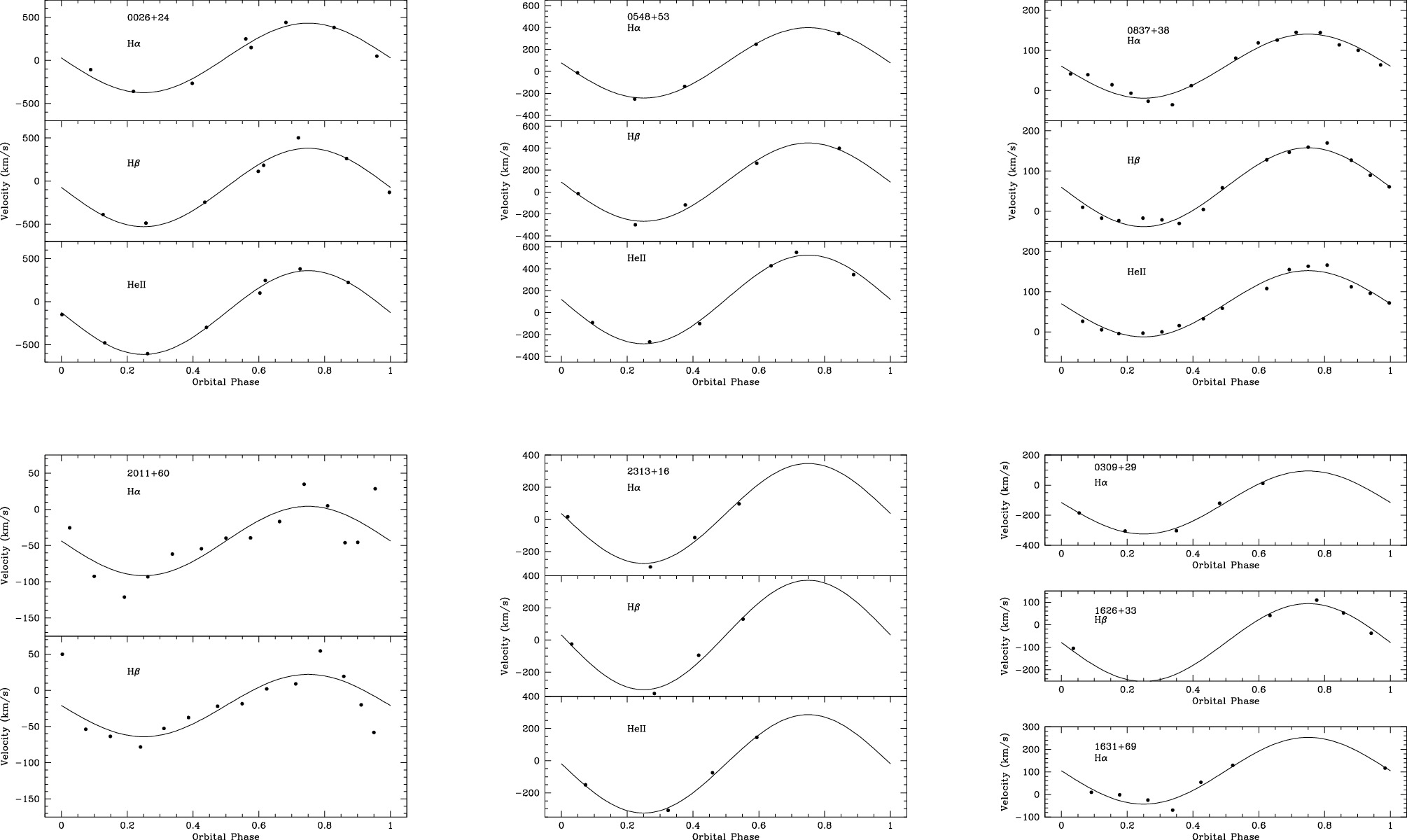
Figure 2. Best-fit sinusoids to the velocities of the objects listed in Table 2.
Download figure:
Standard image High-resolution imageTable 2. Radial Velocity Solutions
| Object | Line | P | γ | K | σ |
|---|---|---|---|---|---|
| (minutes) | (km s−1) | (km s−1) | (km s−1) | ||
| 0026+24 | He ii | 122.9 | −126.2 ± 2.1 | 486 ± 20 | 30 |
| 0026+24 | Hβ | 122.9 | 74.0 ± 4.0 | 455 ± 37 | 62 |
| 0026+24 | Hα | 122.9 | 28.9 ± 3.7 | 403 ± 38 | 58 |
| 0309+29 | Hα | 121.8 | −115.5 ± 5.6 | 210 ± 15 | 13 |
| 0548+53 | He ii | 92.2 | 121.0 ± 1.2 | 405 ± 16 | 24 |
| 0548+53 | Hβ | 92.1 | 90.2 ± 2.5 | 357 ± 21 | 28 |
| 0548+53 | Hα | 92.1 | 77.7 ± 0.8 | 321 ± 7 | 9 |
| 0837+38 | He ii | 190.8 | 69.9 ± 0.3 | 82 ± 4 | 10 |
| 0837+38 | Hβ | 190.8 | 59.7 ± 0.4 | 98 ± 4 | 10 |
| 0837+38 | Hα | 190.8 | 60.9 ± 0.4 | 80 ± 5 | 12 |
| 1626+33 | Hβ | 190.2 | −78.7 ± 17.7 | 172 ± 26 | 14 |
| 1631+69 | Hα | 93.1 | 105 ± 12 | 146 ± 23 | 24 |
| 2011+60 | Hβ | 147.3 | 21 ± 1 | 43 ± 12 | 27 |
| 2011+60 | Hα | 147.3 | 43.7 ± 0.9 | 48 ± 11 | 27 |
| 2313+16 | He ii | 81.6 | −19.6 ± 5.5 | 306 ± 14 | 13 |
| 2313+16 | Hβ | 81.6 | 31 ± 11 | 340 ± 33 | 25 |
| 2313+16 | Hα | 81.6 | 37 ± 8 | 311 ± 25 | 19 |
Download table as: ASCIITypeset image
3.1. 0026+24
The system 0026+24 was discovered as a transient in the CSS survey (Drake et al. 2009) under the identifier CSS 091026:002637+242916. Margon et al. (2014) used the high variability in its light curve obtained with the Palomar Transit Factory, along with follow-up spectra that showed strong Balmer and He ii emission lines to identify this system as containing a magnetic white dwarf. No period was determined for 0026+24. The ZTF light curve (ZTF17aaaehby) shows a range from 17.5 to 20.5 mag (Figure 3). The magnitude at the time of our eight spectra on 2018 December 4 was 18.6, so at a mid-state. The spectrum in Margon et al. (2014) compared to ours (Figure 1) shows a bluer continuum and stronger He ii compared to Hβ than ours, which may be due to a lower level of mass accretion at the time of our spectra. The radial velocities showed periods close to 2 hr for He ii, Hβ, and Hα. A period search using the ZTF light curve revealed an eclipse and refined the period to 2.04760(2) hr (122.9 minutes). Figure 3 shows the power spectrum and light curve folded on this period. The presence of two peaks in the light curve (phases 0.1 and 0.6) is indicative of two accretion poles in view during the orbit. With this fixed period, the final solutions for the velocity curves were obtained and are shown in Table 2 and Figure 2. The large (>400 km s−1) values for the K semi-amplitudes are typical of many polars (see Thorstensen et al. 2020 for a compendium of K velocities for some new polars). The eight spectra shown in Figure 4 are phased according to the spectroscopic phasing, where phase 0 is the red to blue crossing of the velocities. The sequence shows the broad base and narrow component structures that are characteristic of polars, as well as changes in the continuum shape. However, better time-resolved spectra on a larger telescope and polarimetry will be needed to further characterize the system parameters.
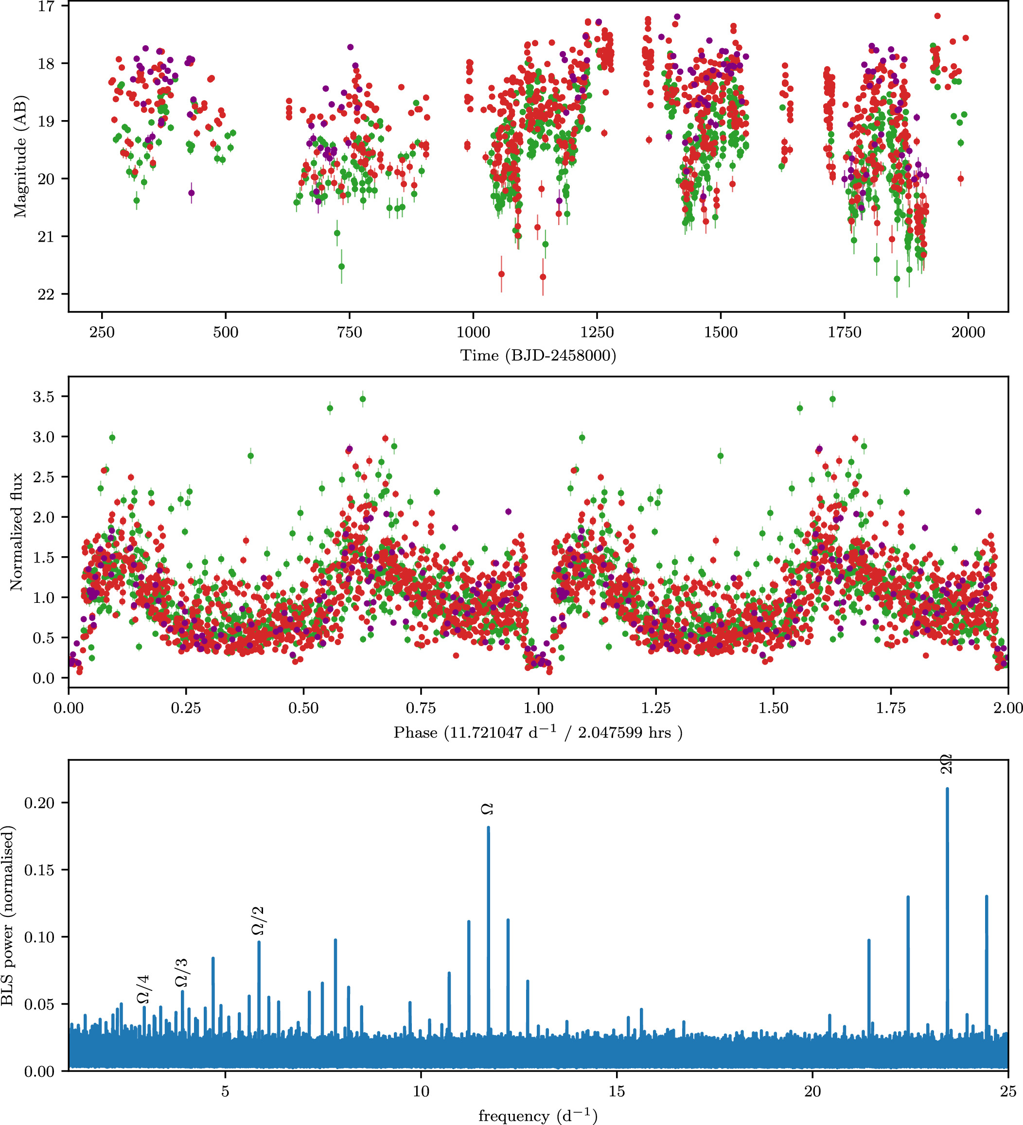
Figure 3. ZTF light curve of 0026+24 (top), data folded on the orbital period showing the presence of an eclipse (middle) and the power spectrum showing the orbital period of 2.05 hr (bottom).
Download figure:
Standard image High-resolution image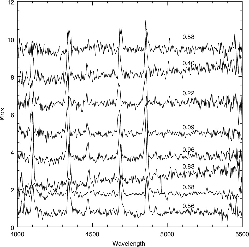
Figure 4. The eight spectra of 0026+24 obtained on 2018 December 4 with the DIS at APO and phased with the spectroscopic phasing.
Download figure:
Standard image High-resolution image3.2. 0309+29
This object was identified as a CV in the CSS (CSS 071108:030945+295251; Drake et al. 2014). Thorstensen et al. (2017) claimed a period of 2.03 hr and the presence of an eclipse. However, no spectrum was shown. The light curves of this object show a range of 15–19, and our spectra were taken at a magnitude of 17, midway between the high and low states. The spectra have low signal-to-noise ratio (S/N), with Hα in emission, but the higher-order Balmer lines have faint emission surrounded by broad absorption and no evidence of helium lines (Figure 1). Our 83 minutes of observation time on 2018 December 4 covers about half an orbit, with the resulting velocity curve for Hα showing a K semi-amplitude of 210 km s−1 (Figure 2, Table 2). There is no evidence for a magnetic nature from these data.
3.3. 0548+53
The American Association of Variable Star Observers (AAVSO) lists this object as MGAB-V330 with an online light curve by G. Murawski and their classification as an eclipsing polar. However, their light curve appears to show high and low states that are typical for a polar, as opposed to eclipses. A light curve from ZTF17aaaheoj is consistent with this interpretation of states (Figure 5). The range in magnitude is 16.5 at a high state and near 20.5 during a low. Gaia shows a mean g magnitude of 19.6 and a parallax of 2.33 ± 0.07 mas, indicating a distance of 429 ± 18 pc. The APO spectra obtained on 2019 April 2 occurred during a high state. One set of blue and red spectra is shown in Figure 1.
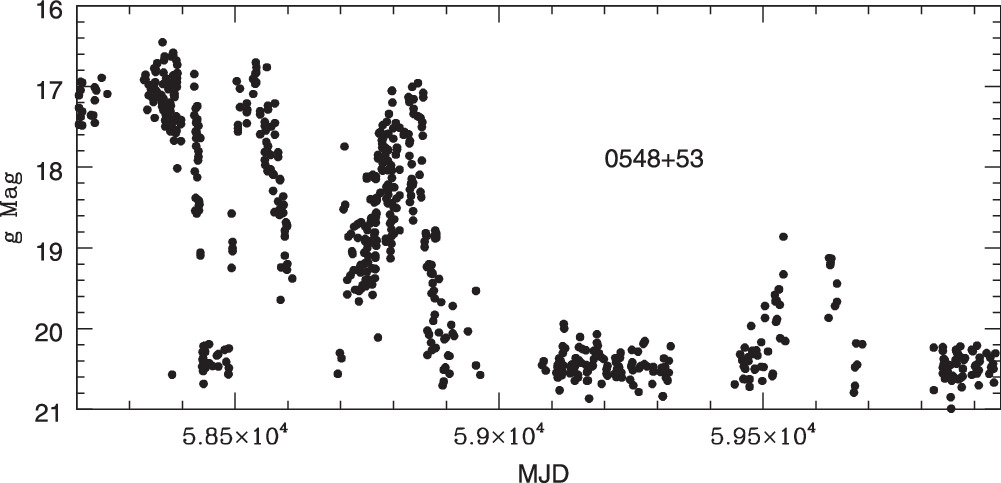
Figure 5. The ZTF light curve of 0548+53 in the g filter, showing the sporadic high and low states that are typical of polars.
Download figure:
Standard image High-resolution imageThe spectra are typical of polars in a high state of accretion, showing Balmer emission lines with narrow components as well as strong He ii lines. Fitting the centroid of the lines to a sine curve produced periods of 89–98 minutes and large K semi-amplitudes near 400 km s−1.
In order to obtain a more precise measurement of the orbital period, we used TESS data (10.17909/wjjd-h183). The source was observed during sector 59 (from 2022 November 26 to 2022 December 23) at a full-frame cadence of 200 s. The power spectrum shows a single peak at 15.627 cycles day−1 (92.1 minutes), which we presume to be the orbital frequency. Fixing the period at this value produces the velocity curve fits shown in Table 2 and Figure 2. The values of period and velocity amplitude are typical of polars.
In addition, broad cyclotron humps that vary in amplitude among the spectra appear near wavelengths of 4300 and 7100 Å (Figure 1). To obtain some estimate of the magnetic field, we used the typical relation between the nth harmonic of the cyclotron and the magnetic field B in megagauss (Ferrario et al. 2015):

where λn is in angstrom and θ is the viewing angle of the cyclotron beaming.
A field strength of 50 MG has the 5th harmonic at 4280 Å and the 3rd harmonic at 7134 Å (the 4th harmonic at 5350 Å is not covered in our spectral range), which is a reasonable fit to our data. Thus, 0548+53 is confirmed as a bona-fide polar.
3.4. 0837+38
This CV (referred to as SDSS J083751.00+383012.5 in the AAVSO Variable Star Index, VSX, catalog) was discovered in the SDSS survey (Szkody et al. 2005), and follow-up photometry, spectroscopy, and spectropolarimetry were reported in Schmidt et al. (2005). Those follow-up observations were all done during a low state that lasted for over 3 yr. Two cyclotron humps were present, indicating a field strength of 65 MG, and the presence of positive and negative polarization showed that both poles were visible during portions of the orbit, and the low amplitudes of variability indicated a low inclination for this system. The power spectrum of the two nights of photometry gave periods of either 3.18 or 3.65 hr, with similar significance, while a fit to a sine wave gave a slightly better fit for the 3.18 hr period.
Our spectra in 2021 were obtained during a high state, with prominent Balmer and He ii emission lines (Figure 1). The velocity fits are given in Table 2 and shown in Figure 2. The best fit for the lines was obtained with a period of 3.18 hr (190.8 minutes), confirming this as the correct period for this system. The fact that it does have high states of accretion shows that this is a regular polar system, not one of the low-accretion-rate polars. The small radial velocity amplitude for a polar could be due to a low inclination to the line-emission area.
3.5. 1626+33
This SDSS discovered object was proposed as a likely polar because of its very strong He ii emission (Szkody et al. 2004). The SDSS spectrum was obtained during a high state. Follow-up spectra obtained in 2015 June (Szkody et al. 2018) had a flux that was about 5 times fainter, with only narrow Balmer emission and little to no ionized helium, indicating a low state. Our five spectra in 2022 May spanned 92 minutes and were similar to the high-state SDSS spectrum.
We searched the ZTF light curve (ZTF18aditqga) for periodic signals. Using the Lomb–Scargle method, we did not find any significant period. However, after detrending the light curve and using a box least-squares method, we did find one significant period, 3.17 hr; see Figure 6. The light curve folded on this period shows a subtle but significant partial eclipse with a depth between 10% and 20%. Using this period, we attempted to fit the radial velocities with the 92 minutes of coverage from the five spectra. The best result was obtained for the Hβ line, with the result listed in Table 2 and shown in Figure 2. Given the limited spectral coverage, further data will be needed to determine the correct identification of system parameters. With the period between 3 and 4 hr, the relatively flat light curve outside the partial eclipse, and the lack of any signal indication of a spin period, it is likely that 1626+33 is a high-accretion-rate SW Sex star, rather than a polar or IP.

Figure 6. The ZTF g-, r-, and i-band light-curve data in green, red, and purple of 1626+33. The top panel shows the unfolded light curve. The middle panel shows the light curve folded on the orbital period after first detrending the data, and shows a subtle but significant eclipse at phase 0. The bottom panel shows the box least-squares power spectrum. We identify the strongest frequency as the orbital frequency (Ω), and also indicate the multiples and significant alias frequencies.
Download figure:
Standard image High-resolution image3.6. 1631+69
As pointed out in Szkody et al. (2020), this system has not been studied in detail, although it was first identified as a CV by Appenzeller et al. (1998). The previous ZTF light curve shown in Szkody et al. (2020) and the recent one (Figure 9) reveal high and low states between 17.5 and 20.5, and spectra taken in 2019 May during a high state showed strong He ii and Balmer emission that changed shape over the course of the hour. Our further spectra obtained in 2021 (57 minutes at APO and 73 minutes at Pal) and in 2023 (148 minutes at APO) also during the high state were similar in appearance to the 2019 data. However, no consistent period could be extracted from the radial velocities alone as large changes in velocity were evident throughout the data sets.
TESS has observed this source extensively, including two separate ∼year-long intervals at the default FFI cadence. Using TESSCut, we downloaded FFI cutouts for 1631+69 in sectors 40, 41, and 47–60 (10.17909/bdjn-y925). The cadence between consecutive points in these light curves was usually 10 minutes, but in the final two sectors it was just 200 s. While TESS data from sectors 14–26 are also available, we ignored them because their 30 minutes cadence is too slow for an analysis of the fast variability in 1631+69.
Although the source was undetected in the data in sectors 56–58, a power spectrum of the remaining sectors reveals the likely orbital and white dwarf spin frequencies as well as their harmonics and sidebands (Figure 7). While the frequency identifications are ambiguous, we believe that the most probable orbital frequency is 15.4682 cycles day−1 (93.1 minutes) based on several circumstantial arguments and reasonable assumptions:
- 1.We assume that the fundamental orbital and spin frequencies are both above the noise in the TESS power spectrum.
- 2.The orbital period is presumed to be above the ∼78 minutes (∼18.5 cycles day−1) period minimum for hydrogen-rich systems.
- 3.We disallow identifications in which a fundamental frequency has a subharmonic. For example, the signal at 20.0 cycles day−1 in Figure 7 cannot be the fundamental spin, orbital, or beat frequency because it is the second harmonic of a frequency at 10.0 cycles day−1.
- 4.We presume that the white dwarf spin frequency is above the binary orbital frequency (as is observed in all well-studied magnetic CVs except for the asynchronous polar V1432 Aql).
- 5.Finally, we expect the frequencies in the power spectrum to generally accord with theoretical predictions and observational results of other IPs.

Figure 7. TESS power spectrum of 1631+69 with frequency identifications expressed as linear combinations of the orbital (Ω), spin (ω), and sampling (fsamp) frequencies.
Download figure:
Standard image High-resolution imageWhile these considerations significantly narrow down the possible frequency identifications, the orbital frequency could be either 15.4682 cycles day−1 or 10.0011 cycles day−1. Fortunately, the absolute Gaia G magnitude of 1631+69 and its GBP − GRP colors can be used to constrain the orbital period of the system, and it is on this basis that we believe that 15.4682 cycles day−1 is the orbital frequency. The Gaia early Data Release 3 distance ( pc; Bailer-Jones et al. 2021), in conjunction with the negligible line-of-sight extinction in the Green et al. (2019) reddening maps and the mean Gaia G magnitude of 20.2, results in an absolute Gaia G magnitude of
  . Abrahams et al. (2022) found that the GBP − GRP color and the absolute G magnitude correlate with the orbital period of a CV, and, based on their Figure 1, G = 11.6 and GBP − GRP = 0.18 are strongly suggestive of an orbital period well below the period gap. The peak at 15.4682 cycles day−1 is the only signal that satisfies both this constraint and our previous requirement that the system have an orbital period above the period minimum.
For an orbital frequency of Ω = 15.4682 cycles day−1, the only plausible identification of the spin frequency is ω = 25.4693 cycles day−1 (56.5 minutes). Assuming that ω > Ω, any other identification of ω would result in subharmonics of either ω or ω − Ω. The resulting spin-to-orbit ratio of 0.607 is anomalously large for an IP, making this system a new member of the rapidly growing class of slowly rotating IPs; see Littlefield et al. (2023, their Figure 5).
Although the McDonald 2.1 m photometry (Figure 8) lacks the year-long baseline of the TESS data, it has superior time resolution and S/N. The 2(ω − Ω), ω, and Ω frequencies in the TESS power spectrum were observed in the McDonald 2.1 m data during 2020 July–September, although the power spectrum varied from night to night. The July 24 data showed the 2(ω − Ω) at 72 minutes, while the August 18 data instead showed two significant periods at 54 and 93 minutes, corresponding with ω and Ω, respectively. Using the precise period from the TESS observations, we are able to derive a long-term ephemeris for the proposed orbital period. Further refinement of the period was accomplished using the McDonald 2.1 m observations, and a zero-point was determined from the dips seen in the light curve in Figure 8, which shows the six nights of McDonald data folded on the adopted (tentative) orbital ephemeris:


Figure 8. McDonald 2.1 m broadband light curves of 1631+69 from 2020 July 24, August 18, September 22, and 2023 May 24 are shown phased with the new orbital ephemeris in the top panels. The sharpest eclipse-like features at cycle 0 (top left) and cycle 15,914 (second row right) were used to establish the orbital ephemeris. The bottom panel shows the photometry folded on the orbital period with the running average superimposed in white.
Download figure:
Standard image High-resolution imageFigure 9 shows the ZTF light curve, power spectrum, and orbital phased data. Because the sampling rate of ZTF is very different than TESS, the power spectrum shows different alias frequencies, but frequencies previously identified as the orbital frequency and spin frequency are both present in the ZTF power spectrum.
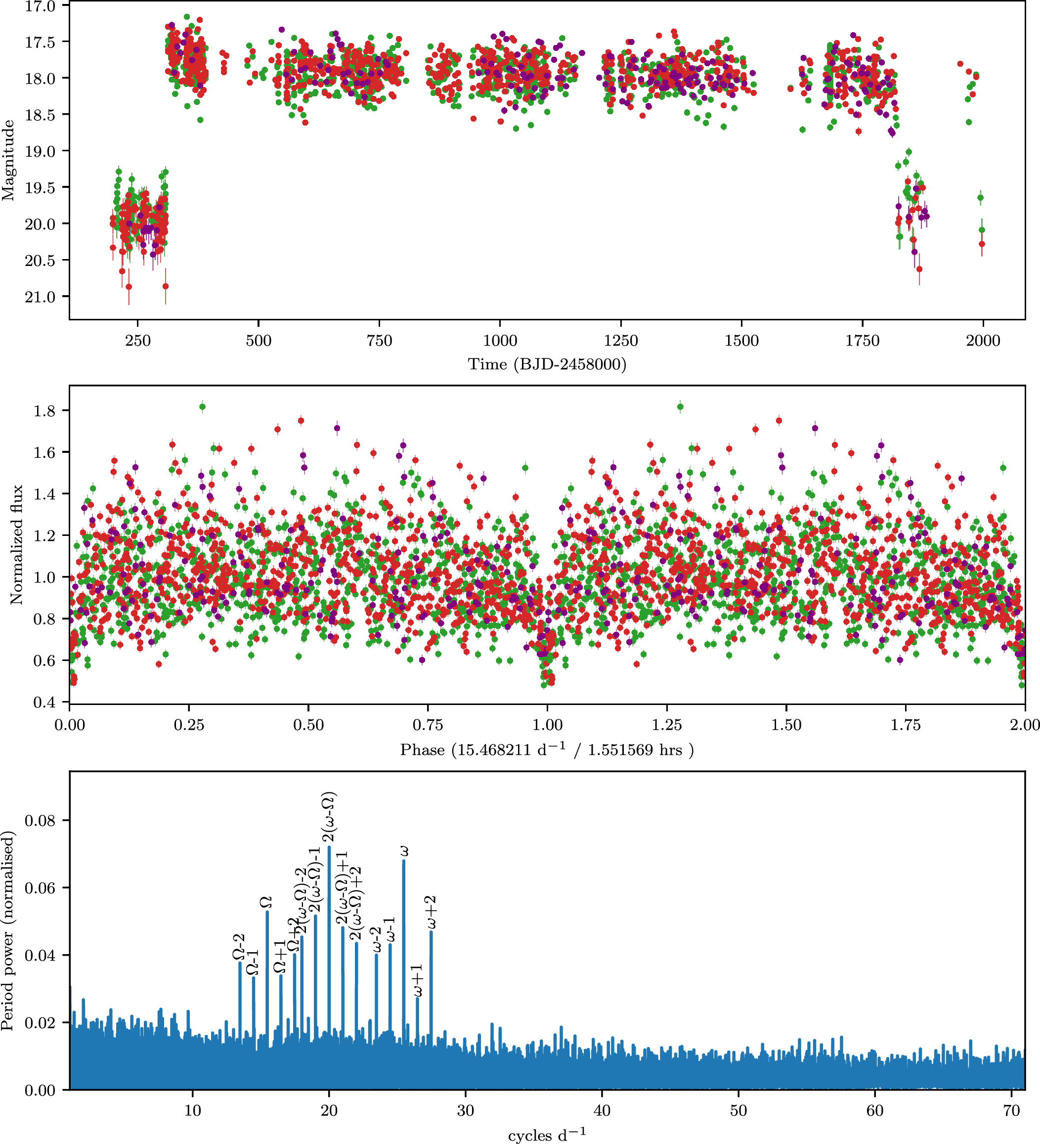
Figure 9. The ZTF g-, r-, and i-band light-curve data in green, red, and purple of 1631+69. The top panel shows the unfolded light curve. The middle panel shows the data folded on the orbital period, with the eclipse at phase 0. The bottom panel shows the Lomb–Scargle power spectrum as calculated from the ZTF high-state data. The orbital frequency and spin frequency are indicated with Ω and ω, the same as in Figure 7.
Download figure:
Standard image High-resolution imageThe McDonald (Figure 8), ZTF (Figure 9), and TESS (Figure 10) data all show a dip in the light curve folded at the orbital frequency Ω, which we identify as a grazing eclipse of the accretion flow. By phase-folding the TESS data, we can disentangle the orbital and beat modulations and glean insight into the highly variable depth of the eclipse in the McDonald data. Figure 10 presents a two-dimensional light curve in which the orbital profile is shown as a function of the system's spin–orbit beat phase. The deepest eclipses occur only at a narrow subset of beat phases.

Figure 10. Two-dimensional TESS light curve of 1631+69, showing the dependence of the orbital profile on the spin–orbit beat phase. Deep eclipses are observed only at certain beat phases, thus explaining the extreme cycle-to-cycle variation in the eclipse depth in the McDonald photometry.
Download figure:
Standard image High-resolution imageReturning to the spectra, even if we force the spectroscopic period to match either of the photometric periods (72 or 93.1), we still cannot produce consistent radial velocity solutions. The best fit occurred for Hα in the 2021 April data (listed in Table 2 and shown in Figure 2). The Hα and Hβ lines from the 2019 data showed comparable values of semi-amplitude (140 ± 43 and 122 ± 24 km s−1, respectively) lending some support to a value near 100 km s−1. However, the longer observation length in 2023 resulted only in a 2–3σ fit with low K amplitudes (43 ± 15 km s−1). It is clear that the K amplitude is not large, even though there is a grazing eclipse. As the emission lines likely arise in the stream/magnetosphere region, it is not so surprising that an orbital modulation is difficult to measure accurately if the inclination is not favorable. The spectra on the night of 2023 May 24 were obtained simultaneously with the McDonald photometry, and included the sharp eclipse at cycle 15994 shown in Figure 8. The eclipse spectrum is fainter and has the reddest velocities for both Hα and Hβ. The spectrum obtained during the brightness peak just after the eclipse has the strongest lines with the continuum only slightly increasing. These results are consistent with an eclipse of a portion of the accretion stream by the secondary as it flows to the white dwarf.
3.7. 2011+60
The variability of this object was detected by both the ATLAS and ZTF sky surveys (Heinze et al. 2018; Ofek et al. 2020). Detailed analysis of the photometry by F. Romanov was published on 2021 February 23 in the AAVSO VSX (Watson et al. 2006) with the name Romanov V48 and later published in Kato & Romanov (2022). No spectra have been published. The photometric data show three periods, identified by Kato & Romanov (2022) as an orbital one at 147.3 minutes, a spin period at 60.62 minutes, and a beat period at 103 minutes. These periods indicated a classification as an IP with a large Pspin/Porb ratio of 0.41. However, an IR excess suggested cyclotron emission and perhaps a polar origin, so the authors suggested this could be an object between an IP and a polar. The long-term ZTF18aawrcla light curve (Figure 11) shows the prominent periods previously identified.
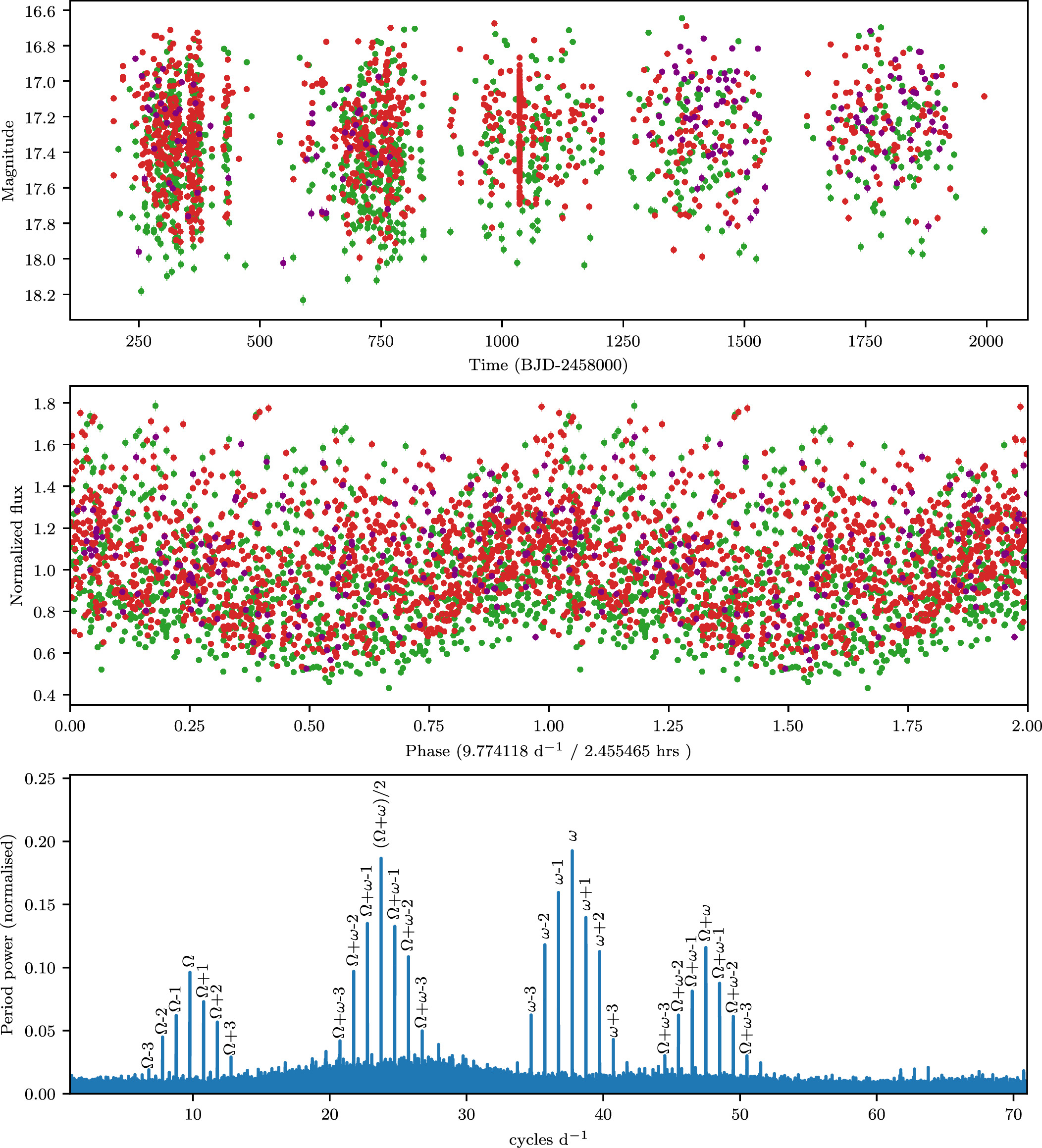
Figure 11. The ZTF g-, r-, and i-band light-curve data in green, red, and purple of 2011+60. The top panel shows the entire light curve. The middle panel shows the data folded on the orbital period. The bottom panel shows the Lomb–Scargle power spectrum showing the orbital (Ω), spin (ω), and combination frequencies.
Download figure:
Standard image High-resolution imageOur spectra from Lick and APO (Figure 1) show the strong He ii indicative of IPs and polars. However, as in 1631+69, the radial velocities of the emission lines showed large scatter (Figure 2), even with fixing the period at 147.3 minutes and the K amplitude of the best fits (Table 2) being not large, indicating a relatively low inclination.
TESS observed 2011+60 in sector 41 (2021 July 23–August 20) and sectors 55–57 (2022 August 5–October 29) at a 2 minutes cadence (10.17909/0yb0-m366). While it was also observed in several earlier sectors, the previous data were obtained at a 30 minutes cadence, so we exclude the older TESS observations from our analysis. A power spectrum of the 2 minutes data shows many periods that are combinations of the spin and orbit periods proposed by Kato & Romanov (2022; see Figure 12).
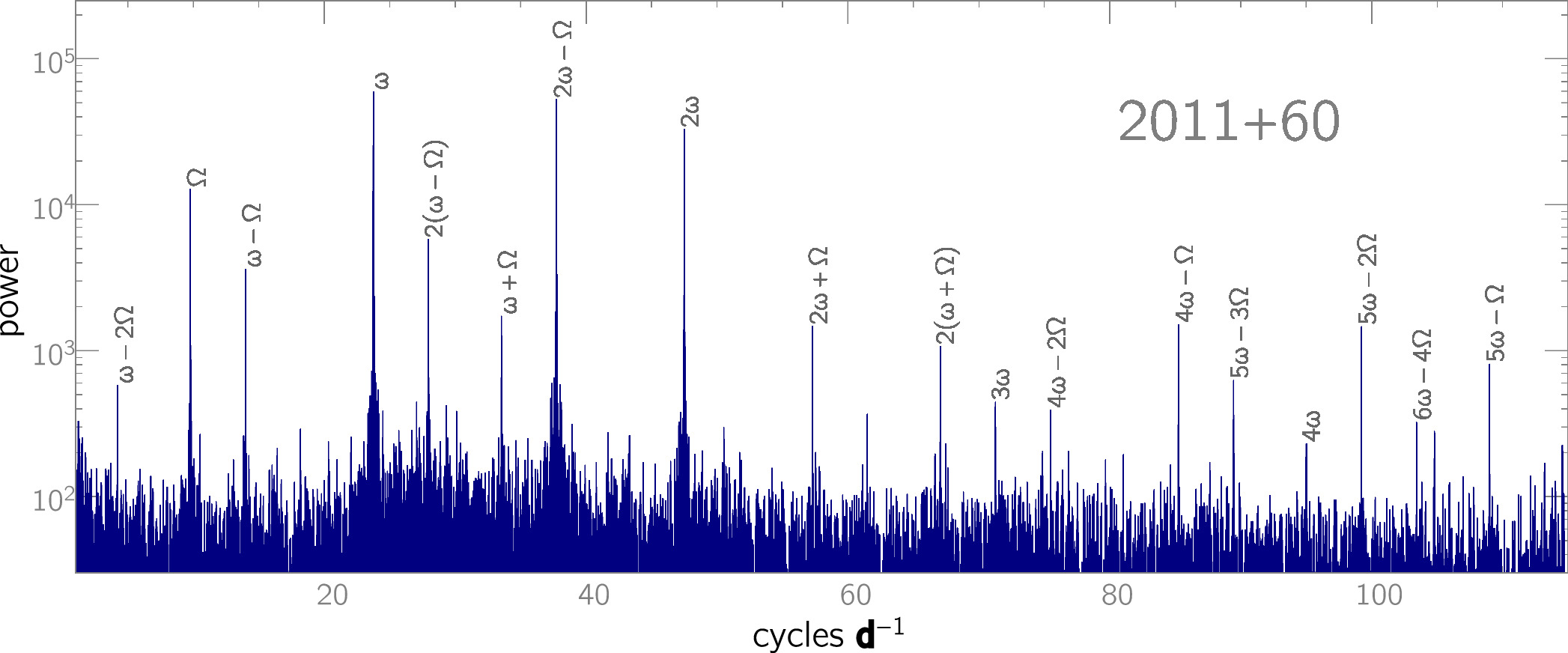
Figure 12. Power spectrum of the TESS data for the diskless IP 2011+60 (Romanov V48), showing the strong orbit (Ω), spin (ω), and beat (ω − Ω) frequencies, as well as their various sidebands and harmonics. The identifications of Ω and ω are identical to those from Kato & Romanov (2022).
Download figure:
Standard image High-resolution imageWe independently arrive at the same frequency identifications proposed by Kato & Romanov (2022). Using the Abrahams et al. (2022) method to predict the orbital period from the Gaia absolute G magnitude and GBP − GRP colors, we would expect the orbital period to be ∼3 hr, and only one signal in the observed power spectrum matches this prediction: the 9.77 cycles day−1 (147.3 minutes) frequency identified by Kato & Romanov (2022) as the orbital frequency. Additionally, the Kato & Romanov (2022) identification of the spin period is significantly more reasonable than other choices; for example, if the 2ω − Ω signal in Figure 12 were actually the true spin frequency ω, the resulting beat frequency ω − Ω would have a subharmonic, which is implausible with a Lomb–Scargle spectrum. While we believe the Kato & Romanov (2022) frequency identifications to be correct, they nonetheless require confirmation of their origins, as with 1631+69.
Notably, the likely orbital period at 147.3 minutes places 2011+60 in the period gap; with the solitary exception of Paloma, all IPs with large Pspin/Porb ratios are below the period gap (Figure 5 in Littlefield et al. 2023).
When the spin period is phased with the beat cycle (Figure 13), large changes in the spin profile are evident, as first noted by Kato & Romanov (2022) from their analysis of the ZTF data. The TESS data show this effect in more detail.
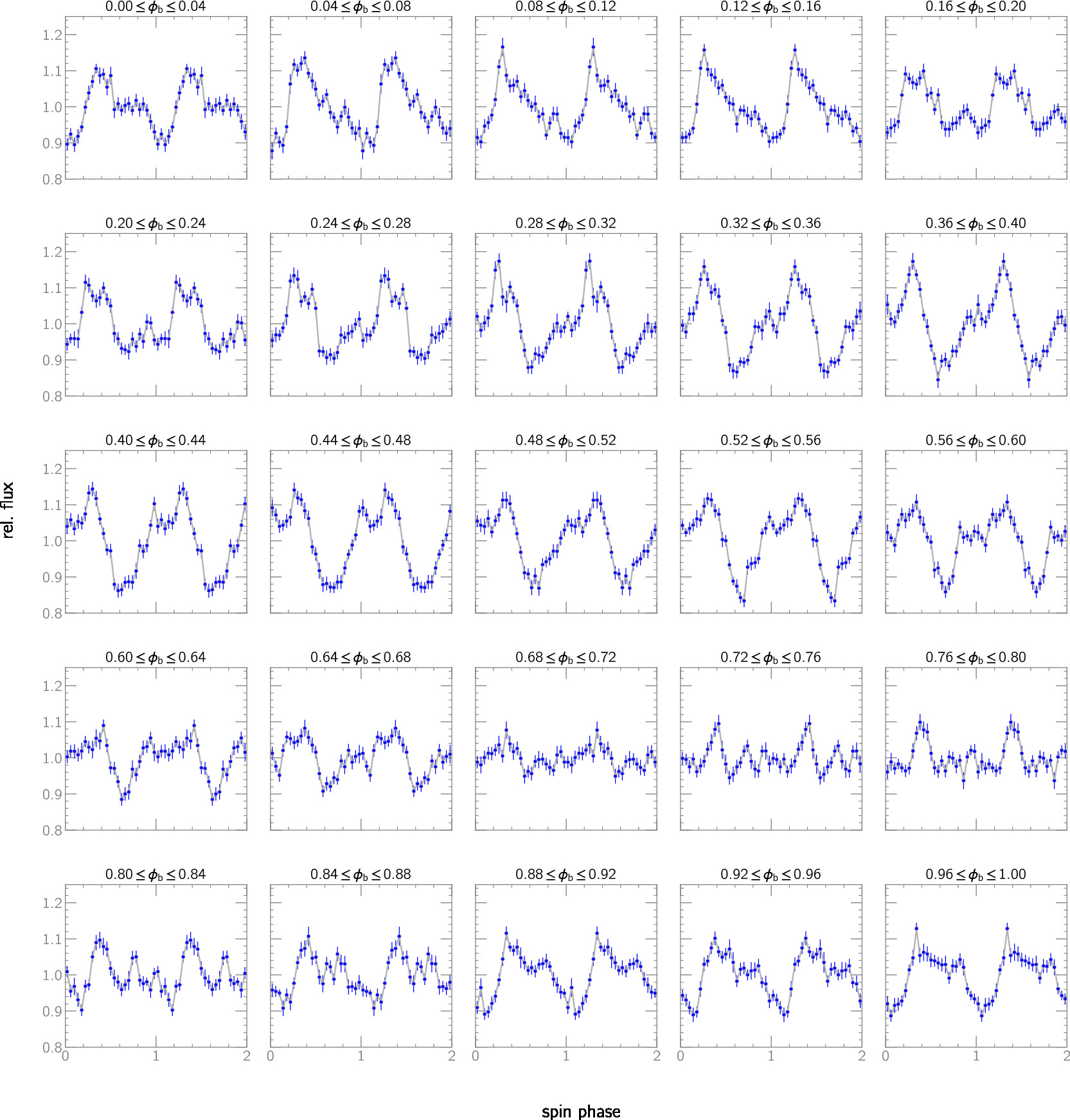
Figure 13. TESS data of 2011+60 (Romanov V48), folded on the spin and beat periods, showing the large changes in the spin profile during the beat phase. Phase 0 is arbitrary.
Download figure:
Standard image High-resolution imageWhile a disk-fed IP would show a more uniform spin modulation of the two accretion curtains, Figure 13 shows some evidence of the two poles (beat phases 0.88–0.04), whereas at other times (beat phases 0.08–0.16, 0.28–0.40), there are sharp peaks present in the pole visible at spin phase 0.3. This likely means that there is some input from the mass-transfer stream to the magnetosphere.
These data all confirm 2011+60 being a short-period member of the IP class.
3.8. 2313+16
Margon et al. (2014) identified 2313+16 as a potential magnetic CV based on its spectrum showing strong He ii emission and the PTF light curve that revealed a period of 1.36 hr (81.6 minutes). We were only able to obtain four spectra, but they cover 0.52 of its orbit so we were able to construct a radial velocity curve (Figure 2). The results shown in Table 2 reveal a high K semi-amplitude that is typical of polars, as well as large changes in the He ii strength during the 53 minutes of observations. This lends support to a classification of 2313+16 as a polar, while the skewed appearance of the light curve both in Margon et al. (2014) and in our ZTF folded light curve (Figure 14) is more typical of an IP. Our spectrum shown in Figure 1 is fairly similar to that shown in Margon et al. (2014), although the continuum shape is different, with less blue light in the APO spectrum. However, the Margon et al. (2014) spectrum was normalized so it is difficult to do a direct comparison, and the phase coverage may also be different.
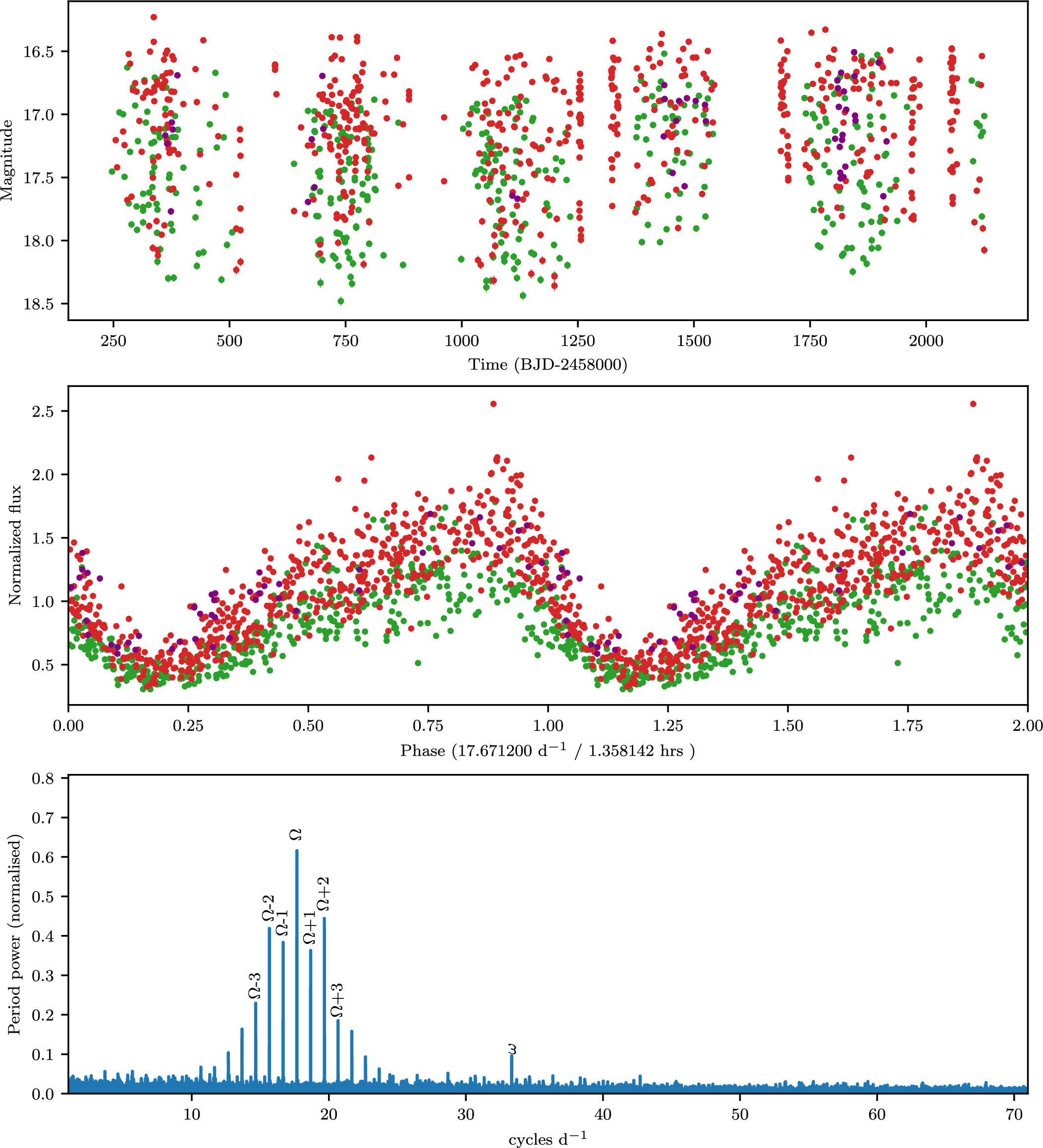
Figure 14. The ZTF g-, r-, and i-band light-curve data in green, red, and purple of 2313+16. The top panel shows the entire light curve. The middle panel shows the data folded on the orbital period. The bottom panel shows the Lomb–Scargle power spectrum showing the orbital (Ω) and possible spin frequencies (ω), including alias frequencies.
Download figure:
Standard image High-resolution imageIn analyzing the ZTF data, we clearly recovered the orbital period (Figure 14). We also detected a significant peak in the power spectrum at 33.3 day−1 (43.19 minutes), which we originally thought could be a spin frequency. It is 1.9 times the orbital frequency and therefore not a harmonic of the orbital period. However, the TESS power spectrum of 2313+16, which was obtained 2022 September 1–30 from 200 s of cadence FFI data in sector 56 (10.17909/g2jp-6m34), shows only orbital harmonics, with no evidence of the 33.3 day−1 signal (Figure 15). The most likely explanation for this is that the 33.3 day−1 signal in the ZTF data is an alias of the second harmonic of the orbital frequency, as it is exactly 2 day−1 below that harmonic.
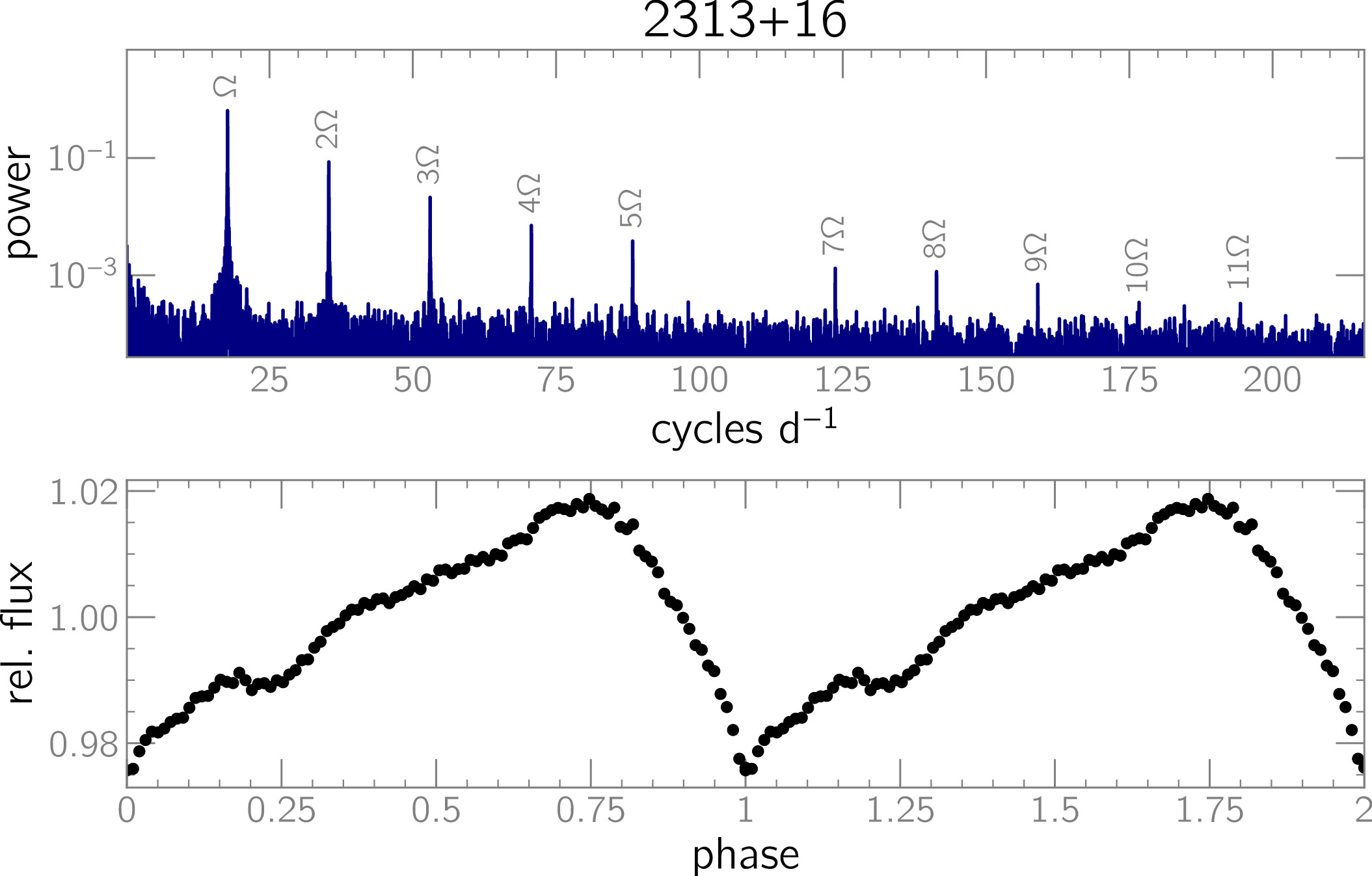
Figure 15. TESS power spectrum and phased light curve of 2313+16. The power spectrum shows no evidence of the 33.3 day−1 signal in the ZTF data, while the phased TESS light curve shows a shallow, well-defined dip. Phase 0 was defined arbitrarily to coincide with this dip, but without a radial velocity curve of the secondary it is unknown whether this dip coincides with the secondary's inferior conjunction. Because 2313+16 has significant blending, the true amplitude of variation is much larger than it is in TESS.
Download figure:
Standard image High-resolution image
The folded TESS data (Figure 15) show a sharp dip that may be indicative of a partial eclipse, as well as a broader dip a quarter of a phase later that could be caused by a stream or the effects of a second pole. Polarimety would be very helpful to clarify the correct classification of this object.
4. Conclusions
Spectroscopic observations on CVs potentially harboring highly magnetic white dwarfs are a useful tool in confirming the correct classification and physical characteristics of these systems, especially when accompanied by available TESS, ZTF, good-time-resolved ground-based photometry, and Gaia distances. Our study of eight systems provides the following detailed information that will be useful in studies of CV populations and close binary evolution.
- 1.The ZTF light curve of 0026+24 reveals an orbital period of 122.9 minutes and a total eclipse, while spectra show a high radial velocity amplitude and broad and narrow emission-line components. The light curve shows two maxima, which would be consistent with two accretion poles in view. This object is very likely a polar.
- 2.0309+29 shows no evidence of a magnetic nature.
- 3.TESS data on 0548+53 reveals an orbital period of 92.1 minutes, while high-state spectra show a high K amplitude, emission lines with narrow and broad components, and broad cyclotron features indicating a magnetic field strength of 50 MG. This object is thus confirmed as a polar.
- 4.High-state spectra of 0837+38 resolve the ambiguity in orbital period from previous low-state photometry, revealing the correct period to be 190.8 minutes.
- 5.Analysis of the ZTF light curve of 1626+33 resulted in the discovery of a partial eclipse and a period of 3.17 hr. The long period, together with the lack of any spin period, indicates this object could be a high-accretion-rate SW Sex system.
- 6.Using extensive TESS data, an orbital period of 93.1 minutes as well as a spin period of 56.5 minutes was found, making 1631+69 a new member of the class of slowly rotating IPs. The ZTF data independently confirm these periods. McDonald photometry, as well as the ZTF and TESS data folded on the orbital period, all show a grazing eclipse, while the TESS orbital data plotted as a function of the spin–orbit beat phase shows the deepest eclipses occur only at a narrow subset of the beat phases. While radial velocities show large scatter, the data are consistent with much of the emission originating in the stream flow.
- 7.Power spectra of the ZTF and TESS observations of 2011+60 confirm the orbital, spin, and beat periods proposed by Kato & Romanov (2022), as well as revealing many combinations of the spin and orbit. The TESS high-time-resolution data over extended days show the detailed changes that occur in the spin profile during the beat cycle. The radial velocities show large scatter with low K amplitude.
- 8.The radial velocities of 2313+16 show a large K semi-amplitude typical of polars, while the ZTF light curve is more similar to an IP, showing a skewed sine curve. The power spectrum of the ZTF data reveals both the orbital period of 81.6 minutes found by Margon et al. (2014) as well as a significant signal at 43.19 minutes, but TESS data show only the orbital period, so the shorter period may be due to an alias of the second harmonic of the orbital period. The folded TESS data show features that may be indicative of partial eclipses of a stream or poles. Further polarimetric data will be needed to determine the correct nature of this object.
Acknowledgments
J.v.R. was supported from NWO grant No. VI.Veni.212.201. Based on observations obtained with the Samuel Oschin Telescope 48 inch and the 60 inch Telescope at the Palomar Observatory as part of the Zwicky Transient Facility project. ZTF is supported by the National Science Foundation under grant Nos. AST-1440341 and AST-2034437 and a collaboration including current partners Caltech, IPAC, the Weizmann Institute of Science, the Oskar Klein Center at Stockholm University, the University of Maryland, Deutsches Elektronen-Synchrotron and Humboldt University, the TANGO Consortium of Taiwan, the University of Wisconsin at Milwaukee, Trinity College Dublin, Lawrence Livermore National Laboratories, IN2P3, University of Warwick, Ruhr University Bochum, Northwestern University and former partners the University of Washington, Los Alamos National Laboratories, and Lawrence Berkeley National Laboratories. Operations are conducted by COO, IPAC, and UW. The Gordon and Betty Moore Foundation, through both the Data-Driven Investigator Program and a dedicated grant, provided critical funding for SkyPortal. Also based on observations obtained with the Apache Point Observatory 3.5 m telescope, which is owned and operated by the Astrophysical Research Consortium and at the McDonald Observatory 2.1 m telescope owned and operated by the University of Texas. The latter observations were funded by Picture Rocks Observatory. This paper includes data collected with the TESS mission, obtained from the MAST data archive at the Space Telescope Science Institute (STScI). Funding for the TESS mission is provided by the NASA Explorer Program. STScI is operated by the Association of Universities for Research in Astronomy, Inc., under NASA contract NAS 5-26555.