


1. Introduction
Understanding the interactions of polymer molecules and hydrodynamic flows are among the most fundamental topics in the interdisciplinary research areas of fluid mechanics, chemical engineering and polymer physics (Lumley Reference Lumley1969; Bird Reference Bird1987). When subjected to various flow conditions, polymer molecule may exhibit rich behaviours of morphing chain configurations as revealed by single molecule visualization techniques (Perkins, Smith & Chu Reference Perkins, Smith and Chu1997; Smith, Babcock & Chu Reference Smith, Babcock and Chu1999), leading to intriguing bulk rheological and physical properties (Fuller & Leal Reference Fuller and Leal1980; Menasveta & Hoagland Reference Menasveta and Hoagland1991; Hunkeler, Nguyen & Kausch Reference Hunkeler, Nguyen and Kausch1996; Lee et al. Reference Lee, Dylla-Spears, Teclemariam and Muller2007). Of particular interest is the study of the coil-stretch (C-S) transition of long-chain macromolecules, such as DNAs, in flows of dilute solutions. When the background flow has a non-zero velocity gradient (e.g. shear and elongational flows), at certain critical conditions, the coiled polymers can abruptly unwind to become elongated or fully stretched shapes due to the imposed fluid viscous force, termed as the C-S transition (Smith & Chu Reference Smith and Chu1998). More interestingly, when measuring the polymer's end-to-end distance as a function of the extension rate, the transition typically features hysteresis behaviours, suggesting a bistable system with more than one equilibrium state.
In the early 1970s, DeGennes (Reference DeGennes1974) introduced the initial kinetic model of an elastic dumbbell to predict the hysteresis behaviours observed in elongational flows during the C-S transition. He attributed these phenomena to the shape-dependent viscous force acting on the polymer chain. As the DNA unfolds, the initially hidden monomers become more exposed to hydrodynamic flows. By not explicitly considering fluid–polymer interactions, de Gennes demonstrated that the hysteresis behaviours can be effectively described by a double-well potential, which combines the effects of the background elongational flow and the elastic forces in the dumbbell spring. The same mechanism was pointed out independently by Hinch (Reference Hinch1974, Reference Hinch1977) and was supported by several other authors (Tanner Reference Tanner1975; Fuller & Leal Reference Fuller and Leal1981). Instead of using phenomenological double-well potentials, they resolved the hysteresis using similar elastic dumbbell models that incorporated length-dependent hydrodynamic friction forces. Apart from the hydrodynamic effects, all these models emphasized the importance of employing nonlinear elastic constitutive laws to account for the finite extensibility of polymer chains (Peterlin Reference Peterlin1961; Larson Reference Larson1988). Further investigation into various microscopic aspects of the C-S transition, involving calibrating the effective conformational energy (Schroeder, Shaqfeh & Chu Reference Schroeder, Shaqfeh and Chu2004), determining the threshold of molecular weight (Hsieh & Larson Reference Hsieh and Larson2005) and studying the characteristic post-extension relaxation time (Doyle et al. Reference Doyle, Shaqfeh, McKinley and Spiegelberg1998) and ergodicity-breaking mechanisms in model reduction (i.e. from polymer chain to dumbbell, Beck & Shaqfeh Reference Beck and Shaqfeh2007), were extensively explored using Brownian dynamics simulations based on beads-spring-chain models, which accounted for bead–bead hydrodynamic interactions.
In a broader context, abrupt configurational transitions have often been observed in microfluidic systems where various thin elastic structures of much larger sizes than polymer molecules interact with strong viscous flows. For example, a fluid vesicle (Kantsler, Segre & Steinberg Reference Kantsler, Segre and Steinberg2008; Narsimhan, Spann & Shaqfeh Reference Narsimhan, Spann and Shaqfeh2015; Kumar, Richter & Schroeder Reference Kumar, Richter and Schroeder2020) under extension can exhibit sharp transitions from tubular to dumbbell shapes. More interestingly, a thin elastic sheet of different shapes in elongational flows may undergo a ‘compact-stretched’ transition with hysteresis, akin to the C-S transition of polymer molecules (Silmore, Strano & Swan Reference Silmore, Strano and Swan2021; Yu & Graham Reference Yu and Graham2021, Reference Yu and Graham2022). As demonstrated by Yu & Graham (Reference Yu and Graham2021, Reference Yu and Graham2022), who performed direct simulation of flexible sheets in flows, successfully achieving C-S transition at the macro scale requires the use of finite-extensibility elastic models, such as the Yeoh elastic model (Yeoh Reference Yeoh1993). The intriguing aspect of cross-scale observations of C-S transitions is that they indicate the existence of specific universal hydrodynamic coupling mechanisms for a class of problems involving interactions between fluids and elastic structures. These mechanisms are applicable to small polymer molecules but are independent of the stochastic nature of the microsystem. In fact, Hinch (Reference Hinch1974, Reference Hinch1977) previously suggested the possibility of connecting the chain unfolding process to the stretching deformation of a homogeneous ellipsoidal elastic particle (EP), a reduced-order mechanical model for dilute, coiled polymers and was initially introduced by Cerf (Reference Cerf1952) and later extended by Roscoe (Reference Roscoe1967). Compared with stochastic kinetic models for elastic dumbbells or bead-spring chains, the EP model is mathematically simpler and has much fewer degrees of freedom, and naturally captures the shape-dependent hydrodynamic effects that become increasingly dominant in strong flows. But the EP model cannot represent polymer chains since it oversimplifies the intricate heterogenous coiled microstructures, and ignores the stochastic features such as Brownian forces.
Although the early models (Cerf Reference Cerf1952; Goddard & Miller Reference Goddard and Miller1967; Roscoe Reference Roscoe1967) successfully accounted for shape-dependent fluid forces, their simple elastic constitutive laws (e.g. linear or neo-Hookean elastic model) fail to describe the constitutive relation at high strains, making them incapable of capturing hysteresis phenomena. Recognizing this limitation, the natural progression, as also suggested by Hinch (Reference Hinch1977), is to incorporate different nonlinear constitutive laws to mimic polymer chain's finite extensibility in strong flows. Continuing along this line of investigation, in this study we present an improved EP model to investigate the C-S transition of polymer molecules. Despite having been proposed several decades ago, the precise mathematical formulation of the EP model incorporating finite extensibility has yet to be thoroughly examined. Here we employ an analytical approach originally derived by the author (Gao, Hu & Ponte Castañeda Reference Gao, Hu and Ponte Castañeda2011, Reference Gao, Hu and Ponte Castañeda2012, Reference Gao, Hu and Ponte Castañeda2013) to describe EP deformation. The method utilizes the polarization technique (Eshelby Reference Eshelby1957, Reference Eshelby1959; Willis Reference Willis1981) to derive an exact solution for the isolated nonlinear EP problem under simple Stokes flow conditions (i.e. flows with constant velocity gradients). To account for finite and large deformation behaviours, we employ the incompressible Gent hyperelastic model (Gent Reference Gent1996; Avazmohammadi & Ponte Castañeda Reference Avazmohammadi and Ponte Castañeda2015), which captures significant strain hardening at large strains. As demonstrated below, this new model unveils the elastohydrodynamics of the C-S transition in uniaxial elongational flows, regulated by finite extensibility, and robustly captures hysteresis phenomena that are akin to polymer chain behaviours. It is worth emphasizing that the Gent model was chosen primarily due to its simple two-parameter form, facilitating analytical manipulations. We have also tested other similar strain-hardening models, such as the Yeoh model (Yeoh Reference Yeoh1993), which qualitatively captures similar transition behaviours. Additionally, we can explain the system's bistability through a free-body diagram at steady state without relying on dynamic properties (e.g. relaxation time) of polymer chains. Furthermore, the model allows for convenient extraction of other analytical features, such as the sharpness of the transition region, and enables systematic examination of their dependencies on material and geometric parameters, including stiffness, flow rate and initial shapes.
The structure of the paper is outlined as follows. In § 2 we provide a concise overview of the polarization method based on Eshelby's solution and derive the condition for the steady-state deformation of a Gent EP under uniaxial extension. Section 3 focuses on examining the characteristic steady-state solutions and unveiling the C-S transition phenomenon by monitoring the principal stretch of the semi-major axis of the spheroid as the flow strength increases. Moreover, we elucidate the physical mechanisms behind the observed hysteresis behaviours through force-balance analysis. In addition, we have also investigated the use of alternative constitutive laws, such as the Yeoh hyperelastic model, which accounts for the strain-hardening effect, and observed similar C-S transition behaviours. Finally, some conclusions are drawn in § 4.
2. Mathematical model
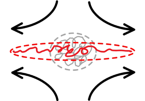
Our study focuses on investigating the dynamics of a long-chain polymer that is initially coiled and exposed to an unbounded, uniaxial three-dimensional elongational flow  $( \dot {\gamma } x_1, -({\dot {\gamma }}/{2}) x_2, -({\dot {\gamma }}/{2}) x_3)$ with constant flow rate
  $\dot {\gamma }$. In our approach, rather than explicitly modelling the intricate details of the flexible chains, we approximate the polymer as an isotropic, incompressible EP. This particle is assumed to possess an ellipsoidal shape that instantaneously adjusts to the flow conditions and exhibits a no-slip surface, as depicted in figure 1. In the limit of a vanishingly small Reynolds number (
 $Re\rightarrow 0$), the continuity and momentum equations can be expressed in a coherent manner throughout the entire domain as
 \begin{equation} \boldsymbol{\nabla}\boldsymbol{\cdot} {{\boldsymbol{v}}} = 0\quad {\rm and} \quad \boldsymbol{\nabla} \boldsymbol{\cdot} {\boldsymbol{\sigma}} = \textbf{0}. \end{equation}
In the Eulerian fluid domain  $\varOmega _f$ (denoted by subscript ‘
 $f$’), the total stress tensor
  $\boldsymbol {\sigma }_f$ is defined by the constitutive relation
 \begin{equation} \boldsymbol{\sigma} _f ={-} p_f {{\boldsymbol{I}}} + 2 \mu {{\boldsymbol{D}}}_f, \end{equation}
where  $\mu$ is the fluid viscosity,
  $p_f$ is the pressure and
  ${{\boldsymbol{D}}}_f = \frac {1}{2}( {\boldsymbol {\nabla }{{\boldsymbol{v}}} + {\boldsymbol {\nabla } {{\boldsymbol{v}}} }^{\rm T}})$ is the rate-of-deformation or strain-rate tensor. Likewise, in the solid particle domain
  $\varOmega _s$ (denoted by the subscript ‘
 $s$’), we define
 \begin{equation} \boldsymbol{\sigma}_s={-} p_s{{\boldsymbol{I}}} + \boldsymbol{\tau}, \end{equation}
where  $p_s$ is a pseudo-pressure, serving as a Lagrangian multiplier to enforce the incompressibility constraint. In general, the extra solid stress
  $\boldsymbol {\tau }$ can be defined as a function of the Finger (or left Cauchy–Green) tensor
  ${{\boldsymbol{B}}} = {{\boldsymbol{F}}} {{\boldsymbol{F}}}^T$, with
  ${{\boldsymbol{F}}} ={{\partial {{\boldsymbol{x}}}}}/{{\partial {{\boldsymbol{X}}}}}$ denoting the deformation gradient tensor, where
  $\{{{\boldsymbol{x}}}\}$ and
  $\{{{\boldsymbol{X}}}\}$ denote the current and reference domain, respectively. For a neo-Hookean solid with the shear modulus
  $\eta$, the extra stress is taken as
  $\boldsymbol {\tau } = \eta ({{\boldsymbol{B}}} -{{\boldsymbol{I}}})$, which permits infinite strain. For the purpose of modelling solids with finite extensibility, we have opted to utilize the incompressible Gent model whose constitutive relation can be written as
 \begin{equation} {{\boldsymbol{\tau }}} = {\eta } {{{\left( {1 - \frac{{I_1 - 3}}{J}} \right)}^{ - 1}}\left( {{\boldsymbol{B}}} - {{\boldsymbol{I}}} \right)} = {\eta } \chi \left( {{\boldsymbol{B}}} - {{\boldsymbol{I}}} \right), \end{equation}
which is derived from an elastic potential energy  $W = -({\eta J}/{2}) \ln (1 - ({I_1 - 3)}/{J})$ (Gent Reference Gent1996; Avazmohammadi & Ponte Castañeda Reference Avazmohammadi and Ponte Castañeda2015). Notably, the prefactor
  $\chi = {{( {1 - ({{I_1 - 3}})/{J}} )}^{ - 1}}$ in the equation signifies the finite extensibility of the polymer chain, where
  $I_1$ is the so-called first invariant of the Cauchy strain tensor. Besides
  $\eta$, the only new parameter, the strain limit constant
  $J>0$, determines the maximum allowable values for the principal stretches. It is evident that the elastic stress
  ${{\boldsymbol {\tau }}}$ will become unbounded as
  $I_1$ approaches the upper limit of
  $J+3$, effectively capturing the strain-hardening behaviour. When
  $J \rightarrow \infty$ is chosen, the Gent model automatically recovers the neo-Hookean model without enforcing stiffening at large strain. The rate of change of
  ${\boldsymbol{B}}$ satisfies the evolution equation (Joseph Reference Joseph1990)
 \begin{equation} \frac{{\rm D}{{\boldsymbol{B}}}}{{\rm D}t} = {\boldsymbol{\nabla} {{\boldsymbol{v}}} }^T \boldsymbol{\cdot} {{\boldsymbol{B}}} + {{\boldsymbol{B}}}\boldsymbol{\cdot} {\boldsymbol{\nabla} {{\boldsymbol{v}}} }, \end{equation}
where  ${{{\rm D}{}}/{{\rm D}t}}= {\partial }/{\partial t} + ({{\boldsymbol{v}}} \boldsymbol {\cdot }\boldsymbol {\nabla })$ denotes a material time derivative. The set of governing equations (2.1a,b)–(2.5), along with the velocity and traction continuity conditions at the fluid–solid interface, will be simultaneously solved. To non-dimensionalize the above equations, we have chosen the characteristic length scale as the particle size
  $d_p$, the time scale
  $\dot {\gamma }^{-1}$, the velocity scale
  $\dot {\gamma } d_p$ and the pressure and stress scale
  $\mu \dot {\gamma }$. The elastic deformation is characterized by the shear modulus
  $\eta$. Hence, the dimensionless parameter defined as
  $G={\mu \dot {\gamma }}/{\eta }$ measures the viscous force in the fluid relative to the elastic force in the solid, and hence, can be termed as an effective ‘stretching’ parameter that characterizes the magnitude of the elastic stretching deformation subjected to the elongational flow field.

Figure 1. Schematic of the EP model for C-S transition of an initially coiled long-chain polymer. The spheroidal envelop with the semi-axes  $a_0 \geqslant b_0 = c_0$ will deform axisymmetrically into a more slender shape at the steady state.
The polarization method developed by Gao et al. (Reference Gao, Hu and Ponte Castañeda2011), derived from the classical Eshelby problem in composite materials (Eshelby Reference Eshelby1957, Reference Eshelby1959), offers additional analytical tools for manipulating the aforementioned fluid–solid system. This method leverages the insight that a uniform (yet potentially time-dependent) strain rate and vorticity fields within the particle indicate that the particle undergoes a series of transformations into ellipsoidal shapes before reaching a final steady state (Goddard & Miller Reference Goddard and Miller1967; Roscoe Reference Roscoe1967; Bilby, Eshelby & Kundu Reference Bilby, Eshelby and Kundu1975; Bilby & Kolbuszewski Reference Bilby and Kolbuszewski1977; Hinch Reference Hinch1977; Ogden Reference Ogden1984; Wetzel & Tucker Reference Wetzel and Tucker2001). The key step is introducing a uniform, incompressible ‘reference’ medium for the solid phase with the same viscosity  $\mu _f$ as the fluid phase, and define the dimensionless stress polarization tensor
  $\boldsymbol {\varXi }$ as the total stress difference, or ‘polarization tensor’
 \begin{equation} {\boldsymbol{\varXi }} = {\boldsymbol{\sigma }} + p {{\boldsymbol{I}}}- 2{{\boldsymbol{D}}}. \end{equation}
Here we have dropped the subscripts ‘f’ and ‘s’ in the definition so that the governing equations can be universally constructed in the entire domain as
 \begin{equation} \boldsymbol{\nabla}\boldsymbol{\cdot} {{\boldsymbol{v}}} = 0,\quad \nabla ^2 {{\boldsymbol{v}}} -\boldsymbol{\nabla} p + \boldsymbol{\nabla}\boldsymbol{\cdot} {\boldsymbol{\varXi }}= \textbf{0}, \end{equation}
which can be reinterpreted as an equivalent problem for the homogeneous reference medium subjected to a distribution of body force  $\boldsymbol {\nabla }\boldsymbol {\cdot }{\boldsymbol {\varXi }}$ in the particle. Hence, the solution of the velocity field
  ${\boldsymbol{v}}$ of the forced Stokes equation in (2.7a,b) can be represented as
 \begin{equation} {\boldsymbol{v}} \left( {{\boldsymbol{x}}} \right) ={\boldsymbol{L}}^0 \boldsymbol{\cdot} {\boldsymbol{x}}+ \int_{\varOmega_s} {\boldsymbol{G}}^{0}({{\boldsymbol{x}}},{{\boldsymbol{x}}'}) \boldsymbol{\cdot} (\boldsymbol{\nabla}_{{\boldsymbol{x}}'} \boldsymbol{\cdot} {\boldsymbol{\varXi }}) {\rm d}{{\boldsymbol{x}}'}, \end{equation}
where the volume integral is performed over the solid domain  $\varOmega _s$,
  ${\boldsymbol{L}}^0$ represents the imposed far-field velocity gradient and
  ${\boldsymbol{G}}^{0}({{\boldsymbol{x}}},{{\boldsymbol{x}}'})$ is the free-space Green's function or Stokeslet. By rewriting the tensor
  ${\boldsymbol{G}}^{0}$ in the Fourier space and applying on the uniform forcing field, the strain-rate tensor
  ${{\boldsymbol{D}}}_s = \frac {1}{2}( {\boldsymbol {\nabla } {{\boldsymbol{v}}} + {\boldsymbol {\nabla } {{\boldsymbol{v}}} } ^{\rm T}})$ and the vorticity tensor
  ${{\boldsymbol{W}}}_s = \frac {1}{2}( {\boldsymbol {\nabla } {{\boldsymbol{v}}} - {\boldsymbol {\nabla } {{\boldsymbol{v}}} }^{\rm T}})$ are found to be given by
 $$\begin{gather} {{\boldsymbol{D}}}_s = \left( {\mathbb{I} - 2\mathbb{P} } \right)^{ - 1}: ({{{\boldsymbol{D}}}^0 - \mathbb{P}:{\boldsymbol{\tau}}}), \end{gather}$$
 $$\begin{gather}{{\boldsymbol{W}}}_s = {{\boldsymbol{W}}}^0 - \mathbb{R} : {\boldsymbol{\tau}} + 2\mathbb{R} \boldsymbol{\cdot} ({( {\mathbb{I} - 2\mathbb{P}})^{ - 1}: ({{{\boldsymbol{D}}}^0 - \mathbb{P}: {\boldsymbol{\tau}}})}). \end{gather}$$
In the above,  $\mathbb {I}$ is the fourth-order identity tensor,
  $\mathbb {P}$ and
  $\mathbb {R}$ (see results for spheroidal particles in Appendix A) are two fourth-order tensors related to the instantaneous shape of the particle,
  ${{\boldsymbol{D}}}^0 = \frac {1}{2}({\boldsymbol{L}}^0 + ({\boldsymbol{L}}^0)^{\rm T})$ and
  ${{\boldsymbol{W}}}^0 = \frac {1}{2}({\boldsymbol{L}}^0 - ({\boldsymbol{L}}^0)^{\rm T})$ are the background strain-rate and vorticity tensors. The readers are referred to more derivation details in Gao et al. (Reference Gao, Hu and Ponte Castañeda2011). It should be pointed out that our definition of the shape tensors is different from the classical Eshelby tensors in solid mechanics literature (Eshelby Reference Eshelby1957, Reference Eshelby1959; Wetzel & Tucker Reference Wetzel and Tucker2001, see also Willis (Reference Willis1981) and Ponte Castañeda (Reference Ponte Castañeda2005) for more discussion on these choices). Another direct implication of this is that all the spatial gradients on the stress (or strain) fields in the equations, such as the convective term in (2.5), vanishes automatically. With (2.9) and (2.9), the original coupled partial differential equations now convert to a systems of ordinary differential equations for solving the time-dependent (uniform) solid stress and particle shape regarding the aspect ratios and orientation.
In a uniaxial extensional flow, we consider an EP that initially possesses a spheroidal shape (with  $a_0 \geqslant b_0 = c_0$), and the semi-major axis is aligned with the
  $x$ axis. When subjected to uniaxial fluid loading, the EP will deform axisymmetrically into another thinner spheroidal shape (
 $a > b = c$) with the aspect ratio
  $\omega = b/a = c/a$. Thus, in the limit case of a spherical particle shape, denoted as
  $\omega = 1$, it represents a polymer in a perfectly coiled state. Conversely, as
  $\omega$ approaches 0, it corresponds to a fully stretched polymer. The principal stretches of elastic deformation can be written as
 \begin{equation}
{\lambda _1} = {\Bigl(
{\frac{\omega}{{{\omega_0}}}} \Bigr)^{ - 2/3}},\quad
{\lambda _2} = {\lambda _3} = {\Bigl(
{\frac{\omega}{{{\omega_0}}}}\Bigr)^{1/3}} ,
\end{equation}
\begin{equation}
{\lambda _1} = {\Bigl(
{\frac{\omega}{{{\omega_0}}}} \Bigr)^{ - 2/3}},\quad
{\lambda _2} = {\lambda _3} = {\Bigl(
{\frac{\omega}{{{\omega_0}}}}\Bigr)^{1/3}} ,
\end{equation}
where  $\omega _0 = b_0/a_0$ is the initial aspect ratio. Following the definition in (2.4), together with the condition of volume incompressibility of an EP (i.e.
  $a_0 b_0 c_0 = a b c$, or
  $a_0 b_0^2 = a b^2$ for a spheroid), it is straightforward to obtain the expressions for the three stress components as
 \begin{gather} \tau _{11} =
\frac{\chi}{G}({{\lambda^2 _1} - 1}) = \frac{1}{G}{\Bigl(
{1 - \frac{{{I_1} - 3}}{J}} \Bigr)^{ - 1}}\Bigl({{{\Bigl(
{\frac{\omega }{\omega_0 }} \Bigr)}^{ - 4/3}} - 1}
\Bigr),
\end{gather}
\begin{gather} \tau _{11} =
\frac{\chi}{G}({{\lambda^2 _1} - 1}) = \frac{1}{G}{\Bigl(
{1 - \frac{{{I_1} - 3}}{J}} \Bigr)^{ - 1}}\Bigl({{{\Bigl(
{\frac{\omega }{\omega_0 }} \Bigr)}^{ - 4/3}} - 1}
\Bigr),
\end{gather} \begin{gather}\tau _{22} = \tau _{33} =
\frac{\chi}{G}( {{\lambda^2_{2}} - 1} ) =
\frac{1}{G}{\Bigl( {1 - \frac{{{I_1} - 3}}{J}} \Bigl)^{ -
1}}\Bigl( {{{\Bigl( {\frac{\omega }{\omega_0 }}
\Bigr)}^{2/3}} - 1} \Bigr).
\end{gather}
\begin{gather}\tau _{22} = \tau _{33} =
\frac{\chi}{G}( {{\lambda^2_{2}} - 1} ) =
\frac{1}{G}{\Bigl( {1 - \frac{{{I_1} - 3}}{J}} \Bigl)^{ -
1}}\Bigl( {{{\Bigl( {\frac{\omega }{\omega_0 }}
\Bigr)}^{2/3}} - 1} \Bigr).
\end{gather}
Here it is important to highlight that utilizing the principal strain  ${\lambda _i}$ defined in (2.11a,b) to evaluate the first invariant
  $I_1$ in (2.4) is inaccurate. On the one hand, the geometric constraint defined in the prefactor
  $\chi$ entails setting a limit on the maximum attainable length of a fully extended chain, and this limit should not depend on the initial aspect ratio
  $\omega _0$. On the other hand, the unconstrained part of (2.4), i.e. the Hookean stress–strain relation, requires using the strain that is defined based on the initial configurations that may become partially unfolded already (i.e.
  $\omega _0> 0$). Thus, when determining the value of
  $I_1$ in
  $\chi$, we opt to consistently compare the deformed shape to that of a spherical shape, i.e. fixing
  $\omega _0 = 1$ for a perfectly coiled shape, and evaluate
  $I_1$ using a set of ‘reference’ principal strain (denoted by superscript ‘
 $(r)$’) as
 \begin{equation} I_1 = I^{(r)}_1 = \sum_{i = 1}^3 {(\lambda^{(r)} _i)^2} = {\omega}^{ - 4/3}({1 + 2{\omega}^2}), \end{equation}
with
 \begin{equation} {\lambda^{(r)} _1} = {\omega}^{ - 2/3},\quad {\lambda^{(r)} _2} = {\lambda^{(r)} _3} = {{\omega}^{1/3}}. \end{equation}
Since the particle will not rotate during the symmetric extension, i.e.  ${{\boldsymbol{W}}}_s = \textbf {0}$ automatically satisfied, the steady-state solution only requires
 \begin{equation} {{\boldsymbol{D}}}_s = \textbf{0} \end{equation}
in (2.9).
3. Results and discussion
Applying the imposed background strain-rate tensor  ${\boldsymbol{D}}^0 = {\rm {diag}}\{1, -1/2, -1/2\}$ and the stress components in (2.16), after some algebraic manipulations, we are able to solve the stretching parameter
  $G$ as a function of the steady-state aspect ratio
  $\omega = \varOmega$ as
 \begin{equation} G = \frac{{{J}(
{{\varOmega ^2} - {\omega_0 ^2}})\biggl( {\left(
{\dfrac{{{\varOmega ^2} + 2}}{{\sqrt {1 - {\varOmega ^2}}
}}} \right)\ln \Bigg( {\dfrac{{1 - \sqrt {1 - {\varOmega
^2}} }}{{1 + \sqrt {1 - {\varOmega ^2}} }}} \Bigg) + 6}
\biggr)}}{{4 {\omega_0 ^{2/3}}{{( {1 - {\varOmega ^2}})}^2}[{\left( {{J} + 3} \right) {\varOmega ^{ -
2/3}} - 2 - {\varOmega ^{ - 2}}}]}}.
\end{equation}
\begin{equation} G = \frac{{{J}(
{{\varOmega ^2} - {\omega_0 ^2}})\biggl( {\left(
{\dfrac{{{\varOmega ^2} + 2}}{{\sqrt {1 - {\varOmega ^2}}
}}} \right)\ln \Bigg( {\dfrac{{1 - \sqrt {1 - {\varOmega
^2}} }}{{1 + \sqrt {1 - {\varOmega ^2}} }}} \Bigg) + 6}
\biggr)}}{{4 {\omega_0 ^{2/3}}{{( {1 - {\varOmega ^2}})}^2}[{\left( {{J} + 3} \right) {\varOmega ^{ -
2/3}} - 2 - {\varOmega ^{ - 2}}}]}}.
\end{equation}
(Or, equivalently, we can numerically solve  $\varOmega$ as a function of
  $G$.) In the limit of
  $J \rightarrow \infty$, the above equation reduces to the neo-Hookean case where
 \begin{equation} G = \frac{{(
{{\varOmega ^2} - {\omega_0 ^2}})\biggl( {\left(
{\dfrac{{{\varOmega ^2} + 2}}{{\sqrt {1 - {\varOmega ^2}}
}}} \right)\ln \Bigg( {\dfrac{{1 - \sqrt {1 - {\varOmega
^2}} }}{{1 + \sqrt {1 - {\varOmega ^2}} }}} \Bigg) + 6}
\biggr)}}{{4{(\omega_0/\varOmega)
^{2/3}}{{({1 - {\varOmega ^2}})}^2}}}.
\end{equation}
\begin{equation} G = \frac{{(
{{\varOmega ^2} - {\omega_0 ^2}})\biggl( {\left(
{\dfrac{{{\varOmega ^2} + 2}}{{\sqrt {1 - {\varOmega ^2}}
}}} \right)\ln \Bigg( {\dfrac{{1 - \sqrt {1 - {\varOmega
^2}} }}{{1 + \sqrt {1 - {\varOmega ^2}} }}} \Bigg) + 6}
\biggr)}}{{4{(\omega_0/\varOmega)
^{2/3}}{{({1 - {\varOmega ^2}})}^2}}}.
\end{equation}
Subsequent analyses and discussions will rely on these fundamental solutions as the basis for further examination. As shown in figures 2(a)–2(c), the hysteretic C-S transition behaviours are captured when plotting the steady-state value of the principal stretch (i.e. square root of the principal strain) along the semi-major axis against  $G$, corresponding to the scenarios of changing the effective particle stiffness (or, increasing the flow strength). Here we examine two types of strain measurements, namely the actual strain
  ${\varLambda } = {( {{\varOmega }/{{{\omega _0}}}} )^{ - 2/3}}$ in (2.11a,b) and the reference strain
  ${\varLambda }^{(r)} = {{\varOmega }^{ - 2/3}}$ defined in (2.15a,b). The discrepancy lies in the fact that
  ${\varLambda }$ quantifies the deformation relative to the initial state, which can possess different shapes (i.e.
  $0 < \omega _0 \leqslant 1$), whereas
  ${\varLambda }^{(r)}$ exclusively measures the deformation relative to a reference spherical shape (i.e. fixing
  $\omega _0 = 1$). Consequently, the maximum value of
  ${\varLambda }^{(r)}$ effectively signifies the finite length of a fully stretched polymer, and is independent of the initial state.

Figure 2. Principal stretch of the semi-major axis as a function of stiffness  $G$ for (a) an initially spherical particle
  $\omega _0 = 1$ with different values of
  $J$, and (b,c) an initially spheroidal particle when choosing
  $0<\omega _0\leqslant 1$ and fixing
  $J = 1000$. In panels (a,b) the dashed line recovers the neo-Hookean model that was previously obtained by Gao et al. (Reference Gao, Hu and Ponte Castañeda2011) and Roscoe (Reference Roscoe1967). The principal stretch is measured with respect to the actual initial shape (
 $\varLambda$ in panel b) and with respect to the reference spherical shape (
 $\varLambda ^{(r)}$ in panel c). In panel (c) the inset shows the zoom-in view in the vicinity of
  $G = 0$.
For both types of strain definitions, we can identify two branches of solutions, respectively marked as the ‘C’ and ‘S’ state. The S solution branch characterizes the strain-hardening effect, i.e. producing larger elastic deformation to counterbalance the increasing fluid extensional force, which is obviously missing in the neo-Hookean model. In panel (a) we fix the initial shape to be spherical so that  ${\varLambda } = {\varLambda }^{(r)}$, and vary the strain limit value
  $J$. The C-S transition exhibits a relatively smooth and nearly monotonic behaviour for small values of
  $J$. However, as
  $J$ surpasses approximately 300, the transition becomes sudden and exhibits hysteresis. As
  $J$ continues to increase towards infinity, the C-S transition progressively diminishes due to the Gent model converging towards the neo-Hookean model. This trend is illustrated by the black dashed line, which corresponds to the previous results obtained by Roscoe (Reference Roscoe1967) and Gao et al. (Reference Gao, Hu and Ponte Castañeda2013). In panel (b) we fix
  $J = 1000$ and examine the initial shape effect by varying
  $\omega _0$. As anticipated, initiating the process from a more elongated shape or a pre-stretched configuration leads to an earlier occurrence of the C-S transition, particularly at lower values of
  $G$. Moreover, the transition demonstrates a sharper progression towards a fully stretched configuration, which is consistent with experimental observations for DNAs (Smith & Chu Reference Smith and Chu1998). If the initial spheroidal shape is already considerably thin, only an S branch is present (illustrated by the green curve computed at
  $\omega _0 = 0.05$), indicating an immediate transition to a fully stretched shape. Moreover, the dashed lines representing the neo-Hookean cases for non-spherical shapes consistently demonstrate a single C state without any transition. In panel (c) we analyse the measurement of the reference strain
  $\varLambda ^{(r)}$ for the same cases as presented in panel (b). The inset on the left provides a zoom-in visual representation of the EP undergoing deformation from various initial shapes, or ‘stressless’ configurations, characterized by different values of
  $\varLambda ^{(r)}$ at
  $G = 0$. All S curves are seen to saturate at the maximum allowable strain
  $\varLambda _{max}$ which, by definition, can be obtained by directly solving the geometric constraint
 \begin{equation} \varLambda^2_{max} + \frac{2}{\varLambda_{max}} = J + 3, \end{equation}
suggesting that the chain eventually unfolds to the same maximum length set by  $J$ (Horgan Reference Horgan2015).
Next, we seek a more quantitative characterization of the hysteresis regime during the transition. As shown by the inset of figure 3(a), the extent of the hysteresis region in figure 2 can be determined by measuring the two turning points on the  $\varLambda - G$ curves, namely
  $G_{min}$ and
  $G_{max}$, which are obtained by solving the roots of equation
 \begin{equation} {\left. {\frac{{{\rm d}G}}{{{\rm d}\varOmega }}} \right|_{\varOmega = {\varOmega _c}}} = 0 \end{equation}
from (3.1). In panel (a) we plot  $G_{max}$ and
  $G_{min}$ as functions of the initial aspect ratio
  $\omega _0$ at different values of
  $J$. Evidently, the hysteresis region generally appears narrower at lower values of
  $\omega _0$ and
  $J$, indicating a more abrupt transition. (The zoomed-in view within the inset highlights a particularly rapid transition at
  $J = 400$.) On the contrary, as the value of
  $J$ increases, the transition region expands gradually, whereby the upper limit
  $G_{max}$ approaches the neo-Hookean case, and the lower limit
  $G_{min}$ decreases. Another intriguing observation is that for initially spherical shapes at
  $\omega _0=1$, a consistent value of
  $G_{max}\approx 0.34$ is maintained across all large and finite values of
  $J$ (
$J$ ( $J>300$) when two turning points are present, and hence, serves as a global maximum. This result even aligns with the findings for initially circular elastic sheets undergoing C-S transition in elongational flows using the Yeoh hyperelastic model (Yu & Graham Reference Yu and Graham2021). In panel (b) we plot the steady-state aspect ratio
  $\varOmega _c = \varOmega _{min}$ and
  $\varOmega _c = \varOmega _{max}$ that corresponds to
  $G_{max}$ and
  $G_{min}$, respectively. With increasing
  $J$, the upper limit tends to converge towards the neo-Hookean case, whereas the lower limit diminishes to zero. In panel (c) we gather data for the ‘thinnest’ initial shape, represented by
  $\omega _0 = \omega ^{*}_0$, as a function of
  $J$ that can induce hysteresis. Mathematically, these instances correspond to the stationary reflection points on the
  $\varLambda - G$ curves, resulting in the merging of the two bounds in panel (b), denoted as
  $\varOmega _c = \varOmega _{min} = \varOmega _{max}$. For all the cases considered, we identify a global minimum
  $J_{min} \approx 330$ as
  $\omega _0^{*} \rightarrow 1$ for initially spherical EPs.

Figure 3. Phase diagrams for computational parameters to characterize hysteresis. (a) The width of the hysteretic regime featured by the distance between the turning points of the  $G - \varLambda$ curves. The upper (
 $G_{max}$, marked by solid lines) and lower (
 $G_{min}$, marked by dashed lines) bounds as a function of initial aspect ratio
  $\omega _0$ at some typical values of
  $J$. (b) The corresponding values of
  $\varOmega _{min}$ (for
  $G_{max}$) and
  $\varOmega _{max}$ (for
  $G_{min}$) as functions of
  $\omega _0$. (c) The minimum initial aspect ratio
  $\omega _0^{*}$ for hysteresis to occur as a function of
  $J$.
$J$.
To understand the underlying mechanism behind the hysteresis behaviour captured by the EP model, we employ the analysis approach introduced by Gao et al. (Reference Gao, Hu and Ponte Castañeda2013) to examine the force balance of the half-spheroid, as depicted in figure 4. When subjected to a simple uniaxial elongation field, the deformation of the EP is primarily governed by the interplay between external hydrodynamic forces and internal elastic resistance forces along the  $x$ axis. We utilized the fundamental solutions for a rigid ellipsoidal particle moving in Stokes flows derived by Jeffery (Reference Jeffery1922) to calculate the horizontal fluid extensional force exerted on the particle surface
  $\partial S_h$ as
 \begin{equation} F_{fluid} = \oint_{\partial S_h} {\hat{\boldsymbol{e}}_1}\boldsymbol{\cdot} (\boldsymbol{\sigma}_f\boldsymbol{\cdot} \boldsymbol{n}){\rm d}S, \end{equation}
where  $\hat {\boldsymbol {e}}_1$ is the unit vector along the
  $x$ axis. The external fluid force is counterbalanced by the internal elastic force exerted upon the middle cross-section of the particle. Since the stress and strain fields in the particle are uniform, the responsive force
  $F_{elastic}$ can be then simply expressed as
 \begin{equation} F_{elastic} = (\boldsymbol{\sigma}_s \boldsymbol{\cdot} {\hat{\boldsymbol{e}}_1}) \times A , \end{equation}
where  $A = {\rm \pi}b^2$ is the surface area. It is important to note a subtle point in our analysis. We choose to evaluate the deviatoric component of the fluid stress, denoted as
  $\boldsymbol {\sigma }_f = 2{{\boldsymbol{D}}}_f$, and incorporate the pressure difference between the two phases into the solid stress, denoted as
  $\boldsymbol {\sigma }_s = -(p_s - p_f){\boldsymbol{I}} + {{\boldsymbol {\tau }}}$. This choice allows us to eliminate the arbitrary reference pressure. Furthermore, this approach has the advantage of making the fluid force
  $F_{fluid}$ solely dependent on the shape of the EP, while the elastic force
  $F_{elastic}$ is influenced by various factors including the EP's shape, stiffness and strain limit.

Figure 4. Force balance of the half-spheroidal EP revealing the physical mechanism of hysteresis. Both the Gent (solid lines) and the neo-Hookean (dashed lines) models are tested for initially spherical EP, i.e.  $\omega _0 = 1$ for some typical values of
  $G$. Inset: free-body diagram of the half-spheroid. The filled and open symbols mark the stable and unstable equilibrium states, respectively.
Theoretically,  $F_{fluid}$ and
  $F_{elastic}$ must balance in steady states. As depicted in figure 4, where we keep the initial shape
  $\omega _0 = 1$ and strain limit
  $J = 1000$, hysteresis can be observed based on the phase diagrams shown in figure 3. The steady-state solutions are obtained by determining the intersections of the two functions,
  $F_{fluid}(\varOmega )$ (represented by the black solid line) and
  $F_{elastic}(\varOmega, G)$. The number of intersections directly indicates the characteristic properties of the C-S transition. When choosing a small
  $G$ (e.g.
  $G = 0.2$ marked as a green line), there is only one intersection, corresponding to the solutions on the C branch of the
  $\varLambda - G$ curves in figure 2. Similarly, for a large value of
  $G$ (e.g.
  $G = 0.5$ indicated by the blue line), the presence of a single intersection corresponds to the S branch of the transition. Nevertheless, if we select a value of
  $G$ within the transition regime defined by
  $G \in [G_{min}, G_{max}]$ as shown in figure 3, we can observe three intersections along the red line. From left to right, these intersections are labelled as states 1, 2 and 3 in figure 4. Let us focus on state 1 located on the C branch. If
  $\varOmega$ decreases (increases) slightly from the intersection point (i.e. the particle becomes slightly more elongated),
  $F_{elastic}$ becomes larger (smaller) than
  $F_{fluid}$, causing the EP to contract (stretch) correspondingly to restore the equilibrium configuration. The same conceptual analysis applies to state 3 on the S branch. Therefore, both of these equilibrium solutions are stable and indicated by filled circles. In contrast, applying the same analysis to state 2 represented by an open circle reveals an opposite trend. When
  $\varOmega$ slightly decreases (increases),
  $F_{elastic}$ becomes smaller (larger) than
  $F_{fluid}$, causing the EP to continue extensional (contracting) without reaching equilibrium. At this point, a numerical linear stability analysis could be employed to characterize the system behaviour quantitatively and more rigorously. However, we find that the bistability analysis described above, although simplistic, is intuitive and straightforward. It also aligns with the earlier kinetic models (DeGennes Reference DeGennes1974; Hinch Reference Hinch1974, Reference Hinch1977; Fuller & Leal Reference Fuller and Leal1980), and reflects the essence of the phenomenological double-well potential. As comparisons, we investigate the corresponding cases under the neo-Hookean model, seen as the dashed lines. As anticipated, no bistable solutions are observed, and only a stable C branch exists. Additionally, we have identified a second class of equilibrium solutions, referred to as state 4 and denoted by the open diamond, during the transition. However, just like state 2, it is evident that these solutions are determined to be unstable.
Finally, we conduct an additional verification to confirm the validity of the physical mechanisms identified above. Instead of utilizing the Gent model, we employ the Yeoh model (Yeoh Reference Yeoh1993), which is another widely used nonlinear hyperelastic model that incorporates strain hardening. The incompressible Yeoh model is characterized by a constitutive relation with a three-parameter form
 \begin{gather} \tau _{11} =
\frac{1}{G}{( {1 + z_1(I_1 - 3)+
z_2(I_1 - 3)^2})}\Bigl({{{\Bigl(
{\frac{\omega }{\omega_0 }} \Bigr)}^{ - 4/3}} - 1}
\Bigr), \end{gather}
\begin{gather} \tau _{11} =
\frac{1}{G}{( {1 + z_1(I_1 - 3)+
z_2(I_1 - 3)^2})}\Bigl({{{\Bigl(
{\frac{\omega }{\omega_0 }} \Bigr)}^{ - 4/3}} - 1}
\Bigr), \end{gather}
 \begin{gather}
\tau _{22} = \tau _{33} =\frac{1}{G}{( {1 + z_1(I_1 - 3)+
z_2(I_1 - 3)^2})}\Bigl( {{{\Bigl(
{\frac{\omega }{\omega_0 }} \Bigr)}^{2/3}} - 1} \Bigr),
\end{gather}
\begin{gather}
\tau _{22} = \tau _{33} =\frac{1}{G}{( {1 + z_1(I_1 - 3)+
z_2(I_1 - 3)^2})}\Bigl( {{{\Bigl(
{\frac{\omega }{\omega_0 }} \Bigr)}^{2/3}} - 1} \Bigr),
\end{gather}
with  $z_{1,2}$ the material constants (
 $z_{1,2} = 0$ reduces to the neo-Hookean model). As shown in figure 5, when selecting suitable values for the parameters
  $z_{1,2}$ in the Yeoh model, an EP governed by the Yeoh model demonstrates hysteresis in the C-S transition when measuring the principal stretch, which bears qualitative similarities to the hysteresis observed in a Gent EP. It is noteworthy that the Yeoh model, which does not impose a restriction on the maximum strain, exhibits generally smoother stiffening behaviours at high strains. In panel (b) we demonstrate that by simultaneously adjusting two parameters, more versatile control over the stiffening behaviours at high strains can be achieved compared with using a single-parameter form in (2.12) and (2.13). The impact of the initial shape is investigated in panel (c), where similar trends to the Gent model are observed, i.e. the transition becomes sharper for thinner shapes and the global maximum
  $G_{max} \approx 0.34$ when choosing
  $\omega _0 = 1$. A closer examination in panel (d) reveals that the equilibrium solutions on the lower C branch, including the turning points for different
  $\omega _0$, are nearly independent of the specific model used. This is because all these nonlinear models accurately capture small and finite elastic deformations. Consequently, the simple neo-Hookean model should accurately predict the C states, while the S states may exhibit some variations when different models are employed.

Figure 5. Principal stretch of the semi-major axis as a function of stiffness  $G$ for the Yeoh model (Yeoh Reference Yeoh1993). (a) Initially spherical particle
  $\omega _0 = 1$ at
  $z_1 = 0$ and different values of
  $z_2$. (b) Initially spherical particle
  $\omega _0 = 1$ at different values of
  $z_1$ while fixing
  $z_2 = 10^{-7}.$ (c) Spheroidal particle with different
  $\omega _0$ and fixing
  $z_1 = 0$ and
  $z_2 = 10^{-7}$. (d) Zoom-in view of the ‘C’ branch for both the Yeoh (solid lines) and Gent (dotted lines,
  $J = 1000$) models.
4. Conclusion
We have presented an EP model with finite extensibility to restudy the C-S transition of dilute polymers under steady elongational flows. Unlike previous kinetic models that were developed for weak flows with ad-hoc hydrodynamic adjustments, our model directly addresses the elastohydrodynamics in the strong flow limit. Additionally, we have employed the Gent hyperelastic model, which is a simple nonlinear constitutive model capable of capturing the strain-hardening effect, to replicate the finite extensibility of polymer chains. Drawing inspiration from microscopic models and simulations, we have characterized the shape change of EP by monitoring its principal stretch at the steady state, analogous to the end-to-end distance of a polymer, as a function of the effective stiffness of the particle, which is equivalent to modifying the strength of the flow. Our results have successfully demonstrated that the interplay between shape ellipticity and nonlinear elasticity can generate complex hysteresis phenomena, resembling those observed in the behaviour of single polymers subjected to elongational flows. Furthermore, we have explained the C-S transition of EP by identifying bistable deformations at equilibrium through a force-balance analysis, which connects to the concept of a double-well conformational energy present in stochastic kinetic models. The same analysis can be extended to study the original model by Roscoe (Reference Roscoe1967) for viscoelastic particles of Kelvin–Voigt type where a viscous term is linearly incorporated in the solid phase.
Although some qualitative behaviours were predicted a long time ago by Hinch (Reference Hinch1974, Reference Hinch1977), it is still astonishing to observe that a simplified EP model can capture many intricate details of complex hysteresis phenomena. The transition mechanism appears to be robust, as similar results are obtained using different constitutive models, as long as the strain-hardening effect is incorporated. Nonetheless, we have found that the incompressible Gent model is particularly appealing. Not only does it possess a simple (possibly the simplest) mathematical formulation, but the value of strain limit  $J$ also has a clear geometric interpretation and can potentially be directly calibrated by solving
  $\varLambda _{max}$ and comparing with the maximum attainable chain length under extension before chain breakage may occur. For instance, when selecting
  $J$ around 1000 in the Gent model, we observe that the principal stretch at the S state is approximately of the order of 30–40, which aligns with the results obtained from Brownian dynamics simulations for a long-chain DNA molecule over
  $1\ \mathrm {\mu } {\rm m}$ long by Schroeder et al. (Reference Schroeder, Shaqfeh and Chu2004). A similar hysteresis curve can be produced when choosing
  $z_2 \sim 10^{-7}\unicode{x2013}10^{-6}$ and
  $z_1 < 10^{-4}$ in the Yeoh model. Therefore, the actual value of
  $J$ can be selected by carefully comparing
  $\varLambda ^{(r)}$ with the relative extension length measured in simulations. In this regard, the EP model suggests that the C-S transition is more favourable for long-chain polymers, albeit with a finite length (e.g.
  $J < O({10^4})$). Otherwise, for very long chains, the strain-hardening effects diminish, leading to effectively neo-Hookean behaviour and the absence of hysteresis. It should be noted that the EP model can even capture similar behaviours exhibited by much larger, thin, flexible structures like fibres or sheets in elongational flows. Nevertheless, the model described is limited in its ability to account for more complex material behaviours, such as the buckling instability observed in microfibres flowing in viscous fluids (Cappello et al. Reference Cappello, du Roure, Gallaire, Duprat and Lindner2022). The underlying mechanisms rely on the accurate depiction of various wavy deformations exhibited by thin fibres, which surpasses the assumption of ellipticity and homogeneity made in the EP model.
It is intriguing to study critical behaviours of Gent EP in more complex scenarios in mixed flows that linearly combine the rotational and extensional flows (Smith et al. Reference Smith, Babcock and Chu1999; Schroeder et al. Reference Schroeder, Teixeira, Shaqfeh and Chu2005; Teixeira et al. Reference Teixeira, Babcock, Shaqfeh and Chu2005). As demonstrated by Fuller & Leal (Reference Fuller and Leal1981) and Hoffman & Shaqfeh (Reference Hoffman and Shaqfeh2007), consistent capturing of hysteresis has been achieved but the polymer's fractional extension may deviate from that observed in pure extensional flow. This discrepancy is contingent upon the strength of the rotational effect. While the same framework of polarization method could be used, in these general cases, the particle shape loses its axisymmetry, resulting in much more complex shape tensors that cannot be integrated analytically as those derived in Appendix A. Hence, the pursuit of equilibrium solutions for the dynamic systems will involve ad-hoc numerical methods for accurate and efficient evaluation of elliptic integrals, proving to be an exceedingly challenging endeavour. Moreover, an initially non-spherical EP will tumble periodically when subjected to shear while simultaneously undergoing stretching or compression (Smith et al. Reference Smith, Babcock and Chu1999; Hur et al. Reference Hur, Shaqfeh, Babcock and Chu2002; Schroeder et al. Reference Schroeder, Teixeira, Shaqfeh and Chu2005; Teixeira et al. Reference Teixeira, Babcock, Shaqfeh and Chu2005; Hoffman & Shaqfeh Reference Hoffman and Shaqfeh2007), which require assessing the particle deformation via a proper time average. Given these challenges and the large parameter space (two-dimensional and three-dimensional mixed flows, initial aspect ratio and strain limit value), we have chosen to undertake a distinct investigation specifically focusing on linear mixed flows in the future.
Funding
This work is partially supported by the National Science Foundation grant no. 1943759.
Declaration of interests
The author reports no conflict of interest.
Appendix A. Shape tensors for initially spheroidal particles
For initially prolate spheroidal particles, since the particle shape remains spheroidal during motion, the shape tensors  $\mathbb {P}$ and
  $\mathbb {R}$ can be solved analytically as
 \begin{align} \left.\begin{gathered}
P_{11} = \frac{{{\omega} ^2 \{ {( {{\omega} ^2 +
2} )( {\ln {\omega} - \ln ( {1 - \sqrt {1 -
{\omega} ^2 } } )} ) - 3\sqrt {1 - {\omega} ^2
} } \}}}{{2( {1 - {\omega} ^2 }
)^{{5}/{2}} }}, \\ P_{22} = P_{33} = \frac{{(
{5{\omega} ^4 + 4{\omega} ^2 } )( {\ln {\omega}
- \ln ( {1 - \sqrt {1 - {\omega} ^2 } } )}
) - ( {11{\omega} ^2 - 2} )\sqrt {1 -
{\omega} ^2 } }}{{16( {1 - {\omega} ^2 }
)^{{5}/{2}} }}, \\ P_{12} = P_{13} = \frac{{{\omega}
^2 \{ {( {{\omega} ^2 + 2} )( {\ln
( {1 - \sqrt {1 - {\omega} ^2 } } ) - \ln
{\omega} } ) + 3\sqrt {1 - {\omega} ^2 } }
\}}}{{4( {1 - {\omega} ^2 } )^{{5}/{2}}
}}, \\ P_{23} = \frac{{( {{\omega} ^4 - 4{\omega} ^2 }
)( {\ln ( {1 - \sqrt {1 - {\omega} ^2 } }
) - \ln {\omega} } ) - ( {{\omega} ^2 + 2}
)\sqrt {1 - {\omega} ^2 } }}{{16( {1 - {\omega}
^2 } )^{{5}/{2}} }}, \\ P_{44} = \frac{{6{\omega} ^4
( {\ln {\omega} - \ln ( {1 - \sqrt {1 - {\omega}
^2 } } )} ) - ( {5{\omega} ^2 - 2}
)\sqrt {1 - {\omega} ^2 } }}{{16( {1 - {\omega}
^2 } )^{{5}/{2}} }}, \\ P_{55} = P_{66} =
\frac{{3{\omega} ^2 ( {{\omega} ^2 \!+\! 1} )(
{\ln ( {1 \!-\! \sqrt {1 - {\omega} ^2 } } ) \!-\! \ln
{\omega} } ) + ( {2{\omega} ^4 + 3{\omega} ^2 +
1} )\sqrt {1 - {\omega} ^2 } }}{{8( {1 -
{\omega} ^2 } )^{{5}/{2}} }}, \\ R_{55} =R_{66} =
\frac{{3{\omega} ^2 ( {\ln {\omega} - \ln ( {1 -
\sqrt {1 - {\omega} ^2 } } )} ) - (
{2{\omega} ^2 + 1} )\sqrt {1 - {\omega} ^2 }
}}{{8( {1 - {\omega} ^2 } )^{{3}/{2}} }},
\end{gathered} \right\}
\end{align}
\begin{align} \left.\begin{gathered}
P_{11} = \frac{{{\omega} ^2 \{ {( {{\omega} ^2 +
2} )( {\ln {\omega} - \ln ( {1 - \sqrt {1 -
{\omega} ^2 } } )} ) - 3\sqrt {1 - {\omega} ^2
} } \}}}{{2( {1 - {\omega} ^2 }
)^{{5}/{2}} }}, \\ P_{22} = P_{33} = \frac{{(
{5{\omega} ^4 + 4{\omega} ^2 } )( {\ln {\omega}
- \ln ( {1 - \sqrt {1 - {\omega} ^2 } } )}
) - ( {11{\omega} ^2 - 2} )\sqrt {1 -
{\omega} ^2 } }}{{16( {1 - {\omega} ^2 }
)^{{5}/{2}} }}, \\ P_{12} = P_{13} = \frac{{{\omega}
^2 \{ {( {{\omega} ^2 + 2} )( {\ln
( {1 - \sqrt {1 - {\omega} ^2 } } ) - \ln
{\omega} } ) + 3\sqrt {1 - {\omega} ^2 } }
\}}}{{4( {1 - {\omega} ^2 } )^{{5}/{2}}
}}, \\ P_{23} = \frac{{( {{\omega} ^4 - 4{\omega} ^2 }
)( {\ln ( {1 - \sqrt {1 - {\omega} ^2 } }
) - \ln {\omega} } ) - ( {{\omega} ^2 + 2}
)\sqrt {1 - {\omega} ^2 } }}{{16( {1 - {\omega}
^2 } )^{{5}/{2}} }}, \\ P_{44} = \frac{{6{\omega} ^4
( {\ln {\omega} - \ln ( {1 - \sqrt {1 - {\omega}
^2 } } )} ) - ( {5{\omega} ^2 - 2}
)\sqrt {1 - {\omega} ^2 } }}{{16( {1 - {\omega}
^2 } )^{{5}/{2}} }}, \\ P_{55} = P_{66} =
\frac{{3{\omega} ^2 ( {{\omega} ^2 \!+\! 1} )(
{\ln ( {1 \!-\! \sqrt {1 - {\omega} ^2 } } ) \!-\! \ln
{\omega} } ) + ( {2{\omega} ^4 + 3{\omega} ^2 +
1} )\sqrt {1 - {\omega} ^2 } }}{{8( {1 -
{\omega} ^2 } )^{{5}/{2}} }}, \\ R_{55} =R_{66} =
\frac{{3{\omega} ^2 ( {\ln {\omega} - \ln ( {1 -
\sqrt {1 - {\omega} ^2 } } )} ) - (
{2{\omega} ^2 + 1} )\sqrt {1 - {\omega} ^2 }
}}{{8( {1 - {\omega} ^2 } )^{{3}/{2}} }},
\end{gathered} \right\}
\end{align}where a contracted index notation (Wetzel & Tucker Reference Wetzel and Tucker2001; Gao et al. Reference Gao, Hu and Ponte Castañeda2011) is used.


 Open access