


1. Introduction
The definition of effective drag reduction techniques covers a key role to meet the ambitious targets of reducing the pollution of the transportation sector. In the aeronautical sector, for instance, the skin friction drag may be as large as 50 % of the overall drag count. The skin friction is intimately related to the turbulent structures that populate the inner layer of a turbulent boundary layer. A rather general consensus has been reached on the existence of a self-sustained cycle that leads to the regeneration of these turbulence structures.
Jiménez & Pinelli (Reference Jiménez and Pinelli1999) described an autonomous cycle for the regeneration mechanism in wall-bounded turbulent flows. An extensive review on this topic is due to Panton (Reference Panton2001). Coherent structures and organized motions are the main players in a turbulent boundary layer, as they drive the dynamics of the wall turbulence. Low- and high-speed streaks in addition to quasi-streamwise vortices populate the near-wall region, as reported by many authors (Schoppa & Hussain Reference Schoppa and Hussain2000, Reference Schoppa and Hussain2002). Moreover, other coherent structures develop from the near-wall region to the outer part of the boundary layer such as hairpin vortices, which are generally found in packets, as shown by Zhou et al. (Reference Zhou, Adrian, Balachandar and Kendall1999), Adrian, Meinhart & Tomkins (Reference Adrian, Meinhart and Tomkins2000) and Ganapathisubramani, Longmire & Marusic (Reference Ganapathisubramani, Longmire and Marusic2003); very long meandering superstructures characterized by streamwise velocity fluctuations have also been evidenced in a turbulent boundary layer by Hutchins & Marusic (Reference Hutchins and Marusic2007).
Elongated streaks characterized by positive and negative values of the streamwise velocity fluctuations represent structures with a streamwise correlation length that is significantly larger than their cross-stream correlation length. Kline et al. (Reference Kline, Reynolds, Schraub and Runstadler1967) and Lu & Willmarth (Reference Lu and Willmarth1973) conjectured that the streaks are dominant contributors to the cross-stream transfer of momentum and to the generation of turbulence drag. The self-sustaining cycle is associated with the self-generation mechanism of these structures in a turbulent boundary layer (Jiménez Reference Jiménez2022).
The interruption of this self-sustained cycle leads to the suppression of the exchange of momentum between the outer and inner regions of the boundary layer, and as such to the reduction of the turbulent fluxes near the wall, in turn promoting an attenuation of the skin friction drag.
The definition of efficient flow control techniques to reduce skin friction drag has represented one of the main objectives of the scientific community interested in flow control. Passive methodologies, i.e. not requiring any power supplied to the system, have shown interesting results both in boundary layers (Iuso & Onorato Reference Iuso and Onorato1995; Sirovich & Karlsson Reference Sirovich and Karlsson1997; Corke & Thomas Reference Corke and Thomas2018) as well as to reduce the induced drag (Gehlert et al. Reference Gehlert, Cherfane, Cafiero and Vassilicos2021) or increase the convective heat transfer and the entrainment rate of impinging jets (Cafiero et al. Reference Cafiero, Castrillo, Greco and Astarita2019; Cafiero, Castrillo & Astarita Reference Cafiero, Castrillo and Astarita2021), to cite some other examples.
Active solutions, on the other hand, require a dedicated power supply but can achieve significantly larger values of drag reduction. One of the most efficient techniques in the attenuation of wall turbulence (drag reduction and turbulence intensity) employs the spanwise oscillation of the wall (Choi Reference Choi2002; Di Cicca et al. Reference Di Cicca, Iuso, Spazzini and Onorato2002a; Quadrio & Ricco Reference Quadrio and Ricco2004; Touber & Leschziner Reference Touber and Leschziner2012; Gatti & Quadrio Reference Gatti and Quadrio2016; Marusic et al. Reference Marusic, Chandran, Rouhi, Fu, Wine, Holloway, Chung and Smits2021; Ricco, Skote & Leschziner Reference Ricco, Skote and Leschziner2021; Chandran et al. Reference Chandran, Zampiron, Rouhi, Fu, Wine, Holloway, Smits and Marusic2023; Rouhi et al. Reference Rouhi, Fu, Chandran, Zampiron, Smits and Marusic2023) or the formation of transverse (Du, Symeonidis & Karniadakis Reference Du, Symeonidis and Karniadakis2002) or streamwise (Hurst, Yang & Chung Reference Hurst, Yang and Chung2014) oriented travelling waves. Large-scale forcing aimed at the manipulation of the wall turbulence for skin friction drag reduction has also shown encouraging results (Schoppa & Hussain Reference Schoppa and Hussain1998; Di Cicca et al. Reference Di Cicca, Iuso, Spazzini and Onorato2002b; Iuso et al. Reference Iuso, Onorato, Spazzini and Di Cicca2002; Yao, Chen & Hussain Reference Yao, Chen and Hussain2018; Cannata, Cafiero & Iuso Reference Cannata, Cafiero and Iuso2020; Chan et al. Reference Chan, Örlü, Schlatter and Chin2021; Cheng et al. Reference Cheng, Wong, Hussain, Schröder and Zhou2021).
One of the most promising passive solutions that have been proposed in the past is providing permanent geometry manipulations to the wall, through micro-grooves. These grooves are generally referred to as riblets (Walsh Reference Walsh1980, Reference Walsh1982, Reference Walsh1983; Vukoslavcevic, Wallace & Balint Reference Vukoslavcevic, Wallace and Balint1992; Viswanath Reference Viswanath2002; Garcia-Mayoral & Jimenez Reference Garcia-Mayoral and Jimenez2012; Endrikat et al. Reference Endrikat, Modesti, García-Mayoral, Hutchins and Chung2021, Reference Endrikat, Newton, Modesti, García-Mayoral, Hutchins and Chung2022; Ran, Zare & Jovanović Reference Ran, Zare and Jovanović2021; Rouhi et al. Reference Rouhi, Endrikat, Modesti, Sandberg, Oda, Tanimoto, Hutchins and Chung2022; Von Deyn, Gatti & Frohnapfel Reference Von Deyn, Gatti and Frohnapfel2022; Malathi Ananth et al. Reference Malathi Ananth, Nardini, Vaid, Kozul, Rao and Sandberg2023; Zhang, Cai & Li Reference Zhang, Cai and Li2024).
The key parameters of the riblet geometry are the depth of the micro-groove, the spacing between the grooves, and the groove cross-section. An extensive parametric study carried out by Bechert et al. (Reference Bechert, Bruse, Hage, Van Der Hoeven and Hoppe1997) has shown that blade riblets aligned to the streamwise direction yield the highest drag reduction, but parabolic-shaped profiles could respond better to the ease of manufacturing for realistic application.
A non-dimensional riblet spacing ( $s^+=s u_{\tau }/\nu$, with
  $u_\tau$ being the friction velocity and
  $\nu$ the kinematic viscosity, and the superscript
  $+$ indicating the scaling in inner units) of approximately 15–16 demonstrated the highest values of drag reduction. More recently, García-Mayoral & Jiménez (Reference García-Mayoral and Jiménez2011) introduced a dimensionless parameter
  $l_g^+=(A_g^+)^{1/2}$, accounting for the cross-sectional area (
 $A_g^+$) of the riblet profile. The authors showed that the highest drag reduction would be obtained for
  $l_g^+\approx 11$.
The underlying mechanism leading to drag reduction associated with riblet surfaces has been addressed in the literature via experimental investigations (Choi Reference Choi1989), theoretical analyses (Luchini, Manzo & Pozzi Reference Luchini, Manzo and Pozzi1991; Wong et al. Reference Wong, Camobreco, García-Mayoral, Hutchins and Chung2024) and numerical simulations (Choi, Moin & Kim Reference Choi, Moin and Kim1993; Mele & Tognaccini Reference Mele and Tognaccini2018; Mele et al. Reference Mele, Tognaccini, Catalano and De Rosa2020), among others. The authors showed that the optimal value of the spacing corresponds to the condition where the near-wall structures cannot fit within the groove; hence the structures are displaced towards the outer layers of the boundary layer. Near the wall, a region of nearly stagnating flow is then produced, with a corresponding reduction of the wall shear stress and skin friction drag.
More recently, sinusoidal riblets (also referred to as wavy riblets) have been proposed as an alternative solution that could join the benefits of straight riblets with the spanwise-induced motion of the wall oscillation (Peet, Sagaut & Charron Reference Peet, Sagaut and Charron2008; Peet & Sagaut Reference Peet and Sagaut2009; Kramer et al. Reference Kramer, Grueneberger, Thiele, Wassen, Hage and Meyer2010; Grüneberger et al. Reference Grüneberger, Kramer, Wassen, Hage, Meyer and Thiele2012; Sasamori, Iwamoto & Murata Reference Sasamori, Iwamoto and Murata2012; Sasamori et al. Reference Sasamori, Mamori, Iwamoto and Murata2014, Reference Sasamori, Iihama, Mamori, Iwamoto and Murata2017; Okabayashi Reference Okabayashi2016; Mamori et al. Reference Mamori, Yamaguchi, Sasamori, Iwamoto and Murata2019; Cafiero & Iuso Reference Cafiero and Iuso2022). Starting from the theoretical and numerical work by Peet & Sagaut (Reference Peet and Sagaut2009), which showed that the sinusoidal riblets could cater for an added share of friction drag reduction as large as 50  $\%$ of the straight riblets, a large body of work has been performed on validating these results experimentally and numerically. Grüneberger et al. (Reference Grüneberger, Kramer, Wassen, Hage, Meyer and Thiele2012) investigated experimentally a turbulent channel flow manipulated with sinusoidal riblets, considering a range of amplitudes and wavelengths. Their results did not show the same beneficial effects demonstrated by the large-eddy simulations of Peet et al. (Reference Peet, Sagaut and Charron2008), possibly owing to the limited streamwise extent of the surface manipulation, which did not provide a sufficient distance for the onset of the drag reduction. Mamori et al. (Reference Mamori, Yamaguchi, Sasamori, Iwamoto and Murata2019) performed measurements on sinusoidal riblets with varying lateral spacing in a turbulent channel flow at friction Reynolds number 150, attaining values of drag reduction close to 12
  $\%$.
$\%$.
In their recent investigation, Cafiero & Iuso (Reference Cafiero and Iuso2022) demonstrated experimentally that sinusoidal riblets in a turbulent boundary layer at a friction Reynolds number of nearly 1200 cater for values of drag reduction as large as 10  $\%$, with an enhancement of about 3 % when compared with straight riblets. The results were obtained through direct friction drag measurements, planar and stereoscopic particle image velocimetry (PIV) carried out in the streamwise wall-normal plane, and hot-wire anemometry. The results were supported by a general attenuation of the variance of the streamwise velocity across the buffer layer, with a corresponding enhancement of the spanwise-induced motion as elucidated via variable integral spatial averaging (VISA) of the spanwise velocity, measured via stereoscopic PIV. Nevertheless, several aspects remained unexplored for a more exhaustive comprehension of the near-wall flow structure modifications leading to the friction drag attenuation. This is the scope of the present investigation: to provide insights into how the sinusoidal riblets manipulate the low-speed streaks (LSS). Evidence has been provided in the literature on how the streaky structures influence the wall shear stress. Orlandi & Jiménez (Reference Orlandi and Jiménez1994) have shown numerically and analytically that the average wall friction is increased by the formation of the streaks in a turbulent boundary layer. As mentioned already, the drag reduction evidenced in the previous experimental investigation is expected to be associated with a modification of the self-sustaining production of the near-wall turbulence. In this paper, we show through wall-parallel PIV experiments that sinusoidal riblets have a striking effect on the LSS, and that this effect becomes more significant in conditions where the drag reduction is larger. This work builds on the results obtained by Cafiero & Iuso (Reference Cafiero and Iuso2022), and provides new insights on the flow organization by performing new experiments that are tailored to best highlight the manipulation of the near-wall flow structures. It is therefore worth mentioning explicitly the results that are taken from the previous experimental dataset, namely: (i) the value of the friction velocity for all the investigated cases, which are obtained by applying a Clauser fit to the logarithmic portion of the mean flow velocity profile; (ii) the values of the drag reduction obtained from the direct load cell measurements; (iii) the wall-normal turbulence production profile, measured via PIV experiments carried out in the streamwise/wall-normal plane.
The paper is organized as follows. In § 2, we provide a description of the experimental apparatus and the measurement techniques. In § 3, we report the main findings obtained through the statistical analysis of the PIV data. Finally, we draw our conclusions in § 4.
2. Experimental apparatus
The experiments were performed in an open circuit wind tunnel at Politecnico di Torino. The tunnel has a settling chamber containing honeycomb and mesh screens, followed by a contraction with area ratio 3 : 1, leading into a test section that is 5300 mm long, with cross-section  $500 \times 700$ mm
 $^2$.
$^2$.
The flat plate where the boundary layer develops is located at mid-height of the test section and extends from side to side, thus effectively reducing the cross-sectional area to  $500 \times 350$ mm
 $^2$. This reduction is obtained through a contoured contraction. The purpose of this is twofold. First, it avoids sharp area variations, which would disrupt the quality of the flow. Second, it allows for the insulation of the bottom portion of the test section which is used for the plate positioning system. A trip wire is placed at the start of the flat plate to trigger an early transition to a turbulent boundary layer.
A portion of the flat plate of size  $260 \times 260$ mm
 $^2$ is hollow, allowing the insertion of different plates. The correct alignment of the tested plate with respect to the remaining portion of the flat plate is ensured with micrometric accuracy through the possibility of controlling the height and the inclination of the tested plate. In particular, the height is controlled using a laser optical displacement measurement optoNCDT 1320 manufactured by Micro-Epsilon, whilst the inclination is checked through a high-precision inertial unit.
The alignment of the mounting plate to the surroundings is performed through the combination of the high-precision laser and a calibrated glass. The vertical positioning of each riblet plate is changed with micrometric accuracy using a stepper motor. The plate is considered aligned when it touches the calibrated glass. The reading of the laser displacement measurement is considered as the datum. The reasoning behind this choice is twofold. First, it allows us to provide a more accurate alignment of the removable plate with the surroundings. Second, as shown by Malathi Ananth et al. (Reference Malathi Ananth, Nardini, Vaid, Kozul, Rao and Sandberg2023), the abrupt change in the wall roughness leads to the formation of coherent spanwise structures originating at the riblets region leading edge.
Four different plates were investigated: a flat plate (Smooth), a riblet plate with longitudinal grooves (RLong), and two riblet plates with sinusoidal grooves (RS1 and RS2). Each of the tested plates is a square of side 258 mm and thickness 10 mm. This leads to a small gap between the edge of the tested plate and the flat plate. A labyrinth seal was mounted underneath the plate to avoid any leakage through the gap between the tested plate and the flat plate.
The three riblet plates are characterized by the same groove profile of parabolic shape. The height of the groove is  $h=210\ \mathrm {\mu }$m, whilst the spacing between two grooves is
  $s=300\ \mathrm {\mu }$m, resulting in a
  $h/s$ ratio equal to 0.7 (see figure 2a). The two sinusoidal riblets are characterized by the same wavelength
  $\lambda =19.2$ mm, thus leading to at least
  $N_\lambda =13$ wavelengths on the tested plate; conversely, two different values of the amplitude
  $a$ are considered (see figure 2b), with
  $a=0.15$ mm in RS1 and
  $a=0.6$ mm in RS2, respectively. A summary of the geometric parameters of the riblet plates is reported in table 1.
Table 1. Geometric data for the micro-grooves.

The riblet performance is strongly dependent on the spacing in inner units  $s^+=s/l_\tau$, where
  $l_\tau =\nu /u_\tau$ is the viscous length scale,
  $\nu$ is the air kinematic viscosity, and
  $u_\tau$ is the friction velocity. Since the manufacturing of the riblet plates can be expensive, we vary
  $s^+$ by changing the Reynolds number.
The freestream speed  $U_\infty$ is measured using a Pitot tube located at the inlet of the test section and connected to a pressure transducer Setra 239C having a full scale of
  $\pm 0.2$ psi and
  $\pm 0.14\,\%$ accuracy.
Two different inlet conditions are investigated, corresponding to values of the Reynolds number based on the momentum thickness  $\theta$ (
 $Re_{\theta }=U_{\infty }\theta /\nu$) equal to 2200 and 2900, respectively. Details of the experimental conditions are listed in table 2. The values of the friction velocity
  $u_\tau$ were obtained in a previous investigation via hot-wire measurements (Cafiero & Iuso Reference Cafiero and Iuso2022) carried out at the centre of each plate and applying a Clauser fit to the logarithmic portion of the mean flow profile. The values of the constants
  $k=0.41$ and
  $B = 5.2$ were selected using those suggested by Pope (Reference Pope2000), which were then verified on the experimental data obtained via hot-wire anemometry. The obtained values of the friction velocity for each of the investigated plates is then used to normalize the flow quantities in inner units. It is also worth mentioning explicitly that the effect of a change in the value of
  $k$ on the resulting value of
  $u_\tau$ was investigated. This is due to the potential changes on the values of the log law associated with a manipulated boundary layer (Skote Reference Skote2012, Reference Skote2013, Reference Skote2014). By varying the value of
  $k$ in the range between 0.38 and 0.41, and applying the Clauser fit to the mean flow profile in the manipulated cases, the resulting change in
  $u_\tau$ is less than 3
  $\%$. Therefore, we deemed it reasonable to utilize the Clauser fit (with the values
  $k=0.41$ and
  $B=5.2$) to determine the value of the friction velocity also for the manipulated cases.
Table 2. Experiment details: values of the asymptotic speed  $U_\infty$, friction velocity
  $u_\tau ^S$ of the Smooth case, Reynolds numbers based on friction velocity (
 $Re_\tau$) and momentum thickness (
 $Re_\theta$), boundary layer thickness
  $\delta$, viscous length scale
  $l_\tau$, and boundary layer shape factor
  $H$. The values of the spacing
  $s^+$, wavelength of the groove
  $\lambda ^+$ and amplitude of the sinusoidal profile
  $a^+$ are normalized in inner units using the Smooth case data.

The two investigated conditions correspond to different behaviours of the riblets (Cafiero & Iuso Reference Cafiero and Iuso2022): one condition with a value of drag reduction similar to that in the RLong case (at  $s^+ = 7.06$), and one condition close to the maximum drag reduction (at
  $s^+ = 10.6$). The drag values were measured using a load cell, which yielded the global value of the friction drag on the sensing plate. The corresponding values of the drag reduction are reported in table 3.
Table 3. Percentage drag reduction ( $100\times (D-D^S)/D^S$) obtained at the two investigated values of
  $s^+$, 7.06 and 10.6. Here,
  $D$ indicates the drag measured for the manipulated cases, while
  $D^S$ indicates the drag measured for the Smooth case.

The spatial organization of the flow was investigated through low-speed planar PIV in planes parallel to the wall ( $x\unicode{x2013}z$ plane). A Dantec Dynamics Nd:YAG Dual Power 200 laser (200 mJ pulse
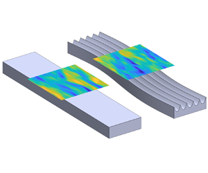
 $^{-1}$ energy, 15 Hz repetition rate) operated in dual pulse mode was used to illuminate the tracing particles. The laser beam was shaped into a thin sheet of less than 1 mm thickness using a combination of spherical and cylindrical lenses. The final thickness was refined further using a mask connected to the wind tunnel wall. The illuminated region was centred with respect to the removable plate, as indicated schematically in figure 1.

Figure 1. Schematic representation of the test section with detail of the removable plate. The track of the laser sheet, indicated in green, is not to scale. The inset reports a representative snapshot with the indication of the streamwise and spanwise extents of the measurement region.

Figure 2. Detail of the parabolic profile of the grooves: (a) isometric view, and (b) top view. One wavelength  $\lambda$ is represented in the figure for the sake of clarity.
One Andor Zyla 5.5 Mpixel sCMOS camera (sensor size  $2560 \times 2160$ pixel, pixel size
  $6.5 \mathrm {\mu }$m) was used to capture the images of the tracing particles. The camera was equipped with a Nikkor 200 mm Micro lens, operated at a value of the aperture
  $f_\#=11$. The acquisition frequency was set to 15 Hz. The imaged area extended for 21 mm in the streamwise direction (
 $x$) and 23 mm in the cross-stream direction (
 $z$). The corresponding value of the digital resolution was approximately 93 pixel mm
 $^{-1}$.
The flow was seeded upstream of the stagnation chamber using HAZEBASE Base M Fog Fluid. The small droplets of diameter  $1 \ \mathrm {\mu }$m were generated using a SAFEX Fog generator. For each Reynolds number and each plate, 2000 pairs of images were acquired. The raw images were pre-processed using a proper orthogonal decomposition approach to reduce to a minimum the spurious reflection within the illuminated region (Mendez et al. Reference Mendez, Raiola, Masullo, Discetti, Ianiro, Theunissen and Buchlin2017).
The vector fields were obtained by processing the collected images using a correlation-based algorithm. A spline interpolation of the image and of the velocity field was performed, as recommended by Astarita (Reference Astarita2006, Reference Astarita2008). A Blackman weighting window was used to tune the spatial resolution (Astarita Reference Astarita2007). The algorithm is based on a multi-pass approach, and the final interrogation window size was  $48 \times 48$ pixel, with 75 % overlap. The resulting vector spacing is approximately
  ${3.03} l_\tau$ at
  $Re_\theta =2200$ and
  ${4.54} l_\tau$ at
  $Re_\theta =2900$.
3. Results
3.1. Manipulation of the LSS
The wall-parallel PIV data allowed the investigation of how the surface roughness manipulates the turbulent structures that are typical of the boundary layer. In particular, the focus of this investigation was the analysis of the LSS.
The first step of the investigation was concerned with the detection of the LSS. It is worth mentioning that for the high-speed streaks, a similar procedure can be applied.
The detection of the LSS was based on the definition of a threshold on the local value of the streamwise velocity, as suggested by Iuso et al. (Reference Iuso, Di Cicca, Onorato, Spazzini and Malvano2003) and Schoppa & Hussain (Reference Schoppa and Hussain2002). Regions of streamwise fluctuating velocity  $u(x_i,z_i) < -u_{thr}$ are first identified in the image. For the present investigation,
  $u_{thr} = 0.5 u_\tau$. Within each identified region, the (
 $x_c, z_c$) locations of local minima of
  $u$ in
  $z$ are identified as streak centres. The
  $z$ positions where
  $u$ exhibits a zero-crossing are recognized as the streak borders. Furthermore, the spanwise distance between the centroids of the two closest LSS detected within a snapshot is defined as the streaks’ spacing
  $\lambda _z$. The procedure is then repeated for all the streaks educed from each snapshot.
Different approaches were also tested, such as the one described by Lin et al. (Reference Lin, Laval, Foucaut and Stanislas2008) based on the ratio between the mean and the standard deviation of the streamwise velocity, which led to similar results.
As evidenced in previous investigations (Choi Reference Choi2002; Iuso et al. Reference Iuso, Di Cicca, Onorato, Spazzini and Malvano2003; Quadrio & Ricco Reference Quadrio and Ricco2004; Ricco Reference Ricco2004; Yao, Chen & Hussain Reference Yao, Chen and Hussain2019), active flow control techniques such as the spanwise oscillation of the wall can lead to significant variations in the statistical distribution of the near wall streaks. Variations are also expected in the present investigations, although more limited due to the fact that the control technique is passive, and as such, it yields much lower values of drag reduction.
Following the eduction approach described above, the streaks’ spacing  $\lambda _z$ and their width
  $w_S$ are analysed initially. A statistical description of the two parameters, streaks’ spacing (
 $\lambda _z^+$) and width (
 $w_S^+$), is instrumental to determine the effect of the wall manipulation on the structure of the boundary layer. It is worth mentioning explicitly that the quantities are normalized in inner units using the values of the friction velocity calculated for each case from a Clauser fit applied to the logarithmic region of the mean velocity profile measured by Cafiero & Iuso (Reference Cafiero and Iuso2022). In figure 3, the probability density functions (p.d.f.s) of
  $\lambda _z^+$ and
  $w_S^+$ obtained from the Smooth, RLong, RS1 and RS2 cases at the two investigated values of
  $Re_\theta$ are reported. At the lowest value of
  $Re_\theta$, corresponding to
  $s^+\approx 7$, the effect of the manipulation is only weakly evidenced on the distributions of the LSS spacing (
 $\lambda _z^+$), as reported in figure 3(a). In particular, the effect of the ribbed geometry, regardless of the specific manipulation, is such that larger values of the streaks’ spacing are less probable. The peak of the p.d.f., which is found at
  $\lambda _z^+\approx 130$ for the Smooth case, shifts towards smaller values at
  $\lambda _z^+\approx 110$. The limited variations of the p.d.f. are in good agreement with the direct measurements of the friction drag reported in table 3. Indeed, the RS cases yielded small values of the drag reduction, with similar values attained also with the RLong case.

Figure 3. Probability density function of the streaks’ (a,c) spacing and (b,d) width. Data are collected at (a,b)  $Re_\theta =2200$ and
  $y^+=35$, (c,d)
  $Re_\theta =2900$ and
  $y^+=50$.
Similar considerations can also be drawn for the streaks’ width (figure 3b), at  $Re_\theta =2200$. The main difference in the p.d.f.s can be found in the fact that ribbed geometries yield greater probabilities of streaks width in the range of values between 25 and 45. The p.d.f.s of both spacing and width show a similar behaviour, with a horizontal shift of the curves for all the manipulated cases towards lower values of both
  $\lambda _z^+$ and
  $w_S^+$.
At  $Re_\theta =2900$, corresponding to
  $s^+\approx 11$, the sinusoidal riblets were found to be more effective in terms of drag reduction than the longitudinal ones, as documented in table 3. The effectiveness in terms of drag reduction is also reflected in a more prominent manipulation of the LSS.
The p.d.f.s of the streaks’ spacing are reported in figure 3(c). Both the Smooth and RLong cases show a peak at  $\lambda _z^+\approx 110$, which is in good agreement with the literature on the topic. The sinusoidal cases, instead, show a rather different behaviour. The p.d.f. is skewed towards smaller values of
  $\lambda _z^+$, peaking at
  $\lambda _z^+\approx 110$. Small differences are instead evidenced between RS1 and RS2 cases. Moreover, the streaks’ spacing values greater than
  $\lambda _z^+\approx 150$ are less probable in the sinusoidal cases.
The p.d.f.s of the streaks’ width obtained at  $Re_\theta =2900$, corresponding to
  $s^+\approx 11$, are reported in figure 3(d). While the Smooth and RLong cases feature distributions of the width that are not significantly different from those reported in figure 3(b), this is not so for the sinusoidal cases. In particular, the p.d.f. exhibits a plateau in the range of
  $w_S^+$ between 25 and 45, with a corresponding lower probability of finding streaks with values of
  $w_S^+$ greater than 50.
On the basis of the results presented above, a first summary of the effect of the manipulation can be drawn. In the sinusoidal cases, the LSS are closer together and thinner. This effect increases at values of  $s^+$ where the RS cases are more effective in reducing drag. This effect will be linked to the drag reduction mechanism later in the paper.
The conditional averages of the mean streamwise velocity and wall-normal vorticity profiles, calculated across the streaks, can provide further evidence of the topology of the streaky structures.
Figure 4 shows the conditionally averaged streamwise velocity fluctuations ( $\hat {u}^+$) and wall-normal vorticity (
 $\hat {\omega }_y^+$) profiles. Starting from the streak's centre (
 $z_c$) at all the streamwise locations corresponding to a streak, the streamwise velocity and wall-normal vorticity values in the range
  $-70< z-z_c<70$ are stored and then averaged over all the educed streaks.

Figure 4. Conditionally averaged (a,c) streamwise velocity fluctuations and (b,d) wall-normal vorticity profiles, calculated across the LSS. Data are collected at (a,b)  $Re_\theta =2200$ and
  $y^+=35$, (c,d)
  $Re_\theta =2900$ and
  $y^+=50$.
The profiles are plotted in a reference frame that is centred on the streak,  $(z-z_c)^+$. Here and in the following, the hat symbol will be used to indicate that the average is performed on points belonging to the identified LSS.
At  $Re_\theta =2200$, both the streamwise velocity and the wall-normal vorticity profiles do not show significant differences between the investigated cases. Figure 4(a) shows that all cases exhibit a velocity deficit associated with the presence of the LSS, at least concerning RS2. The RS cases are characterized by a narrower profile, attaining a plateau at smaller values of
  $|(z-z_c)^+|$. The wall-normal vorticity profiles reported in figure 4(b) highlight these differences further. The sinusoidal cases are characterized by a steeper slope of the
  $\hat {\omega }_y^+$ profile at
  $(z-z_c)^+=0$. Furthermore, even though only limited differences are detectable, the spanwise distance between the peaks is reduced in the RS cases, consistently with results reported in figure 3(b). Indeed, this distance can be associated with the typical streaks’ width.
At  $Re_\theta =2900$, which corresponds to
  $s^+\approx 11$, much clearer differences can be detected between the investigated cases. The sinusoidal cases evidence a stronger velocity deficit in the centre of the streak (figure 4c). Correspondingly, the above-mentioned narrower profile of the streak is further evidenced at values of
  $s^+$ yielding higher values of drag reduction (see table 3).
The conditional averaged wall-normal vorticity profiles (figure 4d) show these differences further. In particular, the sinusoidal cases exhibit a much steeper gradient at the centre of the streak, associated with a narrower velocity profile. Differently from the case at a lower Reynolds number, the sinusoidal case also evidences larger values of the peak with respect to the Smooth and RLong cases. Even though the differences between the RS1 and RS2 cases are small, the results seem to suggest an effect of the amplitude of the sinusoidal pattern; nevertheless, a broader parametric space, with more investigated amplitudes  $a$, is needed to support this observation. The results of figures 4(b) and 4(d) show that the sinusoidal riblets enhance the wall-normal vorticity at the streaks’ edges, with corresponding large values of in-plane shear.
Further insights into the effect of the riblet geometry can be evidenced by analysing the p.d.f. of the modulus of the in-plane projection of the velocity gradient,  $|\boldsymbol {\nabla } \hat {u}|_{x,z}$, calculated in correspondence of the LSS edges. Figures 5(a) and 5(b) further support the conclusions that have been drawn when discussing the conditional velocity and vorticity profiles.

Figure 5. Probability density functions of the modulus of the velocity gradient ( $|\boldsymbol {\nabla } \hat {u}|_{x,z}$) projected on the
  $x$–
$x$– $z$ plane calculated at the streaks’ edges, for (a)
  $Re_\theta =2200$ and
  $y^+=35$, (b)
  $Re_\theta =2900$ and
  $y^+=50$.
The riblet cases at  $Re_\theta =2200$ (figure 5a) show a shift towards greater values of the peak of the modulus of the velocity gradient. In particular, the RLong, RS1 and RS2 cases feature an increased probability of
  $|\boldsymbol {\nabla } \hat {u}|_{x,z}>0.12$. This suggests that the riblet cases are generally characterized by more intense shear regions; furthermore, the amplitude of the sinusoidal geometry seems to introduce even stronger values of the velocity gradients.
At larger values of the Reynolds number,  $Re_\theta =2900$, the RLong case features a behaviour that closely resembles the Smooth case. Conversely, the p.d.f.s of
  $|\boldsymbol {\nabla } \hat {u}|_{x,z}$ in the sinusoidal cases are characterized by a shift of the peak towards greater values of
  $|\boldsymbol {\nabla } \hat {u}|_{x,z}$, in agreement with the larger values of wall-normal vorticity evidenced in figure 4.
The p.d.f. of the conditional wall-normal vorticity calculated at the edges of the LSS is reported figure 6. At  $Re_\theta =2200$, the effect of the riblet geometry is such that smaller values of vorticity become less probable, with a corresponding increment of the probability associated with the tails of the p.d.f., namely for
  $|\hat {\omega }_y^+|>0.15$. Correspondingly, the peak of the p.d.f. shows a progressive shift towards larger values of
  $|\hat {\omega }_y^+|$ when the manipulated cases are considered.

Figure 6. Probability density functions of the wall-normal vorticity  $\hat {\omega }_y$ calculated at the streaks’ edges. Data are collected at (a)
  $Re_\theta =2200$ and
  $y^+=35$, (b)
  $Re_\theta =2900$ and
  $y^+=50$.
At  $Re_\theta =2900$, the RS cases show a much clearer distinction with respect to both the Smooth and RLong cases. In particular, the RS cases lead to a shift in the maxima of the p.d.f. towards greater values of
  $|\hat {\omega }_y^+|$. In addition to this, a higher probability of occurrence of values
  $|\hat {\omega }_y^+|>0.08$ is detected, with a trend that seems to suggest the effect of the amplitude of the sinusoidal riblet. On the other hand, the RLong case features a p.d.f. of the wall-normal vorticity that closely resembles that of the Smooth case.
Schoppa & Hussain (Reference Schoppa and Hussain2002), using transient growth analysis of the streaks, have shown that large values of  $\omega _y$ are generally associated with streaks that are more prone to instability, and as such give rise to streamwise vortices. In the present case, the greater values of wall-normal vorticity can be responsible not only for the streaks’ instability but also for their fragmentation and/or weakening.
Table 4 summarizes the number of educed streaks for each of the investigated cases. In particular, the results are presented in the form of percentage variation with respect to the Smooth case ( $\Delta N_{S} = 100\times (N_{S} - N_{S}^{S})/N_{S}^{S}$), where
  $N_{S}$ indicates the number of streaks in the ribbed cases, and
  $N_{S}^{S}$ the number of educed streaks in the Smooth case. The results seem to suggest that there is a fundamentally different behaviour when comparing the RLong with the RS cases. The latter indeed show a consistent increase in the number of the streaks with respect to the Smooth case. At larger values of the Reynolds number, which correspond to higher effectiveness of the riblets in terms of drag reduction, the number of educed streaks increases.
Table 4. Percentage variation of the number of educed LSS. The smooth case is taken as a reference.

The results presented in figures 3 and 4, and table 4, allow us to further elaborate on the mechanism by which sinusoidal riblets manipulate the near-wall turbulence. The sinuous geometry leads to streaks that are characterized by larger values of the wall-normal vorticity. This makes the LSS more prone to instability, thus causing their fragmentation. The fragmentation is reflected in two different aspects: (i) more streaks are educed in the RS cases; (ii) the mean spacing between streaks, as well as their width, is reduced in the RS cases.
Cafiero & Iuso (Reference Cafiero and Iuso2022) suggested a possible mechanism leading to the drag reduction evidenced by the sinusoidal riblets, which was associated with the imprint of the geometry manipulation onto the flow field. The spatial periodic inversion triggered by the sinusoidal geometry yields secondary flows and a cross-stream velocity component with an inverted direction at each bend. This mechanism leads to enhanced wall-normal vorticity, along with possible effects on the streamwise and spanwise vorticity that need further analysis in future investigations. The results presented in this paper support the previous hypothesis, linking the fragmentation of the LSS to the spatial variation of vorticity.
A statistical analysis based on two-point correlations of the velocity fluctuations in the wall-parallel ( $x$–
$x$– $z$) plane will serve the purpose of elucidating the effects of the wall manipulations on the structure of the LSS.
The two-point correlation between any two quantities  $A$ and
  $B$ is defined as
 \begin{equation} R_{AB}(\Delta x, \Delta z)= \frac{\overline{A(x,z)\,B(x+\Delta x,z+\Delta z)}}{\sigma_A \sigma_B}, \end{equation}
where  $\sigma _A$ and
  $\sigma _B$ are the standard deviations of
  $A$ and
  $B$, respectively, and
  $\Delta x$ and
  $\Delta z$ are the in-plane separations between the two components. The overbar notation indicates the ensemble average operation over the acquired snapshots. It is worth mentioning that the current analysis is carried out considering that the location at which the correlation is computed is beyond the roughness layer, and as such, homogeneity can be assumed in
  $x$ and
  $z$. Following Cheng et al. (Reference Cheng, Wong, Hussain, Schröder and Zhou2021) and Modesti et al. (Reference Modesti, Endrikat, Hutchins and Chung2021), we estimate the value of the roughness layer as
  $\delta _r^+ = 0.62 s^+$, which in the most limiting case,
  $Re_\theta =2900$, corresponds to
  $\delta _r^+=6.57$.
Figure 7(a) shows the two-point correlation  $R_{uu}$ calculated at
  $Re_\theta =2900$ and
  $y^+=50$, corresponding to the case where the sinusoidal riblets yield the largest values of drag reduction. The contour shows the representative Smooth case, whilst figure 7(b) shows the comparison between the four investigated cases for two generic values of the contour line (
 $R_{uu}=0.5$ solid line, and
  $R_{uu}=0.2$ dashed line) for the four investigated cases.

Figure 7. (a) Contour plot of the normalized two-point correlations  $R_{uu}$ calculated for the Smooth case. (b) Comparison between the four investigated cases for two generic contour lines:
  $R_{uu}=0.5$ (solid line)
  $R_{uu}=0.2$ (dashed line). Data are collected at
  $Re_\theta =2900$ and
  $y^+=50$.
The Smooth case exhibits iso-lines of the correlation that are elongated in the streamwise direction, which are characteristic of the existence of the low- and high-speed streaks. The RLong case shows a behaviour that is comparable with the Smooth case, with a more elongated correlation lobe, and same width; this result is in good agreement with the data shown in figure 3, which reported values of the streaks’ spacing and width that are similar between the Smooth and RLong cases. It is important to point out that the streamwise extent of the iso-lines of correlation is limited by the size of the illuminated region (see § 2). Therefore, it is not surprising if the extent of the correlation map in the streamwise location is sharply interrupted, at least for the Smooth case, in correspondence with  $\Delta x^+\approx 1000$.
The sinusoidal cases show an altered structure of the two-point correlation maps: both the streamwise and spanwise extents of the correlation lobe are indeed reduced. The amplitude of the riblet seems to play a role in how the correlation map is modified: larger values of the amplitude correspond to reduced extents of the correlation maps. This is confirmed quantitatively in table 5, where the values of the streamwise integral length scale ( $L_x^+$) are calculated by integrating the
  $R_{uu}$ correlation map (figure 7) at
  $\Delta z^+=0$ and reported. In this case, the RLong case yields values of
  $L_x^+$ greater than those attained by the Smooth wall (about 17.1
  $\%$). On the other hand, both sinusoidal cases feature a reduction in the streamwise extent of the correlation, of 6.9
  $\%$ and 25.4
  $\%$ for RS1 and RS2, respectively. A possible explanation for the opposite behaviour between the RLong and RS cases might be associated with a different underlying physics that leads to the drag reduction. The same trend is indeed retrieved also in the values of the spanwise correlation length
  $L_z^+$, calculated by integrating the
  $R_{uu}$ correlation map (figure 7) at
  $\Delta x^+=0$. The effect of the surface manipulation on
  $L_z^+$ is quite striking, with the sinusoidal cases featuring a significant reduction. This behaviour is consistent with the manipulation of the near-wall structures by means of the surface geometry, which in turn leads to attenuated and less energetic structures. A possible interpretation for this result can be found in the mechanism leading to the fragmentation of individual structures when manipulated. The effect of the ribbed surface is indeed such that LSS are weakened and, as already pointed out when discussing the p.d.f. of the streaks’ spacing (
 $\lambda _z^+$), brought closer together. This is associated with the reduced values of
  $L_z^+$. This mechanism is represented schematically in figure 8.

Figure 8. Schematic representation of the fragmentation occurring in the case of sinusoidal manipulation.
Table 5. Values of the longitudinal ( $L_x^+$) and lateral (
 $L_z^+$) integral length scales calculated for the four investigated cases at
  $Re_\theta =2900$ and
  $y^+=50$.

The effect of the sinusoidal geometry on the structure of the turbulent boundary layer is further confirmed by the analysis of the  $R_{uw}$ correlation maps (figure 9). The contour plot shows two lobes of correlation of opposite sign, located on either side of
  $\Delta z^+=0$. The positive (negative) correlation lobe is located at
  $\Delta z^+>0$ (
 $<0$). For the representative condition of LSS (
 $u<0$), the positive lobe of correlation corresponds to a negative spanwise velocity (
 $w<0$), i.e. an entrainment towards the centre of the streak. An opposite behaviour can be envisaged instead for the negative correlation lobe. The distance between the two peaks indicates a measure of the streaks’ width. The results are indeed consistent with the description: the spanwise extent of the correlation lobe reduces for the manipulated cases, with RS2 attaining the smallest size.

Figure 9. (a) Contour plot of the normalized two-point correlations  $R_{uw}$ calculated for the Smooth case. (b) Comparison between the four investigated cases for one generic contour line,
  $R_{uw}=\pm 0.04$ (solid/dashed line, respectively). Data are collected at
  $Re_\theta =2900$ and
  $y^+=50$.
3.2. The VISA conditional averages
The confirmation of the fragmentation mechanism can be sought in the conditional averages calculated across the edges of the low- and high-speed streaks. The edges of the streaks are characterized by strong velocity gradients in the streamwise and spanwise directions, and they are generally associated with values of the local variance of the velocity that are greater than the variance calculated over the entire dataset. When the latter condition is verified, an event is identified.
The approach that has been followed is based on VISA (Johansson, Alfredsson & Kim Reference Johansson, Alfredsson and Kim1991), which represents the spatial counterpart of the variable interval temporal average (VITA) (Blackwelder & Kaplan Reference Blackwelder and Kaplan1976). Each instantaneous image is divided into a structured grid. The size of each cell of the grid is then defined, and for the present investigation, a streamwise extent  $\Delta \tilde {x}^+=200$ and spanwise extent
  $\Delta \tilde {z}^+=100$ have been considered, corresponding to numbers of grid points
  $n_x$ and
  $n_z$ in the streamwise and spanwise directions, respectively. At each index
  $(i,j)$ of the grid, the value of the local variance of the streamwise velocity is computed as
 \begin{equation} \overline{{u}^2}^+_{loc} = \frac{1}{n_x n_z}\sum_{i=1}^{n_x} \sum_{j=1}^{n_z} (u^+(i,j))^2-\left(\frac{1}{n_x n_z}\sum_{i=1}^{n_x} \sum_{j=1}^{n_z} u^+(i,j)\right)^2, \end{equation}
where  $\overline {{u}^2}^+_{loc}$ indicates a local average, calculated over the cell of extent
  $\Delta \tilde {x}^+$,
  $\Delta \tilde {z}^+$. For each instantaneous image, a corresponding map of the local variance is obtained. Locally, the points that are characterized by values of the local variance
  $\overline {{u}^2}^+_{loc}$ greater than
  $k$ times the global variance
  $\overline {u^2}^+$ (i.e. calculated over all the snapshots) are identified as VISA events:
 \begin{equation} \overline{{u}^2}^+_{loc}>k \, \overline{u^2}^+.\end{equation}
For the present investigation,  $k$ has been set to 1.
Di Cicca et al. (Reference Di Cicca, Iuso, Spazzini and Onorato2002a) argued that the VISA events that satisfy the condition of (3.3) are generally found at the edges of the streaks since those regions are characterized by large values of intermittency. Figure 10 shows a representative instantaneous realization of the flow field with overlaid locations of the VISA events. The locations of the events indeed correspond to the regions of intense shear at the edges of the streaks.

Figure 10. The VISA events detected on a representative instantaneous realization of the flow field overlaid on the colour map of the streamwise velocity fluctuation.
Among all the identified events, further conditioning is then applied. In particular, the VISA events that are characterized by  $\partial u/\partial x<0$ and
  $\partial u/ \partial z>0$ are selected. The selection of these events is purely arbitrary; indeed, by combining the streamwise and cross-stream derivatives of the streamwise velocity component, it is possible to reconstruct all the flanks of a sinuous streak.
Each of the identified events is then averaged considering a window centred on the event location, of extent  $\Delta \tilde {x}^+$ in the streamwise direction and
  $\Delta \tilde {z}^+$ in the cross-stream direction. Figure 11 shows the averaged VISA event of the cross-stream velocity component obtained for the Smooth, RLong, RS1 and RS2 cases with overlaid streamlines. The source of the streamlines is the same for all cases.

Figure 11. VISA conditionally averaged spanwise velocity ( $\tilde {w}^+$) for events characterized by
  $\partial u/\partial x<0$ and
  $\partial u/\partial z>0$, with overlaid streamlines, for cases (a) Smooth, (b) RLong, (c) RS1, and (d) RS2. Data are collected at
  $Re_\theta =2900$ and
  $y^+=50$.
Here and in the following, a tilde will be used to indicate VISA quantities. In all cases, the contour shows a region of intense shear, with values of  $\tilde {w}^+$ that change in sign when passing from
  $\tilde {x}^+<0$ to
  $\tilde {x}^+>0$, or similarly from
  $\tilde {z}^+<0$ to
  $\tilde {z}^+>0$. This leads to the consideration that the centre of the event is a region of the flow where the streamlines roll up, hence leading to large values of the wall-normal vorticity. Further to this, it can be argued that the manipulated cases show streamlines that are denser than the Smooth case, which can be addressed directly to the larger values of the wall-normal vorticity.
The VISA conditioned profiles of the streamwise ( $\tilde {u}^+$) and cross-stream (
 $\tilde {w}^+$) velocity components extracted at
  $\tilde {z}^+=0$ are reported in figures 12(a,b). As could also be inferred from the contour plots in figure 4, the effect of the manipulation is such that the ribbed geometry leads to a less intense gradient of the streamwise velocity component compared with the Smooth case. On the other hand, there is no significant difference among the manipulated cases. The cross-stream VISA profiles measured in the streamwise direction show instead an opposite trend with respect to those of figure 12(a). All the ribbed cases display an enhancement of the peak-to-peak value of
  $\tilde {w}^+$, with the longitudinal case featuring the largest values. This result seems to be at odds with results reported in § 3.1, when describing the effect of the sinusoidal riblets on the wall-normal vorticity. However, the leading term associated with the wall-normal vorticity is
  $(\partial \tilde {u}/\partial z)^+$, with
  $(\partial \tilde {w}/\partial x)^+$ being instead significantly smaller.

Figure 12. The VISA conditionally averaged streamwise ( $\tilde {u}^+$) and spanwise (
 $\tilde {w}^+$) velocity profiles extracted at (a,b)
  $z^+=0$ and (c,d)
  $x^+=0$ for VISA events characterized by
  $\partial u/ \partial x<0$ and
  $\partial u/\partial z>0$, with overlaid streamlines. Data are collected at
  $Re_\theta =2900$ and
  $y^+=50$.
To confirm that the results are indeed consistent, we show the joint p.d.f. of the velocity gradients  $(\partial \tilde {u}/\partial z)^+$,
  $(\partial \tilde {u}/\partial x)^+$ calculated for the identified events in figure 13(a). In particular, the spanwise gradient is linked to the wall-normal vorticity, while the streamwise one relates to the most energetic VISA events. The manipulated cases are characterized by greater velocity gradients
  $(\partial \tilde {u}/\partial z)^+$ in the spanwise direction, with a corresponding attenuation of the streamwise velocity gradient
  $(\partial \tilde {u}/\partial x)^+$. This is identified more clearly in figure 13(b). Indeed, consistently with the larger values of wall-normal vorticity evidenced at the streak edges by the RS cases, the p.d.f. shows that despite the similarity between the manipulated and Smooth cases, the RS ones yield a higher probability of large values of
  $(\partial \tilde {u}/\partial z)^+$.

Figure 13. (a) Joint p.d.f. of the gradient of the VISA conditioned streamwise velocity calculated along the streamwise ( $(\partial \tilde {u}/\partial x)^+$) and cross-stream (
 $(\partial \tilde {u}/\partial z)^+$) directions at the centre of each VISA event for the (i) Smooth, (ii) RLong, (iii) RS1 and (iv) RS2 cases. (b) Marginal p.d.f. of
  $(\partial \tilde {u}/\partial z)^+$. Data are collected at
  $Re_\theta =2900$ and
  $y^+=50$.
3.3. The VISA conditioned turbulent kinetic energy budget
The identification of the VISA events is further exploited to elucidate the contribution of the LSS to the production term of the turbulent kinetic energy equation. The planar PIV available for the current experiments provides us access to only some of the terms involved in the turbulent kinetic energy budget, which can be formulated as follows:
 \begin{equation} \underbrace{\frac{\bar{U}_k}{2}\,\frac{\partial \overline{q^2}}{\partial x_k}}_{\mathcal{A}} = \underbrace{-\overline{u_i^{\prime} u_j^{\prime}}\,\frac{\partial \bar{U}_i}{\partial x_j}}_{\mathcal{P}}- \underbrace{\frac{\partial}{\partial x_k} \left( \frac{\overline{u^{\prime}_k q^2}}{2}+\frac{\overline{u^{\prime}_k p}}{\rho} \right)}_{\mathcal{T}} + \underbrace{\frac{\nu}{2}\,\frac{\partial^2 \overline{q^2}}{\partial x_m^2}}_{\mathcal{D}_v}-{\varepsilon},\end{equation}
with  $q^2={u^{\prime }_i}^2$. Here,
  $\mathcal {A}$,
  $\mathcal {P}$ and
  $\mathcal {T}$ indicate the advection, production and transport of turbulent kinetic energy, while
  $\mathcal {D}_v$ and
  $\varepsilon$ indicate the viscous diffusion and dissipation due to the fluctuating rate of strain. For the present case, given the value of the Reynolds number,
  $\mathcal {D}_v$ is deemed to be negligible with respect to
  $\varepsilon$. The turbulent transport
  $\mathcal {T}$ is constituted of the triple velocity correlation
  $\overline {u^{\prime }_k q^2}$ and the pressure velocity correlation
  $\overline {u^{\prime }_k p}$.
The purpose of this subsection is to highlight the effect of the surface manipulation on the production term of the turbulent kinetic energy equation. The analysis is carried out on the detected VISA events, in order to focus on how the production and transport are affected by the surface manipulation, limited to the streaks’ edges. Given the limited spatial resolution, along with the absence of some of the terms measured with the current PIV set-up, it was not possible to provide information about the dissipation term ( $\varepsilon =2 \nu (\overline {s_{ij}s_{ij}})$). On the other hand, considering the wall-normal distance at which the measurements are taken, namely
  $y^+=50$, the transport term attains values that are close to zero (Pope Reference Pope2000) and as such can be not focal for the present investigation.
Figure 14 shows the production term ( $\tilde {\mathcal {P}}$) calculated for the Smooth, RLong, RS1 and RS2 cases from the VISA conditioned flow field, overlaid with the iso-lines of
  $\tilde {u}^+=\pm 0.5$. The effect of the surface manipulation is immediately visible in the distribution of the production term. In particular, the introduction of the ribbed surface leads to the attenuation of the production term, regarding both positive and negative terms. All the cases are characterized by two intense lobes, mostly contained within the streak. The identified iso-lines are indeed representative of the shear region between a low-speed streak and a high-speed streak: given the specific conditioning that is considered for the VISA events, which takes into account those events that are characterized by
  $\partial u/\partial z>0$ and
  $\partial u/\partial x<0$, values
  $\tilde {z}^+>0$ correspond to locations that are outside the LSS. Values
  $\tilde {z}^+=0$, i.e. the centre of the VISA events, are indeed associated with the streaks’ edge.

Figure 14. Colour map of the VISA conditionally averaged production ( $\tilde {\mathcal {P}}$), overlaid with the isolines
  $\tilde {u}^+=\pm 0.5$, for the (a) Smooth, (b) RLong, (c) RS1 and (d) RS2 cases. Data are collected at
  $Re_\theta =2900$ and
  $y^+=50$.
The analysis of the individual terms contributing to the turbulence production, reported here only for the Smooth case for the sake of brevity, shows that the leading term in the turbulence production is  $\tilde {\mathcal {P}}\approx \tilde {\mathcal {P}}_{xx}=- \overline {uu}\,\partial \bar {u}/\partial x$, while the remaining three terms (considering the available PIV measurements) are at least one order of magnitude smaller. It must be noted explicitly that the investigated plane neglects the production term that is associated with the strongest component of shear (
 $\partial \bar {u}/\partial y$) and shear stress (
 $\overline {uv}$).
The attenuation of the turbulence production in the wall-parallel plane can be ascribed to the already highlighted fragmentation of the near-wall LSS, in the cases of the sinusoidal riblets. In particular, as evidenced in figure 14(a), the Smooth case yields intense regions of positive/negative production at the streak boundaries, associated with the more intense streamwise and cross-stream shear rates in the conditional VISA events of figure 12.
All the riblet cases (figures 14b–d) are characterized by an attenuation of the turbulence production (both positive and negative). It is interesting to notice how despite there being only small differences between the longitudinal and sinusoidal cases, RLong (figure 14b) features a more intense protrusion of the turbulence production within the core of the LSS, i.e. towards  $z^+<0$ with respect to RS1 (figure 14c) and RS2 (figure 14d). Indeed, the latter cases are characterized by values of the turbulence production mostly confined at the edges of the streaks (i.e. the centre of the VISA event). This is also in line with the general observation of narrower streaks as highlighted in all the sinusoidal cases.

Figure 15. Colour maps of the components of the turbulence production (a)  $\tilde {\mathcal {P}}_{xx}$ and (b)
  $\tilde {\mathcal {P}}_{xz}$, and corresponding components of the velocity gradient (c)
  $\partial \bar {\tilde {u}}/\partial x$ and (d)
  $\partial \bar {\tilde {u}}/\partial z$ calculated over the VISA events, overlaid with the isolines
  $\tilde {u}^+=\pm 0.5$.
For one representative condition only, namely the Smooth case, figure 15 shows the comparison between the production terms associated with the normal  $\overline {\tilde {u}\tilde {u}}$ and shear
  $\overline {\tilde {u}\tilde {w}}$ stresses. In particular, figures 15(a,b) are representative of the
  ${\tilde {\mathcal {P}}}_{xx}$ and
  $\tilde {{\mathcal {P}}}_{xz}$ terms, respectively, and figures 15(c,d) give the associated values of the mean velocity gradients
  $\partial \bar {\tilde {u}}/\partial x$ and
  $\partial \bar {\tilde {u}}/\partial z$, respectively. The first immediate conclusion is that the term
  ${\tilde {\mathcal {P}}}_{xx}$ is at least one order of magnitude greater than
  ${\tilde {\mathcal {P}}}_{xz}$. This is due to the fact that despite the term
  $\partial \bar {\tilde {u}}/\partial z$ being greater than
  $\partial \bar {\tilde {u}}/\partial x$, the stress term
  $\overline {\tilde {u}\tilde {w}}$ attains values close to zero, for all the investigated cases. Conversely, the normal stress term
  $\overline {\tilde {u}\tilde {u}}$ counterbalances the smaller values of the velocity gradient
  $\partial \bar {\tilde {u}}/\partial x$, thus yielding greater production values. The comparison of the total production reported in figures 14 and 15 also shows that the regions of negative/positive production are determined mostly by the sign of
  $\partial \bar {\tilde {u}}/\partial x$. Considering the specific case of VISA events, the regions of negative production are ascribed, for example, to regions of the flow located at the boundaries between LSS and the surrounding flow. Indeed, when a fluid particle moves from the inner to the outer part of LSS, we have the local value
  $\partial \bar {\tilde {u}}/\partial x>0$, with corresponding stretching and negative production (Onorato & Iuso Reference Onorato and Iuso2001). An opposite consideration can be made for the regions of the flow characterized by
  $\partial \bar {\tilde {u}}/\partial x<0$, which yield
  $\tilde {\mathcal {P}}>0$. This mechanism is also represented schematically in figure 16. It is noteworthy that
  $\mathcal {P}_{xx}$ is the leading term within the data accessible to the current PIV set-up. Figure 17 reports the turbulence production measured in the wall-normal (
 $x$–
$x$– $y$) plane from previous experimental campaigns, at the same value of the Reynolds number,
  $Re_\theta =2900$. In this case, no conditional averages are applied to the data, thus being indicative of the full components of the Reynolds stresses and shear rates. The leading term is the one related to the wall-normal shear rate,
  $P_{xy}=-\overline {uv}\,\partial {\bar {u}}/ \partial y$.

Figure 16. Schematic representation of the relation between the velocity gradient and the values of the turbulence production.

Figure 17. Turbulence production normalized in inner units calculated in the wall-normal plane at  $Re_\theta =2900$. The data are extracted from the dataset of Cafiero & Iuso (Reference Cafiero and Iuso2022).
The data show that all the surface manipulations lead to an attenuation of the turbulence production, which is particularly significant for values  $12< y^+<70$. On the other hand, the differences evidenced between the ribbed surfaces are quite limited, with the RS1 case showing slightly smaller values than RLong and RS2, which could be considered to be within the uncertainty of the measurements.
4. Conclusion
In this paper, we analyse the effect of wall manipulation using sinusoidal riblets on the near-wall structures in a turbulent boundary layer. Wall-parallel particle image velocimetry experiments at two different values of the Reynolds number ( $Re_\theta =2200$ and
  $2900$) allow us to carry out conditional averages to characterize the effect of different wall manipulations on low-speed streaks (LSS) and on the VISA events. The analysis reveals that when the sinusoidal riblets cases have efficiency similar to the RLong case in reducing drag (
 $s^+=7.06$), all the investigated cases feature a similar trend of the conditional streamwise velocity and wall-normal vorticity. Conversely, at
  $Re_\theta =2900$, corresponding to the value of
  $s^+$ yielding the largest drag reduction values (
 $s^+= 10.6$), the conditionally averaged velocity profiles of the educed LSS depart significantly from the Smooth case when the sinusoidal manipulation is considered. Namely, the streaks profile becomes narrower, with corresponding larger values of the wall-normal vorticity. This behaviour is not evidenced in the RLong case, which follows a trend similar to the Smooth case, thus suggesting that the drag reduction mechanism of the RS cases is inherently different with respect to the RLong case.
The statistical description of the LSS also shows that the RS cases lead to their fragmentation at  $Re_\theta =2900$, with a corresponding substantial increment of their number (about 24 % in RS1 and 31.5 % in RS2, respectively) compared to the Smooth case, which agrees with the reduced spacing
  $\lambda _z^+$ between LSS. This is further confirmed by the two-point correlation analysis, which highlights how in the case
  $Re_\theta =2900$, the RS cases lead to a substantial effect on the streamwise correlation and, even more significantly, the cross-stream correlation.
The fragmentation of the LSS occurring under the sinusoidal manipulation can be attributed to the periodic transversal flow generated by the sinuous grooves. In fact, the periodic spanwise flow inversion not only modifies the wall-normal vorticity, as shown extensively in this paper, but is also expected to tamper with the streamwise and spanwise vorticity components. The manipulation mechanism of the near-wall flow associated with the sinusoidal riblets seems to add further complexity to the widely accepted wall-normal displacement of the near-wall structures that characterizes the longitudinal grooves. Further investigations are ongoing to confirm these points, but there seems to be enough evidence in support of the effect of the amplitude on how the ribbed geometry manipulates the turbulent structures: the structures appear to be weakened, yet retaining an ordered structure.
Therefore, it could be argued that the effects introduced by the sinusoidal riblets resemble those of the spanwise wall oscillation, although in a much less significant fashion, the latter being an active flow manipulation.
The VISA conditional averages allowed us to describe the behaviour at the streak boundaries. We performed conditional averages to identify those events that correspond to  $\partial u/ \partial x<0$ and
  $\partial u / \partial z >0$, which is one representative flank of a streak. In the streamwise direction, VISA events are less intense, with a corresponding enhancement of the intensity in the cross-stream direction, which can be associated with the induced spanwise oscillation induced by the riblet geometry. This is particularly visible from the p.d.f. of
  $\partial u/\partial z$, which shows that a higher probability of larger spanwise gradients is associated with the sinusoidal manipulation.
The analysis of the turbulence production term applied to the VISA events reveals an attenuation for all the manipulated cases with respect to the Smooth case. In the RS cases, the turbulence production is mostly limited to the streaks’ edges, where the shear rates are significantly greater. Conversely, the Smooth and RLong cases show a more intense contribution to the turbulence production from the core of the streaks.
Acknowledgements
The authors wish to thank Professor T. Astarita for providing the software used to acquire and process the PIV images, and acknowledge F. Casagrande, S. Saggiomo and G. Virgillito for their help during the experiments.
Funding
The project has received funding from the Clean Sky 2 Joint Undertaking under the European Union's Horizon 2020 research and innovation program under grant agreement no. 945548 - GAM-2020-REG, and it was carried out within the GREENER project – funded by the European Union – Next Generation EU within the PRIN 2022 program (D.D. 104 - 02/02/2022 Ministero dell'Universit‘a e della Ricerca). This paper reflects only the authors’ views and opinions, and the Ministry cannot be considered responsible for them.
Declaration of interests
The authors report no conflict of interest.


 Open access