Ultra-short-term multi-energy load forecasting for integrated energy systems based on multi-dimensional coupling characteristic mining and multi-task learning

1 Introduction

The Integrated Energy System (IES) is a multi-energy supply system that connects multiple independent energy systems through a variety of energy coupling devices to achieve tight coupling, coordination, and complementarity between different energy forms (Alabi et al., 2022). IES can improve the flexibility of various energy systems and achieve full consumption of renewable energy and a reliable supply of multiple energy sources (Zhu et al., 2022). Therefore, the development and construction of IES is an inevitable choice to solve the energy crisis, improve environmental pollution, improve energy utilization efficiency, and promote the large-scale utilization of renewable energy (Liu et al., 2023). With the development of IES, the potential factors affecting the energy demand of IES users have gradually become more complicated, which brings huge challenges to the ultra-short-term accurate prediction of multi-load, thus affecting the optimal dispatch and demand response strategy formulation of IES (Yan et al., 2024). Therefore, it is necessary to research a more accurate ultra-short-term forecasting method for IES multi-energy loads.

In the construction phase of the input feature set for multi-energy load forecasting in IES, existing research has considered various potential factors that influence IES users’ energy consumption habits, and uses correlation analysis methods to screen the strongly correlated features for multi-energy load forecasting. Literature (Wang et al., 2022) considers the impact of meteorological information, holiday information, and temporal features on the multi-energy load when constructing the input feature set. It employs Pearson correlation analysis and Grey Relational Analysis (GRA) to select strongly correlated meteorological features for multi-energy load forecasting, thereby enhancing the forecasting model’s accuracy. Similarly, Literature (Zhuang et al., 2023) considers factors such as meteorological information and holiday information in relation to the potential association with the multi-energy load when constructing the input feature set. It utilizes Pearson correlation analysis and correlation analysis methods based on Copula theory to select strongly correlated meteorological features from both linear and nonlinear perspectives for multi-energy load forecasting. In addition, some researchers have constructed strongly correlated features that reflect the latent characteristics of multi-energy loads, achieving high prediction accuracy. For instance, Literature (Tan et al., 2023) introduces a feature selection method based on Synthesis Correlation Analysis (SCA), and constructs a Load Participation Factor (LPF) as an input feature for the prediction model, illustrating the degree of participation of each load in the total load. However, existing multi-energy load forecasting methods for IES have not fully explored the potential complex coupling characteristics between multi-energy loads of the integrated energy system in different dimensions during the input feature set construction phase, thereby leaving room for improvement in the model’s prediction accuracy.

In the construction phase of forecasting models for multi-energy loads in IES, some existing studies build separate forecasting models for different types of loads. Literature (Zheng et al., 2023) proposes a multi-energy load forecasting method based on Temporal Convolutional Networks (TCN) and global attention mechanism, forecasting electric, cooling, and heating loads separately. Literature (Ge et al., 2021) introduces a Wavelet Neural Networks (WNN) multi-energy load forecasting model based on Improved Particle Swarm Optimization (IPSO) and Chaos Optimization Algorithm (COA), which forecasts electric, cooling, and heating loads individually. Literature (Liu et al., 2022) presents a multi-energy load forecasting method combining Multivariate Phase Space Reconstruction (MPSR) with Support Vector Regression (SVR), achieving good forecasting results by separately constructing forecasting models for each load. However, there is a complex coupling relationship among the multi-energy loads in IES. The mentioned research method uses historical data of various types of loads, which are strongly correlated with the load to be predicted, as input features for the forecasting model during the construction of the input feature set. This approach only considers the coupling relationship among the multi-energy loads at the construction phase of input feature set construction and fails to fully explore the potential coupling characteristics among the multi-energy loads during the construction phase of the forecasting model. As a result, this leads to the need for improvement in the accuracy of multi-energy load forecasting.

To address this issue, some studies have employed multi-energy load forecasting models based on Multi-Task Learning (MTL), achieving high prediction accuracy. For instance, Literature (Guo et al., 2022) developed a multi-energy load forecasting model based on MTL and Bi-directional Long Short-Term Memory Networks (BiLSTM), effectively extracting potential coupling information between loads. Literature (Wang et al., 2021) used a forecasting model combining MTL with Long Short-Term Memory Networks (LSTM) to forecast the trend curves of decomposed and reconstructed multi-energy loads. Additionally, it employed the Least Squares Support Vector Regression (LSSVR) method to forecast fluctuation curves. The final multi-energy load forecast results were obtained by superimposing the predictions of the two models. However, existing studies on multi-energy load forecasting based on MTL often employ LSTM and their variants to construct the sharing layers in MTL. Although these structures contain temporal memory units, they still face issues with forgetting historical information. Furthermore, their capability to mine potential temporal associations and long-term dependencies within data is relatively weak, limiting the improvement in the accuracy of multi-energy load forecasting.

Selecting appropriate weights for the loss functions of each sub-task in the construction and training process of MTL models is a crucial means of enhancing the overall performance of the model. Current research methods on multi-energy load forecasting in IES using MTL models typically set the weights of each forecasting task’s loss function manually without adjustment. For example, Literature (Zhang et al., 2023) manually set the loss function weights for the model when utilizing MTL to construct an electric load forecasting model. Literature (Wu et al., 2022) developed a multi-energy load forecasting model for IES based on MTL and LSTM, where the loss function weights for the MTL model were manually set based on the peak ratio of different types of loads within the IES. However, manually setting the weights of the MTL loss functions during the training process will consume a considerable amount of time for parameter tuning. Additionally, setting model parameters manually may lead to one or more tasks dominating the model training process. This method of parameter configuration fails to balance the losses of the sub-tasks reasonably, lacks scientific rigor, and limits further enhancements in the prediction performance of MTL models.

To address the aforementioned issues, this paper proposes an ultra-short-term multi-energy load forecasting method based on multi-dimensional coupling characteristic mining and multi-task learning. The specific contributions of this paper are as follows:

(1) A multi-dimensional coupling characteristic mining method for multi-energy loads is employed, integrating multiple correlation analysis methods. By utilizing Pearson correlation coefficients, Spearman rank correlation coefficients, and the Maximum Information Coefficient (MIC), load features that describe the coupling relationships between multi-energy loads are constructed. This effectively quantifies the complex coupling relationships among the historical sequences of IES multi-energy loads, thoroughly mining the potential coupling characteristics from different dimensions in the construction of the input feature set.

(2) An ultra-short-term multi-energy load forecasting model based on MTL and TCN is constructed. During the model construction phase, the sharing layer of MTL is used to fully exploit the potential complex coupling characteristics among multi-energy loads. The use of dilated causal convolutions and residual connections in TCN extracts the latent temporal information of input features, capturing the long-term dependencies of the input time series.

(3) An optimization method for the forecasting model based on homoscedastic uncertainty (HU) for MTL loss function weight optimization is employed. By learning the homoscedastic uncertainty of multiple forecasting tasks, the method automatically tunes the weight parameters of the loss function, saving time on parameter tuning while further enhancing the model’s prediction performance.

(4) An experimental analysis is conducted using the IES of Arizona State University as a case study. The results demonstrate that the proposed forecasting method achieves higher prediction accuracy compared to other methods.

2 Multi-energy load characteristic analysis

The various energy subsystems in IES coordinate and complement each other through energy conversion devices, leading to complex coupling relationships among different forms of energy within IES. Simultaneously, changes in external factors such as meteorological conditions can influence the energy consumption habits of IES users, implying that the variation trends of IES multi-energy loads follow certain latent patterns. To fully explore the latent characteristics of IES multi-energy loads, this study analyzes the multi-energy load characteristics using historical data of loads from March 2018 to February 2019 from the IES of the Tempe campus of Arizona State University.

2.1 Analysis of the annual variation trends of multi-energy loads

Figure 1 displays the annual data curves of electric, cooling, and heating loads in IES from March 2018 to February 2019. To facilitate the analysis of the variation trends of multi-energy load sequences in different seasons, the load data from March to May are categorized as Spring data, June to August as Summer data, September to November as Autumn data, and December to the following February as Winter data. As indicated in Figure 1, both electric and cooling loads gradually increase to higher levels in Spring and Summer, with significant fluctuations in these two seasons. The electric load exhibits stronger fluctuations in autumn, while the fluctuations are more subdued in winter. The cooling load remains relatively stable in both autumn and winter. Conversely, the heating load shows an opposite annual trend, gradually decreasing in Spring and Summer with less variability. In Autumn and Winter, the heating load increases to higher levels with more pronounced fluctuations. This demonstrates that for the same load, the variation trends in different seasons are significantly influenced by varying meteorological and other external factors. The differences in load variation trends across different seasons imply that IES users have varying energy consumption habits in different seasons. Ignoring these differences can lead to a failure to fully explore the potential characteristics of multi-energy loads. Therefore, in conducting ultra-short-term forecasting of multi-energy loads, it is crucial to mitigate the negative impact of the differences in load variation trends between seasons on prediction accuracy.

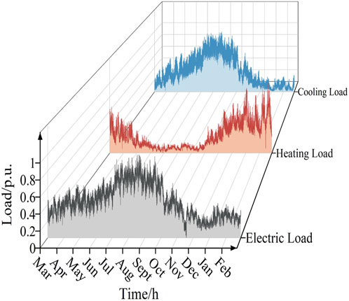
Figure 1. The annual historical data curves of multi-energy loads.

2.2 Coupling analysis between multi-energy load

Figure 1 also reveals that within the same season, the variation trends of different loads in IES are either similar or complementary, which preliminarily indicates a tight coupling relationship among IES multi-energy loads. To analyze the coupling among multi-energy loads more intuitively, Figure 2 employs the Pearson correlation analysis method to quantify the correlation of the annual variation trends among different loads. The Pearson correlation coefficient is a statistical metric that measures the degree of linear correlation between two continuous variables, and its specific expression is as follows:

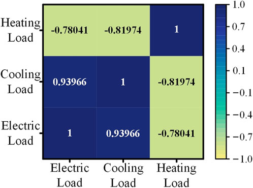
Figure 2. Pearson correlation analysis results between multi-energy loads.

In the formula, $a_i$ and $b_i$ respectively represent the i-th sample of the multi-energy load sequences A and B, while $\overline{a}$ and $\overline{b}$ represent the mean values of the multi-energy load sequences A and B, respectively. The symbol “n” denotes the total number of samples in the load sequences. The value of $\rho$ ranges from [-1, 1], and a larger value of $\left|\rho \right|$ indicates a stronger correlation.

According to Figure 2, there is a positive correlation between the IES electric load and the cooling load, while there is a negative correlation between the heating load and both the cooling and electric load. The absolute values of the Pearson correlation coefficients between the annual electric load, cooling load, and heating load in the IES are all greater than 0.7. This indicates a strong coupling relationship between the various loads in the IES. Therefore, in conducting ultra-short-term forecasts of multiple loads, it is crucial to thoroughly explore the complex coupling characteristics between these loads, as this can significantly enhance the accuracy of the forecasts.

2.3 Multi-energy loads temporal correlation analysis

The Autocorrelation Coefficients Function (ACF) is used to analyze the temporal correlation of multi-energy loads, with the results presented in Figure 3. The calculation formula for ACF is as follows:

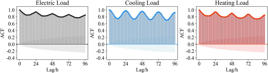
Figure 3. Annual multi-energy load autocorrelation coefficient.

In the formula, k represents the time lag, where $X_t$ denotes the load value at time t; $\mathit{\mu }$ represents the mean of the historical load sequence, and ${\mathit{\sigma }}^{\mathbf{2}}$ represents the variance of the historical load sequence. The autocorrelation coefficient takes values within the range [-1, 1], where a higher autocorrelation coefficient indicates a stronger correlation.

Figure 3 shows the autocorrelation coefficients of IES multi-energy loads with a 96-h lag, where the shaded area represents the 95% confidence interval. The figure reveals that within each 24-h lag period, the autocorrelation coefficients of the various loads first decrease and then increase, exhibiting a strong daily periodicity. Additionally, the peak values of the autocorrelation coefficients within each 24-h lag period gradually decrease. This indicates that the load values of the IES at a given moment are not only strongly correlated with the load values of adjacent times but also with the load values at the same time on adjacent days. Therefore, when conducting ultra-short-term forecasts of multi-energy loads, it is essential to fully consider the temporal correlation of the loads to achieve accurate ultra-short-term predictions.

3 Multi-dimensional multi-energy load coupling characteristics mining and input feature set construction

Section 2.2 quantifies the coupling relationships between multi-energy loads in the IES using the Pearson correlation analysis method, indicating a strong coupling among the IES multi-energy loads. However, the Pearson correlation analysis method can only describe the linear relationships between two types of load sequences and fails to capture the nonlinear relationships between loads. Therefore, this chapter employs Pearson, Spearman, and MIC correlation analysis methods to construct multi-energy load coupling features. By utilizing multiple correlation analysis methods to quantify various types of linear and nonlinear relationships between multi-energy loads, it is possible to fully explore the complex coupling characteristics among multi-energy loads from multiple dimensions. Based on this, considering various potential characteristics of multi-energy loads, an input feature set for the ultra-short-term forecasting model is constructed.

3.1 Multi-dimensional multi-energy load coupling characteristics mining based on the integration of multiple correlation analysis methods

The Spearman’s rank correlation coefficient is a non-parametric rank statistic used to measure the strength of the monotonic relationship between two continuous variables. For the multi-energy load sequences A and B, its specific expression is as follows:

In the formula, $d_i$ represents the difference in ranks between the i-th sample $a_i$ and $b_i$ in the multi-energy load sequences A and B. The value of r ranges from [-1,1], and a larger value of $\left|r\right|$ indicates a stronger correlation.

MIC measures the linear and nonlinear relationships between two continuous variables by calculating the maximum normalized mutual information under different grid divisions. MIC exhibits robustness to samples containing noise. The mutual information calculation formula between multi-energy load sequences A and B is as follows:

In the formula, $P\left(a,b\right)$ represents the joint probability density of multi-energy load sequences A and B, while $P\left(a\right)$ and $P\left(b\right)$ respectively denote the marginal probability densities of multi-energy load sequences A and B.

A grid is partitioned on the two-dimensional variable (A, B) formed by the multi-energy load sequences A and B, and the mutual information size between each grid is calculated. MIC is the maximum value of the normalized mutual information under different grid partitioning methods. Its calculation formula is as follows:

In the formula, m and n respectively represent the number of intervals partitioned in the direction of multi-energy load sequences A and B, D is the total number of grids, typically taken as D = n^0.6. The value of $\delta$ ranges from [0, 1], and a larger value of $\delta$ indicates a stronger correlation.

For a multi-energy load sequence of length n, the Pearson correlation coefficient quantifies the linear relationship between multi-energy loads by calculating covariance and standard deviation. The Spearman rank correlation coefficient quantifies simple monotonic nonlinear relationships between multi-energy loads by calculating the correlation coefficients between the ranks of variables. Meanwhile, MIC effectively measures the strength of both linear and nonlinear relationships between multi-energy loads by calculating the maximum normalized mutual information under different grid partitioning methods. Pearson, Spearman, and MIC correlation analysis methods can quantify different types of linear and nonlinear relationships between multi-energy loads. Therefore, combining these three correlation analysis methods to construct multi-energy load coupling features can measure the potential coupling relationships between loads from different dimensions, thereby fully exploring the multi-dimensional coupling characteristics between multi-energy loads.

Therefore, for the forecast moment t, the historical multi-energy load sequences from t-1 to t-s are analyzed using Pearson, Spearman, and MIC correlation methods. The obtained correlation coefficients are then averaged in a weighted manner according to formula (6), thus obtaining the IES multi-energy load coupling features at time t. These features reflect the coupling characteristics of the historical multi-energy load sequences from t-1 to t-s across different dimensions, effectively quantifying the potential complex coupling relationships between historical IES multi-energy load sequences.

To analyze the feasibility of the proposed method for mining multi-dimensional multi-energy load coupling characteristics based on the integration of multiple correlation analysis methods, let’s consider constructing multi-energy load coupling features using historical multi-energy load data from the month preceding the forecast moment as an example. The constructed multi-energy load coupling features and the load sequences are then analyzed using Pearson, Spearman, and MIC correlation methods, with the results shown in Figure 4. In the figure, S_EC, S_EH, and S_CH represent the coupling features of the electric load with the cooling load, the electric load with the heating load, and the cooling load with the heating load, respectively.

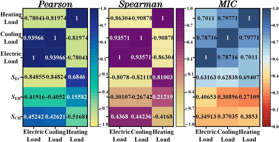
Figure 4. Correlation analysis results between coupling features and multi-energy loads.

To avoid the one-sidedness of strong correlation features obtained by using a single correlation analysis method, when the constructed coupling feature and a certain type of load in the multi-energy loads simultaneously satisfy formula (7) (Guo et al., 2022; Li et al., 2022; Chen et al., 2023), then that coupling feature is considered a strong correlation feature for the multi-energy loads.

As can be seen from Figure 4, when constructing multi-energy load coupling features using the historical load data from the month preceding the forecast moment, S_EC, S_EH, and S_CH can all be considered strong correlation features for multi-energy load prediction. This fully demonstrates the effectiveness of the proposed method for constructing multi-energy load coupling features. Furthermore, analyzing the correlation between multi-energy loads using different correlation analysis methods further indicates the strong coupling relationships within IES multi-energy loads. Using the constructed coupling features as input features for the multi-energy load forecasting model can achieve multi-dimensional mining of potential complex coupling characteristics in the construction phase of input feature set, improving the prediction accuracy of ultra-short-term multi-energy load forecasting.

3.2 Construction of multi-energy load input feature set

To avoid the negative impact of seasonal differences in load variation trends on the accuracy of multi-energy load forecasting,the historical data of loads for the entire year are divided according to different seasons. This seasonal historical data, along with other features, are collectively used as inputs for the model to build ultra-short-term forecasting models for multi-energy loads in different seasons. To fully explore the potential complex coupling relationships between multi-energy loads from multiple dimensions, the constructed coupling features S_EC, S_EH, and S_CH are subjected to correlation analysis with the multi-energy loads. If the correlation analysis results with a certain type of load satisfy Eq. 7, they are considered as input features for the multi-energy load forecasting model. Simultaneously, as meteorological factors can influence users’ energy consumption habits, meteorological features whose correlation analysis results with a certain type of load in the multi-energy loads satisfy Eq. 7 are selected as strongly correlated meteorological features for the multi-energy load. The correlation analysis results between atmospheric pressure, temperature, relative humidity, wind direction, precipitable water, dew point, and multi-energy loads are presented in Figure 5.

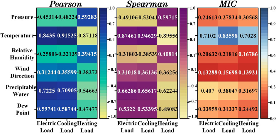
Figure 5. Correlation analysis results between meteorological features and multi-energy loads.

From Figure 5, it is evident that atmospheric pressure, temperature, precipitable water, and dew point can be considered as strongly correlated meteorological features for multi-energy load forecasting. Additionally holidays information reflecting users’ energy usage behaviors, along with time features, are also included as input features for the forecasting model. Since this study uses the IES of Arizona State University in the United States for forecasting research, it adopts the U.S. federal holidays (including New Year’s Day, Christmas, Thanksgiving, etc.) as the selection rule for holidays in the dataset. To fully consider the temporal correlation of multi-energy loads, historical load data from moments t-1 to t-3, as well as t-24, t-48, and t-72, are used as historical load features in the forecasting model, thus ensuring thorough mining of the temporal correlations of multi-energy loads.

In summary, for the multi-energy loads at the predicted time t, the input feature set for the ultra-short-term forecasting model of multi-energy loads, considering the potential characteristics of multi-energy loads, is presented as shown in Table 1.

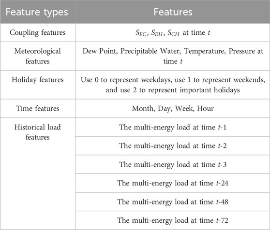
Table 1. Input feature set for each seasonal forecasting model.

4 Construction of multi-energy load forecasting

This paper develops an ultra-short-term multi-energy load forecasting model based on MTL-TCN-HU. Firstly, an MTL model based on a hard parameter sharing mechanism is employed in the model construction phase to fully mine the coupling characteristics of multi-energy loads. Secondly, the sharing layer based on TCN effectively extracts potential temporal association information from the input features and captures long-term dependencies in the input sequence. Lastly, the use of a homoscedastic uncertainty-based MTL loss function weight optimization method enables the automatic tuning of loss function weight parameters. This approach not only reduces the time cost of model parameter tuning but also further enhances the prediction accuracy of the MTL forecasting model.

4.1 MTL forecasting model based on hard parameter sharing mechanism

For the prediction of IES multi-energy loads, the approach of constructing separate load forecasting models for different types of loads does not deeply explore the potential complex coupling characteristics among various energy loads in the model construction phase. MTL enhances the predictive performance of the model by extracting coupling information from different forecasting tasks. This approach not only facilitates parallel learning of multiple forecasting tasks but also aims to improve the accuracy of the forecasting model and enhance its generalization ability (Zhang and Yang, 2022).

MTL is primarily divided into hard parameter sharing and soft parameter sharing mechanisms based on the type of sharing mechanism. Figure 6 presents the structural diagrams for both soft and hard parameter sharing mechanisms. In the soft parameter sharing mechanism, the models and parameters for each forecasting task are distinct and regularization is required before sharing potential coupling information for each sub-task. The hard parameter sharing mechanism involves different forecasting tasks learning the potential coupling information between sub-tasks directly through the same sharing layer, thereby facilitating joint training of multiple tasks. Given that the soft parameter sharing mechanism has more relaxed constraints compared to the hard parameter sharing mechanism, it is more suitable for multi-energy load forecasting tasks where the sub-tasks have weaker interrelations. In contrast, the hard parameter sharing mechanism, with its common sharing layer for each sub-task, is apt for multi-energy load forecasting tasks where sub-tasks are closely related. Since the IES multi-energy loads under study exhibit strong coupling, this paper opts for a hard parameter sharing mechanism-based MTL method to construct an ultra-short-term multi-energy load forecasting model.

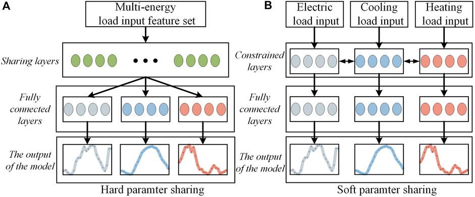
Figure 6. The structure of (A) hard parameter sharing mechanism and (B) soft parameter sharing mechanism.

4.2 Construction of MTL sharing layer based on TCN

TCN is a convolutional neural network that integrates Dilated Causal Convolution (DCC) and Residual Connection (RC). DCC includes dilated convolution and causal convolution. In TCN, causal convolution ensures that the forecasting results at earlier time steps do not involve future data information, preventing future information leakage, and making the convolutional network suitable for multi-energy load forecasting models. The dilated convolution in TCN addresses the issue of the limited receptive field in traditional convolution. Introducing a dilation coefficient d, increases the model’s receptive field while reducing the computational load, thus enabling the learning of global information. Assuming the model’s input sequence is $X=\left\{x_1,x_2,\cdots ,x_n\right\}$ and the filter is $F=\left\{f_1,f_2,\cdots ,f_{k-1}\right\}$, the calculation formula for the dilated convolution is as follows:

In the formula, k represents the filter size, d is the dilation factor, and $F\left(t\right)$ is the result of the dilated convolution for the t-th element in the input sequence.

The residual block of TCN consists of a DCC layer, WeightNorm layer, ReLu activation function, and Dropout layer. The residual block effectively addresses the issue of gradient vanishing in deep network structures and enhances the model’s generalization ability. Its core idea is to form an RC by combining the direct mapping of the input with the output of the last layer of the residual module, thereby improving the model’s stability and facilitating the construction of deep networks. An example of a DCC structure with d = 1, 2, 4, and k = 3 is shown in Figure 7. In the figure, $\widehat{Y}=\left\{{\widehat{y}}_1,{\widehat{y}}_2,\cdots ,{\widehat{y}}_n\right\}$ represents the output of the DCC.

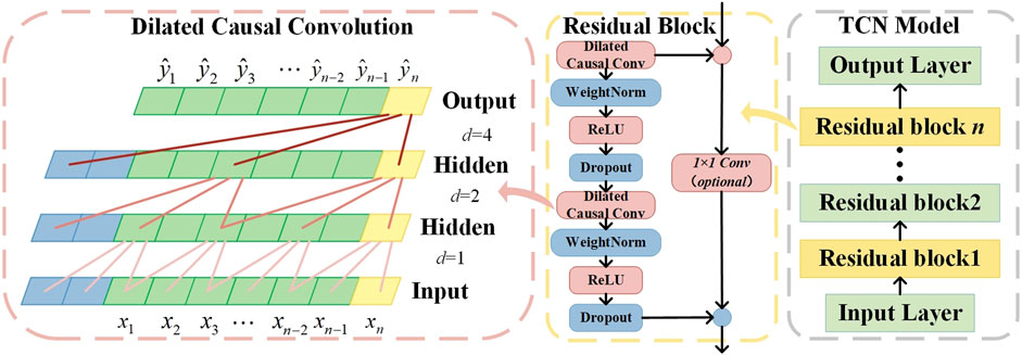
Figure 7. The structure of TCN model.

From Figure 7, it is evident that TCN can capture long-term dependencies in the input time series while avoiding the problem of gradient vanishing. It possesses a strong capability to mine the potential temporal association information in the input data. Therefore, this paper opts to use TCN to construct the sharing layer of the MTL model.

4.3 Method for optimizing the weight of MTL loss functions based on homoscedastic uncertainty

MTL models achieve parallel learning of multiple sub-tasks through the sharing mechanisms of the model. The loss function of MTL is as shown in Eq. 9:

In the formula, L represents the loss function of MTL, r is the number of sub-tasks in MTL, $\left\{L_1,L_2,\cdots ,L_r\right\}$ denotes the loss functions of each sub-task in the MTL model and $\left\{{\lambda }_1,{\lambda }_2,\cdots ,{\lambda }_r\right\}$ represents the weights of the loss functions for each sub-task.

According to formula (9), the weights of the loss functions for sub-tasks can affect the training effectiveness of the MTL model. Scientific and rational allocation of weights to the sub-task loss functions can further enhance the performance of the multi-task learning model. Therefore, this paper adopts a homoscedastic uncertainty-based optimization method for the multi-task learning loss function.

Homoscedastic uncertainty refers to the type of uncertainty that is independent of input data. This uncertainty remains constant across all inputs and varies between different tasks, reflecting the inherent learning difficulties of each sub-task in MTL. The optimization method for MTL loss functions based on homoscedastic uncertainty is achieved by learning the homoscedastic uncertainty among different sub-tasks, thereby enabling the automatic tuning of loss function weights. Assuming an MTL model with three sub-tasks has parameters W, and the noise parameters for different tasks are ${\sigma }_1$, ${\sigma }_2$, and ${\sigma }_3$, the total loss function $L\left(W,{\sigma }_1,{\sigma }_2,{\sigma }_3\right)$ of MTL can be represented as follows:

In the formula, ${\sigma }_i^2\left(i=1\cdots 3\right)$ represents the observation noise, which is used to measure the homoscedastic uncertainty of each forecasting task, and $\ln \left({\sigma }_1{\sigma }_2{\sigma }_3\right)$ is the regularization term that restricts the model from learning in the direction of unbounded increase of ${\sigma }_i^2$.

4.4 The overall framework of the forecasting model

The framework of the ultra-short-term multi-energy load forecasting model is shown in Figure 8. It mainly comprises the following three parts:

(1) Multi-dimensional multi-energy load coupling characteristics mining: Selecting the length s of the historical load sequence for correlation analysis, calculating the Pearson correlation coefficient, Spearman correlation coefficient, and MIC between the multi-energy load historical sequences from t-1 to t-s, and using formula (6) to integrate various correlation analysis methods to construct the multi-energy load coupling features at time t. This approach quantifies the complex coupling relationships between multi-energy loads and enables in-depth multi-dimensional mining of potential couplings in the construction phase of the multi-energy load input feature set.

(2) Construction of multi-energy load input feature set: Dividing the annual historical data of multi-energy loads by different seasons, to construct ultra-short-term forecasting models for multi-energy loads in various seasons. Various correlation analysis methods are used to select strongly correlated features from coupling and meteorological features, which are then combined with holiday features, time features, and historical load features to form the multi-energy load input feature set. This method comprehensively considers various factors affecting the energy usage habits of IES users and deeply mines the potential characteristics of multi-energy loads.

(3) Construction of multi-energy load forecasting model: An ultra-short-term multi-energy load forecasting model based on MTL-TCN-HU for IES is constructed. The MTL model based on a hard parameter sharing mechanism extracts coupling information between sub-tasks through the sharing layer, enabling in-depth mining of potential complex coupling characteristics among multi-energy loads during the model construction phase. TCN, using DCC and RC, extracts potential temporal association information from input features and captures long-term dependencies in the input time series. The HU multi-task learning loss function weight optimization method, by learning the homoscedastic uncertainty of different tasks, achieves automatic tuning of loss function weight parameters, thereby saving time in model tuning and further enhancing the accuracy of multi-energy load forecasting.

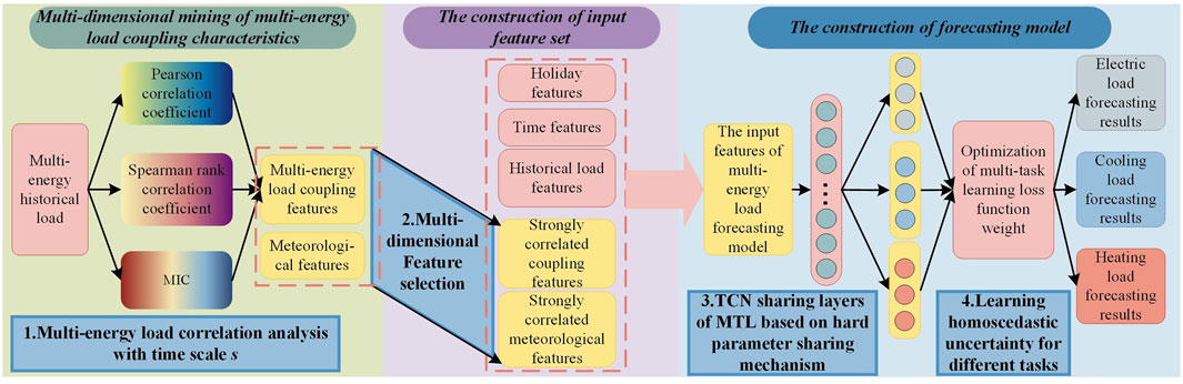
Figure 8. The structure of ultra-short-term multi-energy load forecasting model.

5 Case study

5.1 Data source and evaluation index

This paper selects historical data on electric, cooling, and heating loads from the comprehensive energy system of Arizona State University’s Tempe campus, spanning from 1 March 2018, to 28 February 2019, for training the ultra-short-term forecasting model. The multi-energy load data are divided according to different seasons, and then each season’s load data are split into training, validation, and test sets in the ratio of 8:1:1. The meteorological data are sourced from the National Solar Radiation Database of the United States.

This paper selects Mean Absolute Error (MAE), Mean Absolute Percentage Error (MAPE), Root Mean Square Error (RMSE), and Weighted Mean Absolute Percentage Error (WMAPE) as the forecasting error evaluation metrics, and their calculation formulas are as follows:

In the formula, $y_i$ represents the actual load value, $\widehat{y_i}$ denotes the forecasting load value, and n indicates the number of samples. ${\theta }_E$, ${\theta }_C$, and ${\theta }_H$ represent the prediction error weights for electric, cooling, and heating loads, respectively. They are set to 0.4, 0.4, and 0.2 (Wu et al., 2022), respectively. $MAP{E}_E$, $MAP{E}_C$, and $MAP{E}_H$ represent the MAPE for electric, cooling, and heating loads. Lower values of MAE, MAPE, and RMSE imply higher accuracy of the model’s predictions.

5.2 Experimental platform and data preprocessing

The construction and training of the forecasting model are based on the Pytorch deep learning framework. The hardware configuration of the experimental platform includes an Intel(R) Core (TM) i7-12700H CPU, with acceleration provided by an NVIDIA GeForce RTX3060 Laptop GPU.

The 3 $\sigma$ rule is used to filter out anomalies in the historical multi-energy load data, treating these anomalies as missing data, which are then filled using cubic spline interpolation. To eliminate the impact of input feature dimensions on the forecasting model, max-min normalization is applied to ensure that the input data range is between [0,1].

5.3 Comparative analysis of forecasting methods

5.3.1 Selection of load sequence length for constructing coupling features

The method of mining multi-dimensional multi-energy load coupling characteristics based on the integration of multiple correlation analysis methods involves analyzing the correlation of the historical multi-energy load sequences from t-1 to t-s to construct the coupling features of multi-energy loads at time t. Therefore, it is crucial to appropriately select the length of the multi-energy load historical sequence used for constructing coupling features. If a shorter load sequence is chosen to construct coupling features, the randomness and volatility of the multi-energy loads may result in significant changes in coupling features between adjacent time steps. The strong fluctuations in the sequence prevent the coupling feature sequence from fully reflecting the potential coupling relationships among multi-energy loads. On the other hand, if a longer load sequence is chosen to construct coupling features, the changes in coupling features between adjacent time steps are relatively small. Consequently, the sequence of coupling features for multi-energy loads exhibits a more gradual change trend, also failing to capture the potential coupling relationships. To select an appropriate length for the multi-energy load sequence to construct coupling features, experiments are conducted using historical load data from 29 November 2017, to 28 February 2019.

Different lengths of multi-energy load sequences, specifically 1 week, 2 weeks, 3 weeks, 1 month (31 days), 2 months (61 days), and 3 months (92 days), are selected to construct coupling features as input features for the forecasting model. The ultra-short-term prediction accuracy of multi-energy loads is compared and analyzed using the MAPE. To facilitate the construction of multi-energy load coupling features and to ensure that the selected sequence lengths effectively reflect the potential coupling relationships of multi-energy loads 1 month, 2 months, and 3 months prior to the predicted moment, the load sequence lengths for 1 month, 2 months, and 3 months were defined as the number of days with the highest occurrence frequency for 1 month, 2 months, and 3 months, respectively, in the dataset from March 2018 to February 2019, which are 31 days, 61 days, and 92 days, respectively. The related parameters of the experiment are presented in Table 2. To comprehensively assess the prediction effects of different sequence lengths, data from 1 week in different seasonal test sets are used for ultra-short-term multi-energy load forecasting, with specific experimental results shown in Figure 9.

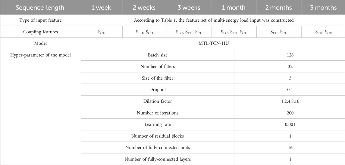
Table 2. Experimental input features and model parameters for selecting load sequence length used in constructing coupling features.

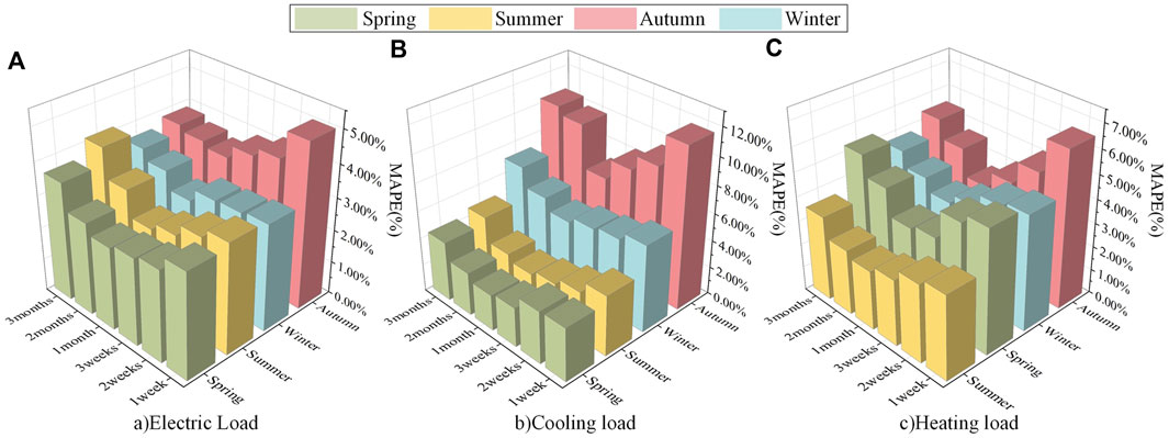
Figure 9. Comparative MAPE chart for the experiment on selecting load sequence length used in constructing coupling features.

As Figure 9 indicates, when multi-energy load coupling features are constructed using historical sequence lengths of 1 week, 2 weeks, 3 weeks, and 1 month, the prediction error of the models for each season decreases with the increase in the length of the load sequence used for constructing coupling features. However, when using 1 month, 2 months, and 3 months as the historical sequence lengths, the prediction error increases with the length of the load sequence. The MAPE, RMSE, and MAE of the forecasting models are the lowest when a 1-month multi-energy historical load sequence is used for constructing coupling features. This suggests that coupling features constructed with a 1-month load sequence effectively quantify the complex coupling relationships between multi-energy loads. Therefore, the historical multi-energy load sequence length of 1 month prior to the forecast moment is chosen for constructing the coupling features at the forecast moment, making it the input feature of the model, thereby better achieving in-depth multi-dimensional mining of the potential coupling characteristics of multi-energy loads.

5.3.2 Ablation experiment

To validate the effectiveness of each component of the proposed forecasting method, comparative experiments are designed as shown in Table 3. Models 0, 1, and 2 all use the approach of constructing separate forecasting models for different types of loads and select strongly correlated features as input features for each load forecasting model. Among these, Model 0 does not include coupling features as input for the forecasting model, and Model 1 does not use the TCN model for multi-energy load prediction. Models 3 and 4 both employ MTL models for prediction. Model 3 does not use the homoscedastic uncertainty-based MTL loss function weight optimization method, and its loss function weights are manually set (Wu et al., 2022). Model 4 represents the multi-energy load forecasting method proposed in this paper. Data from 1 week in different seasonal test sets are used for ultra-short-term multi-energy load forecasting, and the forecasting results of each model for different seasons are evaluated using MAPE, RMSE, and MAE. The forecasting results of each model are presented in Tables 4–6.

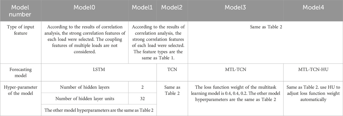
Table 3. Ablation experiment input features and model parameters.

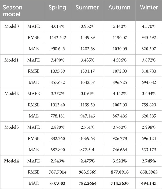
Table 4. Comparison of prediction errors in electric load forecasting results of different models.

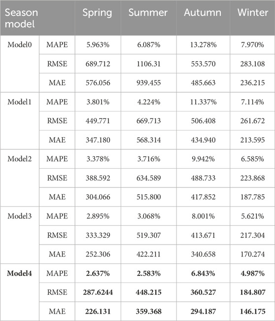
Table 5. Comparison of prediction errors in cooling load forecasting results of different models.

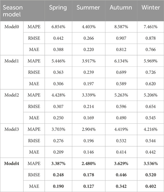
Table 6. Comparison of prediction errors in heating load forecasting results of different models.

From Tables 4–6, it is evident that Model 4 achieves the highest ultra-short-term prediction accuracy for multi-energy loads across different seasons. Additionally, there is a gradual increase in the ultra-short-term prediction accuracy of multi-energy loads from Model 0 to Model 4. Compared to Model 0, Model 1 shows a decrease in the MAPE of electric load by 12.330%–15.273%, cooling load by 10.740%–36.257%, and heating load by 11.106%–28.566% across different seasons. This demonstrates that the proposed method for mining multi-dimensional multi-energy load coupling characteristics based on the integration of multiple correlation analyses can effectively quantify the complex coupling relationships between multi-energy loads. It achieves in-depth mining of potential coupling characteristics from various dimensions in the construction phase of the input feature set, significantly enhancing the prediction accuracy of multi-energy loads. Compared to Model 1, Model 2 shows a reduction in the MAPE of electric load by 6.246%–11.313%, cooling load by 7.436%–12.305%, and heating load by 12.783%–18.693%. This indicates that the TCN model effectively extracts potential temporal association information from input features and captures long-term dependencies in the input time series, thereby improving the accuracy of multi-energy load prediction. Compared to Model 2, Model 3 shows a reduction in the MAPE of electric load by 9.44%–12.696%, cooling load by 14.298%–19.523%, and heating load by 13.028%–19.016%. This suggests that the MTL model based on a hard shared parameter mechanism can fully mine the potential complex coupling characteristics between multi-energy loads during the model construction phase, further reducing the prediction error of the model. Compared to Model 3, Model 4 shows a decrease in the MAPE of electric load by 6.356%–12.007%, cooling load by 8.912%–15.808%, and heating load by 8.533%–17.877%. This indicates that the homoscedastic uncertainty-based MTL loss function weight optimization method can automatically tune the loss function weights by learning the homoscedastic uncertainty of different tasks, further enhancing the model’s prediction performance. Overall, each component of the proposed multi-energy load forecasting method significantly improves the prediction accuracy of multi-energy loads.

5.3.3 Comparative analysis of different prediction models

To further evaluate the prediction accuracy of the proposed model, this study compares its performance with commonly used models in existing research, including Random Forest (RF), Support Vector Regression (SVR), CNN-BiGRU, and MTL-BiGRU forecasting models. The input features and related parameters for the experiment are shown in Table 7.

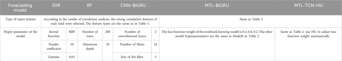
Table 7. Comparison of experimental input features and model parameters between different forecasting models.

Data from 1 week in different seasonal test sets are used for ultra-short-term multi-energy load forecasting. The MAPE prediction errors of each forecasting model in different seasons are shown in Figure 10, and the prediction result curves for each model in different seasons are presented in Figure 11. The WMAPE prediction errors of each forecasting model in different seasons are shown in Table 8. Tables 8; Figures 10, 11 reveal that in different seasons, the prediction curves of the SVR and RF models have a poor fit with the actual values. The CNN-BiGRU model can extract latent feature information and temporal associations reflecting load changes (Niu et al., 2022), but it fails to fully extract the long-term dependencies of input features and does not adequately mine the potential complex coupling characteristics between multi-energy loads, resulting in lower prediction accuracy. The MTL-BiGRU model also cannot learn long-term dependencies of input features and does not employ a scientific MTL loss function weight optimization method, leading to poor prediction performance. In contrast, the proposed forecasting model not only uses TCN to thoroughly mine potential temporal associations and long-term dependencies in the input data but also explores the potential coupling characteristics between multi-energy loads through an MTL model based on a hard parameter sharing mechanism. Additionally, it achieves scientific parameter optimization through a homoscedastic uncertainty-based MTL loss function weight optimization method. Therefore, the proposed forecasting model exhibits the highest prediction accuracy across different seasons.

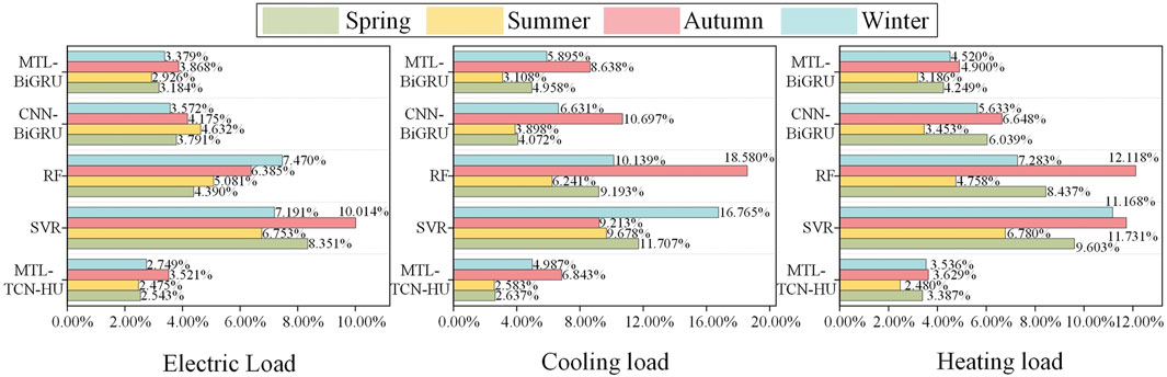
Figure 10. MAPE comparison chart of different forecasting models.

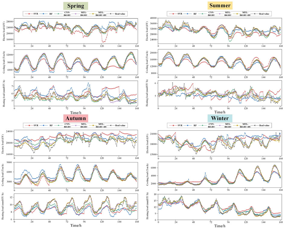
Figure 11. Forecast results of each model in different seasons.

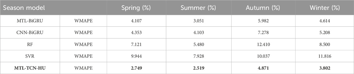
Table 8. Comparison of WMAPE for different forecasting models.

6 Conclusion

This paper proposes an ultra-short-term multi-energy load forecasting method based on multi-dimensional coupling characteristic mining and multi-task learning. Firstly, a multi-dimensional multi-energy load coupling characteristics mining method, integrating multiple correlation analysis methods, is employed to construct load coupling features. This effectively quantifies the complex coupling relationships between IES multi-energy loads and thoroughly mines potential coupling characteristics from various dimensions in the input feature set construction phase. Case studies show that using this method in different seasons results in a decrease in the MAPE of electric load by 12.330%–15.273%, cooling load by 10.740%–36.257%, and heating load by 11.106%–28.566%.

Then, an ultra-short-term multi-energy load forecasting model based on MTL and TCN is constructed, which mines the potential complex coupling characteristics between multi-energy loads during the model construction phase. The TCN is used to mine potential temporal association information from input features and capture long-term dependencies in the input time series. Case studies indicate that employing MTL reduces the MAPE of electric load by 9.44%–12.696%, cooling load by 14.298%–19.523%, and heating load by 13.028%–19.016% in different seasons. Using TCN results in a decrease in the MAPE of electric load by 6.246%–11.313%, cooling load by 7.436%–12.305%, and heating load by 12.783%–18.693%.

Moreover, a homoscedastic uncertainty-based MTL loss function weight optimization method is adopted to automatically tune the loss function weight parameters, saving time in model tuning while further enhancing the model’s prediction performance. Case studies show that employing this method results in a decrease in the MAPE of electric load by 6.356%–12.007%, cooling load by 8.912%–15.808%, and heating load by 8.533%–17.877% in different seasons.

Finally, a comparative analysis of different forecasting models is conducted using the comprehensive energy system of Arizona State University in the United States as a case study. The results indicate that the proposed forecasting method has higher prediction accuracy compared to other methods.

Data availability statement

Publicly available datasets were analyzed in this study. This data can be found here: https://nsrdb.nrel.gov/data-viewer, http://cm.asu.edu/.

Author contributions

NH: Conceptualization, Data curation, Formal Analysis, Supervision, Writing–original draft. XW: Data curation, Investigation, Methodology, Validation, Writing–original draft. HaW: Methodology, Project administration, Software, Writing–review and editing. HeW: Resources, Software, Visualization, Writing–review and editing.

Funding

The author(s) declare that financial support was received for the research, authorship, and/or publication of this article. This research was funded by China’s National Key Development Plan, grant number 2022YFB2404002.

Conflict of interest

The authors declare that the research was conducted in the absence of any commercial or financial relationships that could be construed as a potential conflict of interest.

Publisher’s note

All claims expressed in this article are solely those of the authors and do not necessarily represent those of their affiliated organizations, or those of the publisher, the editors and the reviewers. Any product that may be evaluated in this article, or claim that may be made by its manufacturer, is not guaranteed or endorsed by the publisher.

References

Alabi, T. M., Aghimien, E. I., Agbajor, F. D., Yang, Z., Lu, L., Adeoye, A. R., et al. (2022). A review on the integrated optimization techniques and machine learning approaches for modeling, prediction, and decision making on integrated energy systems. Renew. Energy 194, 822–849. doi:10.1016/j.renene.2022.05.123
Chen, H., Zhu, M., Hu, X., Wang, J., Sun, Y., and Yang, J. (2023). Research on short-term load forecasting of new-type power system based on GCN-LSTM considering multiple influencing factors. Energy Rep. 9, 1022–1031. doi:10.1016/j.egyr.2023.05.048
Ge, L., Li, Y., Yan, J., Wang, Y., and Zhang, N. (2021). Short-term load prediction of integrated energy system with wavelet neural network model based on improved Particle Swarm optimization and Chaos optimization Algorithm. J. Mod. Power Syst. Clean. Energy 9 (6), 1490–1499. doi:10.35833/mpce.2020.000647
Guo, Y., Li, Y., Qiao, X., Zhang, Z., Zhou, W., Mei, Y., et al. (2022). BiLSTM multitask learning-based combined load forecasting considering the loads coupling relationship for multienergy system. IEEE Trans. Smart Grid 13 (5), 3481–3492. doi:10.1109/tsg.2022.3173964
Li, C., Li, G., Wang, K., and Han, B. (2022). A multi-energy load forecasting method based on parallel architecture CNN-GRU and transfer learning for data deficient integrated energy systems. Energy 259, 124967. doi:10.1016/j.energy.2022.124967
Liu, H., Tang, Y., Pu, Y., Mei, F., and Sidorov, D. (2022). Short-term load forecasting of multi-energy in integrated energy system based on multivariate phase Space reconstruction and support vector regression mode. Elect. Power Syst. Res. 210, 108066. doi:10.1016/j.epsr.2022.108066
Liu, Y., Li, Y., Li, G., Lin, Y., Wang, R., and Fan, Y. (2023). Review of multiple load forecasting method for integrated energy system. Front.Energy Res. 11. doi:10.3389/fenrg.2023.1296800
Niu, D., Yu, M., Sun, L., Gao, T., and Wang, K. (2022). Short-term multi-energy load forecasting for integrated energy systems based on CNN-BiGRU optimized by attention mechanism. Appl. Energy 313, 118801. doi:10.1016/j.apenergy.2022.118801
Tan, M., Liao, C., Chen, J., Cao, Y., Wang, R., and Su, Y. (2023). A multi-task learning method for multi-energy load forecasting based on synthesis correlation analysis and load participation factor. Appl. Energy 343, 121177. doi:10.1016/j.apenergy.2023.121177
Wang, C., Wang, Y., Ding, Z., Zheng, T., Hu, J., and Zhang, K. (2022). A transformer-based method of multienergy load forecasting in integrated energy system. IEEE Trans. Smart Grid 13 (4), 2703–2714. doi:10.1109/tsg.2022.3166600
Wang, S., Wu, K., Zhao, Q., Wang, S., Feng, L., Zheng, Z., et al. (2021). Multienergy load forecasting for regional integrated energy systems considering multienergy coupling of variation characteristic curves. Front.Energy Res. 9. doi:10.3389/fenrg.2021.635234
Wu, K., Gu, J., Meng, L., Wen, H., and Ma, J. (2022). An explainable framework for load forecasting of a regional integrated energy system based on coupled features and multi-task learning. Prot. Control Mod. Power Syst. 7 (1), 24. doi:10.1186/s41601-022-00245-y
Yan, Q., Lu, Z., Liu, H., He, X., Zhang, X., and Guo, J. (2024). Short-term prediction of integrated energy load aggregation using a bi-directional simple recurrent unit network with feature-temporal attention mechanism ensemble learning model. Appl. Energy 355, 122159. doi:10.1016/j.apenergy.2023.122159
Zhang, S., Chen, R., Cao, J., and Tan, J. (2023). A CNN and LSTM-based multi-task learning architecture for short and medium-term electricity load forecasting. Elect. Power Syst. Res. 222, 109507. doi:10.1016/j.epsr.2023.109507
Zhang, Y., and Yang, Q. (2022). A survey on multi-task learning. IEEE Trans. Know. Data Eng. 34 (12), 5586–5609. doi:10.1109/tkde.2021.3070203
Zheng, Q., Zheng, J., Mei, F., Gao, A., Zhang, X., and Xie, Y. (2023). TCN-GAT multivariate load forecasting model based on SHAP value selection strategy in integrated energy system. Front. Energy Res. 11. doi:10.3389/fenrg.2023.1208502
Zhu, J., Dong, H., Zheng, W., Li, S., Huang, Y., and Xi, L. (2022). Review and prospect of data-driven techniques for load forecasting in integrated energy systems. Appl. Energy 321, 119269. doi:10.1016/j.apenergy.2022.119269
Keywords: multi-dimensional coupling characteristic mining, multi-task learning, integrated energy systems, ultra-short-term multi-energy load forecasting, homoscedastic uncertainty
Citation: Huang N, Wang X, Wang H and Wang H (2024) Ultra-short-term multi-energy load forecasting for integrated energy systems based on multi-dimensional coupling characteristic mining and multi-task learning. Front. Energy Res. 12:1373345. doi: 10.3389/fenrg.2024.1373345
Received: 19 January 2024; Accepted: 27 March 2024;
Published: 11 April 2024.
Edited by:
Michael Carbajales-Dale, Clemson University, United StatesReviewed by:
Bin Zhou, Hunan University, ChinaTao Huang, Polytechnic University of Turin, Italy
Hanbo Zheng, Guangxi University, China
Copyright © 2024 Huang, Wang, Wang and Wang. This is an open-access article distributed under the terms of the Creative Commons Attribution License (CC BY). The use, distribution or reproduction in other forums is permitted, provided the original author(s) and the copyright owner(s) are credited and that the original publication in this journal is cited, in accordance with accepted academic practice. No use, distribution or reproduction is permitted which does not comply with these terms.
*Correspondence: Nantian Huang, huangnantian@neepu.edu.cn