


1. Introduction
Drop coalescence is a central dynamical mechanism in many physical settings that involve dispersions of small drops. For example, coalescence in clouds increases the size of drops, leading to rain (Pruppacher & Klett Reference Pruppacher and Klett2010), and the coalescence of ink drops on the page limits the resolution of inkjet printers (Stringer & Derby Reference Stringer and Derby2009). Consequently, the fundamental problem of coalescence between two isolated drops has been the focus of a large body of work, with many different dynamical regimes being studied theoretically (e.g. Eggers, Lister & Stone Reference Eggers, Lister and Stone1999; Duchemin, Eggers & Josserand Reference Duchemin, Eggers and Josserand2003 – referred to henceforth as ELS and DEJ, respectively), numerically (e.g. Sprittles & Shikhmurzaev Reference Sprittles and Shikhmurzaev2012, Reference Sprittles and Shikhmurzaev2014a; Anthony, Harris & Basaran Reference Anthony, Harris and Basaran2020 – referred to as SS12, SS14 and AHB, respectively) and experimentally (e.g. Aarts et al. Reference Aarts, Lekkerkerker, Guo, Wegdam and Bonn2005; Paulsen, Burton & Nagel Reference Paulsen, Burton and Nagel2011 – referred to as PBN).
One of the core questions is how the radius  $r_b(t)$ of the ‘fluid bridge’ connecting the two drops increases as coalescence proceeds from the initial point of contact. At early times (see figure 1a), the fluid bridge is much smaller than the drops, the flow is driven by a region of very large interfacial curvature at its edge, and it is reasonable to expect the sort of asymptotic scaling behaviour that is often found near interfacial singularities associated with changes in fluid topology. While
  $r_b(t)$ is the most obvious variable of interest, a fuller description would include the interfacial shape and the structure of the flow.

Figure 1. (a) Geometrical definition sketch for early-time coalescence between two initially spherical drops of radius  $a$ showing the hierarchy of length scales. The drops are joined axisymmetrically in the plane
  $z=0$ of cylindrical polar coordinates
  $(r,\theta,z)$ by a fluid bridge of radius
  $r_b(t)\ll a$. The edge of the bridge is tightly curved on a scale
  $|r-r_b|\sim r_c\ll r_b$. Ahead of the bridge, the drops are separated by a thin gap of width
  $2h(r,t)\ll r_b$. (b) Sketch of the flow structure in the inertial regime. The net force
  $2\gamma$ (per unit length into the page) from the edge creates radial momentum, which is left in a viscous wake over the fluid bridge. Entrainment into the wake with velocity
  $W$ drives an outer irrotational flow on the fluid-bridge scale, which widens the gap width
  $2h$ ahead of the fluid bridge.
For the case of very viscous drops with negligible inertia in a negligible outer fluid, there is an exact solution for the complete coalescence of two circular drops in two dimensions (Hopper Reference Hopper1984; Richardson Reference Richardson1992). Though a complete solution is possible only in this very special case due to the availability of conformal mapping techniques, ELS argued that the early-time behaviour of  $r_b(t)$ in Hopper's solution can be extended to give the same early-time asymptotic behaviour in three dimensions. Moreover, SS12 showed numerically that Hopper's full solution for
  $r_b(t)$ gives a surprisingly good approximation for the coalescence rate of inertialess spheres over much of their evolution. For drops with both viscosity and inertia, ELS argued further that the initial dynamics of coalescence is viscously dominated on the length scale of the fluid bridge, and thus also has the same leading-order asymptotic behaviour at early times. Inertia can nevertheless play a role of the length scale of the two drops (Paulsen et al. Reference Paulsen, Burton, Nagel, Appathurai, Harris and Basaran2012). In this early-time viscous regime, both the initial drop profile (AHB; Beaty & Lister Reference Beaty and Lister2022, Reference Beaty and Lister2023) and the presence of an outer fluid (ELS; Thompson & Billingham Reference Thompson and Billingham2012; SS14) can significantly alter the dynamics, for example by allowing a bubble of external fluid to accumulate at the advancing meniscus and change its curvature.
As the bridge radius increases, inertia becomes more important relative to viscosity in the bridge-scale flow. For sufficiently low viscosity drops after the initial viscous regime, or for ideal (inviscid) drops, there is also an inertial regime of coalescence in which inertial forces balance surface tension at leading order. Both ELS and DEJ considered this regime theoretically and numerically for an ideal fluid in the early-time geometry when the fluid bridge is still small compared to the macroscopic scale of the drop, as we will outline shortly. The primary purpose of this paper is to give an analytic description of the effects of small, but non-zero, drop viscosity in this early-time inertial regime.
To establish some notation, consider, as shown in figure 1(a), two axisymmetric drops of fluid with dynamic viscosity  $\mu$, density
  $\rho$ and surface tension
  $\gamma$. We assume that any outer fluid has negligible viscosity and inertia. Initially, at
  $t=0$ the drops are spheres of radius
  $a$ touching at a point. At later times, the drops are joined by a fluid bridge of radius
  $r_b(t)\ll a$ in the plane
  $z=0$ of cylindrical polar coordinates
  $(r,\theta,z)$. Ahead of the fluid bridge, the surface of the drop is given by
  $z = \pm h(r,t)$. In the far field,
  $r\gg r_b$, the surface matches to the initial spherical drop shape: hence on scales
  $r_b\ll r\ll a$, we have
  $h = r^2/2a$ to leading order. At the edge of the fluid bridge,
  $r=r_b$, the surface is tightly curved on a length scale
  $r_c\ll r_b$ given by the local radius of curvature. Consequently, surface tension exerts a large stress on the ‘tightly curved’ region
  $|r-r_b|\sim r_c$, which drives the growth of the fluid bridge.
In the inertial regime, ELS argued that the radius of curvature scales with the width of the gap in the tightly curved region, giving  $r_c\sim r_b^2/a$. Therefore, the interfacial stress due to surface tension in this region scales as
  $\gamma / (r_b^2/a)$. By assuming that this stress balances the inertial term
  $\rho |\boldsymbol u|^2$ for a flow with velocity
  $\boldsymbol u$ that scales as
  $\dot r_b \equiv {\rm d} r_b / {\rm d} t\sim r_b/t$, where
  $t$ is the elapsed time, ELS obtained the key scaling result
 \begin{equation} r_b =D \left(\frac{\gamma a }{\rho}\right)^{1/4}t^{1/2}, \end{equation}
where  $D$ is an
  $O(1)$ dimensionless prefactor, whose value is not predicted by scaling. Given the scaling (1.1), the Reynolds number
  $Re$ for the flow in the tightly curved region is
  $Re \sim r_c \dot r_b /\nu \sim r_b/( \textit {Oh} \, a)$, where
  $\nu$ is the kinematic viscosity, and
  $\textit {Oh} \equiv \mu / (\rho a \gamma )^{1/2}$ is the Ohnesorge number. The assumed inertial stress balance for flow in the tightly curved region is self-consistent if
  $Re \gg 1$ or, equivalently,
  $r_b \gg \textit {Oh} \, a$. Since
  $r_b \ll a$ at early times,
  $\textit {Oh} \ll 1$ is required for the existence of an early-time inertial regime, and drops with
  $\textit {Oh}\gg 1$ remain in the viscous regime. (In general,
  $\textit {Oh}$ describes the relative importance of viscosity and inertia for surface-tension-driven flows.)
The existence of the inertial regime, the scaling relation (1.1) and the transition to the inertial regime at bridge radius  $r_b\sim \textit {Oh}\, a$ have all been confirmed experimentally (e.g. Menchaca-Rocha et al. Reference Menchaca-Rocha, Martínez-Dávalos, Núñez, Popinet and Zaleski2001; PBN). Using electrical techniques to measure
  $r_b$, PBN found the coefficient
  $D$ to be in the range 1–1.6 for
  $0.002<\textit {Oh}<0.2$. The inertial scaling has also been confirmed numerically by simulations of the full Navier–Stokes equations, including by SS14, who found that
  $D=1.5$ holds for their early-time results.
Other experiments (Wu, Cubaud & Ho Reference Wu, Cubaud and Ho2004; Aarts et al. Reference Aarts, Lekkerkerker, Guo, Wegdam and Bonn2005) also confirmed the scaling (1.1) for the inertial regime, but with lower values of  $D$ in the range 1–1.3. However, these results were obtained by fitting (1.1) to experimental data for
  $r_b/a$ in the range 0.05–0.5, and for the larger values of
  $r_b/a$, Sprittles & Shikhmurzaev (Reference Sprittles and Shikhmurzaev2014b) showed that the azimuthal curvature at the edge of the fluid bridge significantly resists its growth. Hence the lower values of
  $D$ may simply reflect the inclusion of larger values of
  $r_b/a$ in the fits.
In numerical calculations for an ideal fluid ( $\textit {Oh} = 0$), DEJ found that the early-time inertial dynamics is given by a self-similar sequence of reconnection events. As the fluid bridge advances, capillary waves grow on the surface until there is an intersection between waves on opposing surfaces. The edge of the fluid bridge jumps outwards to the intersection point, and a bubble is trapped in the drop. Averaging over successive reconnection events (and zeroing the flow numerically at each reconnection), DEJ found that the fluid bridge evolves as (1.1) with
  $D\approx 1.6$. This is faster than some of the above results from experiments and simulations with small, but non-zero, viscosity (
 $0 < \textit {Oh} \ll 1$).
Reconnection has also been seen during the viscous regime in simulations for  $\textit {Oh}=0.01$ (SS12), though it can be suppressed by a small external viscosity (SS14), which may explain why bubble trapping has not been observed experimentally. It is not clear to us if, or when, reconnection is possible in the inertial regime for drops with small, but non-zero, viscosity. For example, in full simulations of the Navier–Stokes equations in the case
  $\textit {Oh} = 0.001$, AHB found that the capillary waves had much smaller amplitudes than in DEJ and, in particular, there were no reconnection events in these calculations. (Similarly, SS14 did not observe reconnection during the inertial regime.) For the bulk of this paper, motivated by the results of AHB, we will analyse the early-time inertial regime assuming that we are in the case of no reconnection. In § 6, we will return briefly to discussion of reconnection-driven coalescence, and outline how the flow structure that we describe for
  $\textit {Oh}>0$ might be adapted to this case and affect the results of DEJ.
The structure of our paper follows the structure of the flow shown schematically in figure 1(b), which was initially motivated by the qualitative features that we observed in figure 8 of the AHB numerical simulation for  $\textit {Oh}=0.001$ (reproduced here in figure 5a). Here, we analyse each of these features of the inertial regime in turn, and demonstrate that small, but non-zero, viscosity has a leading-order effect on the rate of coalescence. In § 2, we show that radial momentum, created by the net surface tension force acting on the tightly curved edge of the fluid bridge, is left behind by the expanding edge in a thin viscous wake, analogous to the Oseen wake behind a translating body. There is a radial mass flux in the wake, whose divergence drives entrainment into the wake from above and below. In § 3, we show that the entrainment velocity into the wake drives an irrotational Euler flow outside the wake on the fluid-bridge scale. The streamlines of this entrainment-driven outer flow originate on the free surface ahead of the fluid bridge in
  $r>r_b$, thus the outer flow opens up the gap between the drops ahead of the bridge. In § 4, we calculate the cumulative opening of the gap as the tightly curved edge of the bridge approaches a given radius, and show that this increased gap width results in a slower rate of coalescence. In § 5, we compare our theoretical predictions with previous numerical and experimental results, and we conclude with discussion in § 6.
2. The wake
In the early-time inertial regime, coalescence is driven by surface tension acting on the tightly curved region around the circular edge of the fluid bridge. Ahead of the tightly curved region, the opposing surfaces of the drop are approximately parallel, since  $\partial h / \partial r \sim r_b/a \ll 1$ for
  $r_b \ll a$. Thus surface tension acting on the surface as it turns through nearly
  $180^{\circ }$ at the edge gives a net radial force of
  $2\gamma$ per unit azimuthal length. (This result can be thought of as coming from tension
  $\gamma$ in the radial direction on each of the top and bottom surfaces, or can be calculated from an integral of
  $\gamma \kappa \boldsymbol {n}$, where
  $\kappa$ is the curvature, and
  $\boldsymbol n$ is the surface normal.)
Though the force  $2\gamma$ is distributed over the small length scale
  $r_c$, on the much larger length scale
  $r_b$, it looks like a line (or ring) force acting around the circular bridge edge and moving radially through the fluid as
  $r_b(t)$ increases. The line force creates radial momentum, and this momentum is left behind the expanding bridge edge to form a thin radially directed wake in the plane of the bridge (see figure 1b). On the bridge scale, this mechanism of wake formation by a line force is similar to wake formation in the solution for a translating point force, or ‘Oseenlet’ (Chan & Chwang Reference Chan and Chwang2000), and depends only on creation and advection of momentum. Because
  $r_c\ll r_b$, the time scale
  $r_c/\dot r_b$ of wake formation is much smaller than the time scale
  $r_b / \dot r_b$ on which the rate of coalescence
  $\dot r_b(t)$ varies. Hence the rate of coalescence is approximately constant on the local time scale of wake formation. We define
  $U(r)$ to be the value of
  $\dot r_b$ when the edge of the fluid bridge reaches
  $r$. Near the edge of the bridge, on intermediate length scales
  $r_c\ll |r-r_b|\ll r_b$, we can consider
  $U(r)$ to be constant and the bridge edge to be straight at leading order.
Hence, for simplicity, we first consider two-dimensional wake formation in Cartesian coordinates  $(x,z)$ behind a horizontal point force of strength
  $2 \gamma \boldsymbol {e}_x$ (per unit length in the third direction
  $\boldsymbol {e}_y$) that is translating at constant velocity
  $U\boldsymbol {e}_x$. We assume that the momentum generated by the force is left behind as the force translates, and that its subsequent evolution is given by viscous diffusion. The momentum is thus confined to a thin viscous wake. At a distance
  $X$ behind the force, the wake has vertical width
  $(\nu X / U)^{1/2}$ given by the distance
  $(\nu \tau )^{1/2}$ of diffusion over the time
  $\tau =X/U$ that has elapsed since the force went past.
Following Hinch (Reference Hinch1993), who considers the Oseen wake behind a solid sphere in uniform flow, we consider the momentum flux and volume flux through the wake using conservation arguments. The momentum flux across a vertical plane that is a fixed distance behind the point force is  $\rho \boldsymbol u (\boldsymbol {u}-U \boldsymbol {e_x})$ (allowing for the translating plane). Therefore, since
  $|\boldsymbol u|\ll U$ away from the tightly curved region, the total rate at which horizontal momentum is left in the wake is
  $\int \rho U u_x \, {\rm d} z$ at leading order, where
  $u_x$ is the horizontal fluid velocity. The rate at which momentum is left in the wake must also equal the applied horizontal force
  $2 \gamma$. This implies a volume flux along the wake
 \begin{equation} Q=\int u_x \, {\rm d} z = \frac{2 \gamma}{\rho U} \end{equation}
(per unit length in the transverse direction). The same argument can be applied locally to the case of a force that translates with a slowly varying velocity  $U(x)$ to produce a local volume flux
  $Q(x)$ in its wake.
Having obtained the local volume flux (2.1), we now consider volume conservation in a three-dimensional wake for, as shown in figure 2, a vertically integrated area element between  $r$ and
  $r+\delta r$, where
  $\delta r \ll r$, with angular extent
  $\delta \theta \ll 1$. The volume flux through the wake into the element at
  $r$ is
  $Q(r)\,r\, \delta \theta$, and the corresponding flux out of the element at
  $r + \delta r$ is
  $Q(r+\delta r)\, (r+\delta r)\, \delta \theta$. The difference between these terms must be balanced by entrainment into the wake. Denote the vertical entrainment velocity by
  $W(r)$, which acts over the combined area
  $\approx 2r\,\delta \theta \, \delta r$ of the top and bottom of the wake element. Then, to leading order in
  $\delta r$ and
  $\delta \theta$, conservation of volume gives
 \begin{equation} 2W(r) \, r\,\delta \theta\, \delta r = Q(r+\delta r)\,(r+\delta r)\,\delta\theta - Q(r)\,r\, \delta \theta \implies W(r)= \frac{\gamma}{\rho }\,\frac 1 r\,\frac{{\rm d}}{{\rm d} r} \frac{r}{U(r)}. \end{equation}
Figure 2. A vertically integrated area element in the viscous wake between  $r$ and
  $r+\delta r$, where
  $\delta r \ll r$, with angular extent
  $\delta \theta \ll 1$. The radial flow through the wake gives a vertically integrated flux
  $Q(r)=2 \gamma / \rho \, U(r)$ at
  $r$, which is multiplied by the length
  $r\,\delta \theta$ in the azimuthal direction to give a volume flux. The difference between the volume fluxes at
  $r$ and
  $r+\delta r$ is balanced by entrainment into the element with vertical velocity
  $u_z=- W(r)$ from above, and
  $+W(r)$ from below, which is multiplied by the area
  $r\, \delta \theta \, \delta r$ to give the volume flux.
Equation (2.2) for the entrainment velocity  $W$ applies generally to any thin axisymmetric wake with slowly varying
  $U(r)$. In the inertial regime,
  $r_b(t)$ is given by (1.1), and we can differentiate
  $r_b^2(t)$ to obtain
 \begin{equation} U(r)= \frac{D^2}{2r}\left (\frac{\gamma a}{\rho}\right)^{1/2} . \end{equation}
Substitution into (2.2) then yields
 \begin{equation} W= \frac{4}{ D^2}\left (\frac \gamma { \rho a}\right)^{1/2} . \end{equation}
For this case,  $W$ is constant in time and uniform over the fluid bridge.
3. Outer entrainment-driven flow
The entrainment velocity (2.4) drives a flow outside the wake on the fluid-bridge scale with Reynolds number  $Re \sim r_b W/\nu \sim r_b/ (\textit {Oh}\, a ) \gg 1$, since
  $r_b \gg \textit {Oh}\, a$ in the inertial regime. Therefore, viscosity is negligible, and the outer entrainment-driven flow satisfies the Euler equations
 \begin{equation} \frac{\partial \boldsymbol{u}}{\partial t} + \boldsymbol{u} \boldsymbol{\cdot} \boldsymbol{\nabla} \boldsymbol{u} =- \frac 1 \rho\,\boldsymbol{\nabla} p \quad \text{and}\quad \boldsymbol{\nabla} \boldsymbol{\cdot} \boldsymbol{u} = 0. \end{equation}
Furthermore, comparison of the unsteady  $\partial \boldsymbol {u} / \partial t$ and nonlinear
  $\boldsymbol {u} \boldsymbol {\cdot } \boldsymbol {\nabla } \boldsymbol {u}$ terms in (3.1a) shows that
 \begin{equation} \frac{|\boldsymbol{u} \boldsymbol{\cdot} \boldsymbol{\nabla} \boldsymbol{u}|}{|\partial \boldsymbol{u} / \partial t|} \sim \frac{W^2/r_b}{W/t } \sim \frac{r_b}{a} \ll 1, \end{equation}
since  $r_b \ll a$ for early-time coalescence. Therefore, the nonlinear term in (3.1a) can be neglected. Neglecting the nonlinear term, the curl of (3.1a) and the radial component of (3.1a) yield
 \begin{equation} \frac{\partial}{\partial t}\left(\nabla^2 - \frac{1}{r^2}\right)\frac{\varPsi}{r} =0 \quad \text{and}\quad \frac{\partial p}{\partial r} =\frac{ \rho}{r}\,\frac{\partial ^2 \varPsi}{\partial z\,\partial t}, \end{equation}
where  $\varPsi$ is the Stokes streamfunction, defined in terms of the velocity components by
  $u_r = - r^{-1}\,\partial \varPsi /\partial z$ and
  $u_z = r^{-1}\,\partial \varPsi /\partial r$. For convenience, we also define a potential
  $\psi = \varPsi / r$.
For no initial flow,  $\psi \equiv 0$ at
  $t=0$, so (3.3a) integrates to
 \begin{equation} \left(\nabla^2 - \frac{1}{r^2}\right)\psi =0, \end{equation}
reflecting the fact that ‘inviscid irrotational flow remains irrotational’.
The vertical extent of the outer flow is comparable to its radial extent  $O(r_b)$. On the other hand, the vertical extent of the wake is small compared to the radial scale
  $r_b$, since
  $(\nu t)^{1/2} \sim \textit {Oh}^{1/2}r_b\ll r_b$. Hence the matching condition of the outer flow to the entrainment velocity (2.2) at the top and bottom of the wake can be linearized onto
  $z=0$. This gives the vertical fluid velocity of the outer flow as
  $u_z = -W$ on
  $z=0_+$,
  $r< r_b$. Likewise, the free-surface condition
  $p=0$ on
  $z = h$,
  $r>r_b$ can be linearized onto
  $z=0$ since
  $h\sim r_b^2/a \ll r_b$. Integrating these conditions along the boundary and in time, respectively, with
  $p$ given by (3.3b), we obtain mixed boundary conditions for the potential
  $\psi$:
 \begin{equation} \psi =-\frac{Wr}{ 2} \text{on} \ z=0, \ r< r_b \quad \text{and}\quad \frac{\partial \psi}{\partial z} = 0\ \text{on}\ z=0,\ r > r_b, \end{equation}
where we have set  $\psi (0,0)=0$ without loss of generality. Figure 3 shows a sketch of the boundary-value problem (3.4) and (3.5).


3.1. Tranter's method
Equations of the form (3.4) with boundary conditions, such as (3.5), that are different inside and outside a disk on  $z=0$ can be solved using Tranter's method (see e.g. Sneddon Reference Sneddon1960; Copson Reference Copson1961). Taking an order-one Hankel transform of (3.4) with respect to
  $r$ gives
 \begin{equation} \left(\frac{\partial^2}{\partial z^2}-k^2\right) \tilde\psi = 0, \end{equation}
where
 \begin{equation} \tilde \psi(k,z) = \int_0^\infty \psi(r,z)\ \mathrm{J}_1(kr)\,r\,{\rm d} r, \end{equation}
and  $\mathrm J_1(r)$ is the regular Bessel function of order one. The general solution of (3.6) that decays as
  $z \to \infty$ is
 \begin{equation} \tilde \psi = A(k)\,{\rm e}^{-kz}, \end{equation}
where the coefficient  $A(k)$ is determined by the boundary conditions on
  $z=0$.
Using the inverse Hankel transform of (3.8), the mixed boundary conditions (3.5) become
 \begin{equation} \int_0^\infty k\,A(k)\ \mathrm{J}_1(kr) \, {\rm d} k =-\frac{Wr}{2} \quad \text{for}\ r < r_b \end{equation}
and
 \begin{equation} \int_0^\infty k^2\,A(k)\ \mathrm{J}_1(kr) \, {\rm d} k = 0 \quad \text{for}\ r > r_b. \end{equation}
The dual integral equations (3.9) are solved by Tranter (Reference Tranter1956, p. 121), from which the coefficient  $A$ is given as
 \begin{equation} A(k; r_b) = \frac{2W}{\rm \pi}\,\frac{k r_b \cos k r_b -\sin k r_b }{k^3}. \end{equation}
 Given  $A(k; r_b)$, the solution
  $\psi$ to the linearized Euler equation (3.4) with the mixed boundary conditions (3.5) is then given by the inverse Hankel transform of (3.8) as
 \begin{equation} \psi = \frac{2W}{ {\rm \pi}}\int_0^\infty \frac{kr_b \cos kr_b-\sin kr_b }{k^2}\,{\rm e}^{-kz}\ \mathrm J_{1}(kr) \, {\rm d} k. \end{equation}
Equation (3.11) can be expressed as the imaginary part of integrals that are known in terms of elementary functions (Olver et al. Reference Olver, Olde Daalhuis, Lozier, Schneider, Boisvert, Clark, Miller, Saunders, Cohl and McClain2023, eq. 10.22.49), which gives the Stokes streamfunction  $\varPsi = r \psi$ as
 \begin{equation} \varPsi = \frac{W}{\rm \pi}\,{\rm Im}\left[ (z+\mathrm{i}r_b)[r^2+(z-\mathrm{i}r_b)^2]^{1/2}+ r^2 \tanh^{-1}\frac{(z-\mathrm{i}r_b)}{[r^2+(z-\mathrm{i}r_b)^2]^{1/2}}\right]\!. \end{equation}
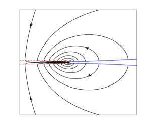
 Figure 4 shows the streamlines of (3.12). The entrainment into the wake in  $r < r_b$ drives a flow that ultimately draws in fluid from the free surface ahead of the fluid bridge in
  $r > r_b$. This flow opens up the gap ahead of the fluid bridge, as we now consider.

Figure 4. Streamlines of the inviscid entrainment-driven flow (3.12).
4. Opening of the gap
From the entrainment-driven streamfunction (3.12) we can calculate the normal velocity  $u_z= r^{-1}\,\partial \varPsi /\partial r$ on the free surface
  $z=0$ for
  $r>r_b(t)$, and thus obtain
 \begin{equation} u_z(r,0;r_b)=\frac{2W}{\rm \pi} \left[ \frac{ r_b }{(r^2-r_b^2)^{1/2}} - \sin^{-1}\frac{r_b}{r} \right]\!. \end{equation}
This velocity is positive for all  $r > r_b$, and therefore, as previously stated, it opens up the gap ahead of the fluid bridge. (From the boundary condition (3.5b), we can also obtain
  $u_r(r,0;r_b)=0$ for
  $r>r_b$.)
The kinematic boundary condition on the free surface is  $\partial h/\partial t=u_z$, where
  $h(r,t)$ is the surface height. By integrating with respect to time, the total increase
  $\Delta h$ in the surface height by time
  $t>0$ at any fixed
  $r>r_b(t)$ is given by
 \begin{equation} \Delta h = \int_0^t u_z(r,0;r_b(t'))\,\mathrm{d} t'. \end{equation}
To evaluate the integral (4.2), we first use (1.1) to change variables, which yields
 \begin{equation} \Delta h(r,r_b) = \frac{2}{D^2} \left(\frac{\rho}{\gamma a} \right)^{1/2} \int_0^{r_b(t)} u_z(r,0;r_b')\,r_b'\,\mathrm{d} r_b'. \end{equation}
We then substitute from (4.1) for  $u_z$, with
  $W$ given by (2.4), and obtain
 \begin{equation} \Delta h(r,r_b) = \frac{12}{{\rm \pi} D^4a} \left[\left(r^2-\frac {2} {3}\,r_b^2\right)\sin^{-1}\frac{ r_b}{r} - r_b(r^2-r_b^2)^{1/2} \right] . \end{equation}
 As  $r_b(t)$ increases towards
  $r$, the entrainment-driven opening of the surface at
  $r$ increases towards the value
 \begin{equation} \Delta h_b (r) \equiv\lim_{r_b \to r_-}\Delta h(r,r_b) = \frac{2r^2 }{ D^4a} . \end{equation}
Thus when  $r_b(t)$ reaches
  $r$, the total surface height
  $h_b$ at
  $r$ is the original surface height
  $r^2/2a$ plus the additional opening (4.5), i.e.
  $h_b(r) = r^2/2a + \Delta h_b(r)$. The additional opening changes the boundary conditions for the leading-order flow in the tightly curved region (within which the gap width closes to zero), with the gap width ahead of this region now given by
  $2 h_b$. This gap width is approximately constant on the radius-of-curvature length scale
  $r_c$, since (4.4) varies on the length scale
  $r_b \gg r_c$.
We determine the rate of coalescence by a volume conservation argument. From § 2, the wake provides the edge of the fluid bridge with volume flux  $Q(r_b)=2\gamma /\rho \dot r_b$ per unit length. We make a simple assumption that the gap ahead of the fluid bridge is filled by this flux. Since the gap of width
  $2 h_b$ needs to be filled at a volumetric rate
  $2 h_b \dot r_b$ (per unit length) for the edge of the fluid bridge to advance at speed
  $\dot r_b$, such a balance implies that
 \begin{equation} \frac{2\gamma}{\rho\dot r_b}= \left(1+ \frac{4 }{ D^4}\right)\frac{ r_b^2 \dot r_b }{a}. \end{equation}
Solving (4.6) for  $D$ with
  $r_b$ of the form (1.1) gives
  $D = 2^{1/2}$. We note that if the effects of entrainment and the additional opening (4.5) were omitted (i.e. if there were no
  $4/D^4$ term), then this argument would give
  $D = 2^{3/4}$.
5. Comparison with previous results
We first compare our prediction for the structure of the flow to the numerical data of AHB. Figure 5 shows that outside the wake on the fluid-bridge scale, the streamlines of the external flow given by (3.12) are in good qualitative agreement with the contours of the Stokes streamfunction (not evenly spaced) given in AHB for  $\textit {Oh} = 0.001$ and
  $r_b = 0.03 a$. Furthermore, near the fluid bridge, the contours of the streamfunction found by AHB are consistent with a thin wake of width
  $\propto (\nu \tau )^{1/2}$, and match a simple calculation of the flow in the wake from vertical diffusion of momentum to give a Gaussian profile. In the wake, the fluid velocity is significantly larger than elsewhere, and it is clear in figure 5(a) that there is indeed entrainment into the wake that is fed by the outer flow.

Figure 5. Numerical and theoretical results for the streamlines (black lines) and surface profile (blue lines) in the case  $\textit {Oh} = 0.001$ for
  $r_b = 0.03 a$. (a) Contours of the Stokes streamfunction (not equally spaced) and the surface profile found numerically by AHB (see their figure 8a). (b) Composite streamlines given by the external streamfunction (3.12) plus, for the flow in the wake, the Gaussian profile produced by vertical diffusion of momentum over the time
  $\tau (r)$ since it was left behind by the advancing edge of the fluid bridge. Curves
  $z = \pm 2 (\nu \tau )^{1/2}$ (red dashed lines) represent a diffusive scaling for the width of the wake. The surface profile includes the opening (4.4).
Figure 6 shows how the surface profile given by the initial profile  $r^2/2a$ plus the additional opening (4.4) for
  $D = 2^{1/2}$ compares to the profile obtained by AHB in the case
  $\textit {Oh} = 0.001$ for
  $r_b = 0.008 a$. There is excellent agreement for
  $r / r_b > 1.05$. The small undershoot of the predicted profile near the tip has only a small volume compared to the total opening due to the entrainment-driven flow, which is consistent with the assumption that the gap ahead of the tip is filled at leading order by the mass provided by the wake. The rounding of the tip on the scale
  $(r-r_b)/r_b =O(r_b/a)$ is to be expected. There is also good agreement for
  $r/r_b>1.2$ with the numerical profile obtained by SS14 for
  $\textit {Oh}=0.01$ and
  $r_b\approx 0.08a$ even though these parameter values are further from the asymptotic limit that we are considering. (SS14 also included a small external viscosity
  $0.006\mu$.)

Figure 6. The theoretical surface profile ahead of the fluid bridge for  $\textit {Oh}\ll 1$ and
  $r\ll r_b$ (dashed red line) obtained by adding the entrainment-driven opening (4.4) for
  $D=2^{1/2}$ to the initial surface profile
  $r^2/2a$ (blue dotted line). Also shown are numerically obtained surface profiles ahead of the fluid bridge for the cases
  $\textit {Oh} = 0.001$ at
  $r_b = 0.008a$ (solid line; see figure 9 of AHB) and
  $\textit {Oh} = 0.01$ at
  $r_b \approx 0.078a$ (short-dashed line; see figure 10 of SS14). The theoretical prediction does not include the rounding of the profile tip on a radial length scale
  $r-r_b=O(r_b^2/a)$, which can be seen in the numerical solutions and in a 1 : 1 plot of the shape (inset).
The theoretical analysis in this paper does not attempt to calculate the detailed flow and interfacial shape on the scale  $r_c\sim r_b^2/a$ of the tightly curved region, and the mechanisms of wake formation, entrainment, external flow and gap opening seen in figure 5 depend not on those details, only on the force
  $2\gamma$. The comparison with the numerical results of AHB, in particular, in figures 5 and 6 provides strong support for the wake-and-entrainment model of the fluid-bridge scale flow that we have derived in this paper.
Figure 7 shows how our theoretically predicted value  $D=2^{1/2}$ for the coefficient of the rate of coalescence (1.1) compares to both the early-time numerical result
  $D=1.5$ of SS14 and the experimental results of PBN. The value
  $D = 1.5$ is only about
  $6\,\%$ larger than
  $2^{1/2}$, which seems reasonably good agreement. The values of
  $D$ that PBN observe experimentally for various fluids with different
  $\textit {Oh}< 0.2$ are in reasonable agreement with
  $2^{1/2}$, given the experimental variations. (We omitted the data for
  $\textit {Oh} >0.2$ as they do not satisfy
  $\textit {Oh} \ll 1$.)

Figure 7. The constant  $D$ for the fluid-bridge radius
  $r_b = D (\gamma a /\rho )^{1/4}t^{1/2}$ in the inertial regime. Experimental results of PBN (dots and error bars) for various Ohnesorge numbers
  $\textit {Oh}$ and the numerical value
  $D=1.5$ from SS14 (dashed line) are shown alongside our theoretically predicted value
  $D= 2^{1/2}$ (blue line) and, for comparison, the value
  $D= 2^{3/4}$ (red line) obtained by omitting entrainment.
6. Discussion and conclusions
We have determined the leading-order flow on the fluid-bridge scale during an inertial regime of early-time drop coalescence. Over the fluid bridge, there is a viscous wake that contains the momentum created by surface tension in the tightly curved region at the edge of the fluid bridge. Fluid is entrained into the wake from above and below, and this entrainment drives an inviscid flow on the fluid-bridge scale that opens up the gap ahead of the fluid bridge. The opening of the gap alters the far-field conditions for the flow at the edge of the fluid bridge, and consequently alters the rate of coalescence.
In the tightly curved region, there is a leading-order force balance between inertia and surface tension that gives the evolution of the fluid-bridge radius as
 \begin{equation} r_b = D \left(\frac{\gamma a }{\rho}\right)^{1/4}t^{1/2}, \end{equation}
where  $D$ is a constant. For a drop with non-zero viscosity, we determined
  $D = 2^{1/2}$ using a volume conservation argument equating the flux provided to the tightly curved region through the wake and the flux used to fill the gap ahead of the fluid bridge. Interestingly, the coefficient
  $D$ does not depend on the viscosity of the fluid in the drop, even though it provides the mechanism for wake formation and entrainment, and the entrainment has a leading-order effect on the value of
  $D$.
$D$.
For  $D = 2^{1/2}$ the streamlines that we obtained for the entrainment-driven flow and the resultant surface profile are in very good agreement with the available numerical data of AHB. In particular, the assumptions made for mass and momentum conservation in the wake and gap are well supported by the numerical results. Moreover, the theoretical value
  $D=2^{1/2}$ that we have obtained is in fairly good agreement with the numerical result
  $D = 1.5$ of SS14, and in reasonable agreement with the experimental results of PBN.
For sufficiently small  $\textit {Oh}$ (at least
  $\textit {Oh} < 0.001$) and sufficiently small external viscosity, it is possible that the dynamics of inertial coalescence might include a series of reconnection events, as calculated for the case of an ideal fluid (
 $\textit {Oh} = 0$) by DEJ. (This has yet to be observed in experiments.) If so, then the flow that we have found on the fluid-bridge scale could also be applied in an average sense to such a case. The momentum created by surface tension between each reconnection event should be left behind with the toroidal bubble in the fluid bridge after each reconnection. (Numerically, DEJ set the existing flow back to zero after each reconnection.) Averaging over many sequential reconnections, this momentum forms a wake with a mass and momentum flux as described in § 2. Then, away from the tightly curved region, there is again an entrainment-driven flow (3.12) that opens up the gap ahead of the fluid bridge. Rescaling the results of DEJ to account for this additional gap opening would reduce the coefficient
  $D$ from approximately
  $1.6$ to
  $1.3$.
Funding
E.B. gratefully acknowledges a UK Engineering and Physical Sciences Research Council studentship (grant no. 2267833).
Declaration of interests
The authors report no conflict of interest.


 Open access