


1. Introduction
Systems involving filament-like structures interacting with fluids are common in nature and many industrial processes, such as microplastics in aquatic environments and pulp production in paper-making (Lundell, Söderberg & Alfredsson Reference Lundell, Söderberg and Alfredsson2011; Guasto, Rusconi & Stocker Reference Guasto, Rusconi and Stocker2012; Du Roure et al. Reference Du Roure, Lindner, Nazockdast and Shelley2019; Carichino, Drumm & Olson Reference Carichino, Drumm and Olson2021), and are studied also due to their similarities with the dynamics of complex systems, such as swimming fish and flapping flags (Zhang et al. Reference Zhang, Childress, Libchaber and Shelley2000; Tian Reference Tian2013). Studies involving Newtonian fluids (Parsa et al. Reference Parsa, Calzavarini, Toschi and Voth2012; Brouzet, Verhille & Le Gal Reference Brouzet, Verhille and Le Gal2014; Ni et al. Reference Ni, Kramel, Ouellette and Voth2015; Allende, Henry & Bec Reference Allende, Henry and Bec2018; Kuperman, Sabban & van Hout Reference Kuperman, Sabban and van Hout2019; Sulaiman et al. Reference Sulaiman, Climent, Delmotte, Fede, Plouraboué and Verhille2019; Żuk et al. Reference Żuk, Słowicka, Ekiel-Jeżewska and Stone2021) are more common compared to the research done on filaments interacting with non-Newtonian viscoelastic fluids. However, filament–fluid interactions in the background of viscoelasticity or ‘polymeric’ influence have gathered more attention recently owing to their presence in many biological and industrial scenarios; to name a few, fluid transport in biological and technological scenarios involving confined environments, such as cilia that transport trapped particles out of the lungs from a viscoelastic mucus layer (Guo & Kanso Reference Guo and Kanso2017), filament-like biological polymers such as actin (Gisler & Weitz Reference Gisler and Weitz1999), pulp fibre suspensions in the paper-making industry (Hearle & Morton Reference Hearle and Morton2008) and in the development of nanocomposite materials wherein the nanotubes (Hobbie et al. Reference Hobbie, Wang, Kim, Lin-Gibson and Grulke2003) are essentially microscopic fibres, suspensions of which can also induce flow-induced gelation and shear thickening (Perazzo et al. Reference Perazzo, Nunes, Guido and Stone2017).
In this work, we study the dynamics of elongated finite-size fibres immersed in a tri-periodic domain forced by a cellular flow, thus dealing with a fibre–fluid viscoelastic system in a highly turbulent flow regime. By ‘finite size’, we mean that the fibre has a finite length, comparable to length scales in the inertial range of turbulence. The presence of polymers introduces also (at least) an additional dimensionless number, called the Deborah number ( $De$), which is the ratio of the polymeric relaxation time scale
  $\varLambda$ over a characteristic time scale of the flow, say
  $L_{0}/U_{rms_{0}}$,
  $L_{0}$ being the integral length scale of the flow, and
  $U_{rms_{0}}$ the root mean square (r.m.s.) flow velocity. Yang & Fauci (Reference Yang and Fauci2017) modelled the motion of a single fibre dispersed in a polymeric cellular flow using two-dimensional computations at very low Reynolds number, and noticed that the fibre in a Newtonian fluid travels faster and buckles earlier in comparison to its viscoelastic counterparts. Often experiments have been carried out to study the dynamics of fibres in polymer-laden flows subject to simple shear flows, where there are interests in probing whether the fibre gets aligned to the vorticity or the flow directions (Iso, Cohen & Koch Reference Iso, Cohen and Koch1996a; Iso, Koch & Cohen Reference Iso, Koch and Cohen1996b); there have been definite industrial interests in knowing how the shear flow orients the semi-flexible nanotubes, and how the elasticity of the viscoelastic melt influences the latter (Hobbie et al. Reference Hobbie, Wang, Kim, Lin-Gibson and Grulke2003). Viscoelastic flows interacting with non-massless deforming structures were studied with an IB-LBM method for the first time by Ma et al. (Reference Ma, Wang, Young, Lai, Sui and Tian2020), who found that viscoelasticity can hinder the three-dimensional flapping motion of flags. Viscoelasticity is also reported to alter the beating patterns of swimmers (filament-like), which in turn influences their swimming velocities and the power dissipated (Fu, Wolgemuth & Powers Reference Fu, Wolgemuth and Powers2008).
The studies mentioned above show irrefutably that the complexities associated with viscoelasticity or non-Newtonian effects are intrinsic to most fibre–fluid interaction systems. However, most of the literature has attempted to test the fibre dynamics under very low Reynolds number flows and two-dimensional flow conditions, which although they can provide clues to the key dynamics, do not unravel the complications arising out of fluid turbulence. In this context, we attempt to track the fibre dynamics for the first time using three-dimensional direct numerical simulations (DNS) in a homogeneous isotropic turbulent viscoelastic flow, to investigate how the polymeric fluid turbulence influences the fibre dynamics, and to analyse if there are qualitative features associated with this system that are not captured by the two-dimensional simplifications in previous studies. Indeed, filament–fluid interactions in past studies conducted in Newtonian turbulent flows have shown that fibre bending stiffness and the linear density difference between the fibre and flow play imperative roles in deciding the fibre's flapping frequency. Oehmke et al. (Reference Oehmke, Bordoloi, Variano and Verhille2021) measured Lagrangian time scales (related to spinning and tumbling) of inertial fibres in turbulence, and reported that they scale with length and diameter of the fibre. It was observed by Rosti et al. (Reference Rosti, Banaei, Brandt and Mazzino2018) and Olivieri, Mazzino & Rosti (Reference Olivieri, Mazzino and Rosti2022) that under the right parametric combinations, the flexible fibres flapped approximately with the turbulent eddy frequency at its length scale, and the stiffer ones flapped with their inherent natural frequency. This observation suggested that fibres could be used to measure the two-point statistics of the flow, at least in certain parametric regimes. It is also in the interests of the present work to understand if viscoelasticity can modify the known dynamics discussed above.
We attempt, for the first time, a systematic approach to study the fully coupled fibre–fluid system at a high Reynolds number turbulent flow, where the fluid is viscoelastic. The simulations are performed for a homogeneous isotropic flow subject to a cellular forcing, with parametric variations in the polymer relaxation time, the fibre's bending stiffness (flexible and rigid fibres), and the linear density difference between fibre and flow (almost neutrally buoyant and denser-than-fluid fibres). The fibre dynamics is tracked through its flapping frequency, the bending curvature, and its alignment with the relevant fluid quantities, to learn if viscoelasticity influences its course of action. The main open question tackled by our study is the following.
(i) What is the dynamical response of a fibre (with rest length in the turbulent inertial range of scales) when it is dispersed in a turbulent viscoelastic flow?
More specifically, we would like to focus on the fibre deformation measured through its end-to-end displacement, and look at various aspects of it, such as the following.
(ii) How does the temporal and frequency dynamics of suspended fibres get influenced in a parametric plane comprising its flexibility, its linear density difference with respect to the fluid, and most importantly, the polymer relaxation time?
(iii) Can one quantify the effects of viscoelasticity on the fibre deformation (e.g. through its curvature and bending energy)?
(iv) Is the alignment of the fibre with the flow (e.g. the principal directions of the strain rate tensor) altered by the presence of polymers?
Section 2 describes the methodology and details of computations carried out to execute the study, § 3 discusses the results, and § 4 concludes the study.
2. Methodology
We consider finite-size flexible fibres with various bending rigidities  $\gamma$ and with lengths
  $c$ within the inertial range of scales, dispersed in a homogeneous isotropic turbulent flow in a cubic domain of size
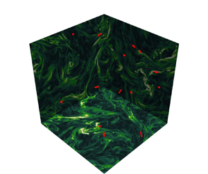
  $L_{d}$ with periodic boundary conditions applied in all directions, as shown in figure 1(a). The reference configuration is chosen such that the Taylor microscale Reynolds number of the corresponding single-phase flow
  ${Re}_{\lambda _{0}} \equiv U_{{rms_{0}}} \lambda _{0} / \nu \approx 310$, where
  $U_{{rms}}$ is the r.m.s. velocity,
  $\lambda _{0}$ is the Taylor microscale, and
  $\nu$ is the kinematic viscosity. In the flow, we inject a series of fibres with different flexibility, achieving a volume fraction
  $\varPhi _{V} = V_{s}/V_{f} = 1.89 \times 10^{-5}$, defined as the ratio of the volume of the dispersed phase
  $V_{s} = Nc{\rm \pi} d^2/4$ to that of the fluid phase
  $V_{f} = L_{d}^3$, where
  $N$ is the number of fibres,
  $d$ is the diameter, and
  $c$ is the unbent fibre length. This implies that the suspension is very dilute and hence the overall back-reaction effects on the flow from the fibre are minimal.

Figure 1. (a) A qualitative snapshot from the DNS simulations for  $Re_{\lambda _{0}} \approx 310$ and Deborah number
  $De \approx 7$, where fibres of various rigidities are dispersed in a tri-periodic domain. The three back planes are coloured based on the trace of the polymer conformation tensor, and the red lines represent the fibres. (b) Schematic of the fibre and the Lagrangian points.
Each fibre is modelled as a homogeneous, inextensible elastic filament evolving according to the Euler–Bernoulli beam equation in a Lagrangian framework:
 \begin{gather} {\rho_{l}} \ddot{\boldsymbol{X}}=\partial_{s}(T\,\partial_{s}(\boldsymbol{X}))-\gamma\, \partial_{s}^{4} \boldsymbol{X}-\boldsymbol{F}, \end{gather}
 \begin{gather} \partial_{s} \boldsymbol{X} \boldsymbol{\cdot} \partial_{s} \boldsymbol{X} =1, \end{gather}
where  $\boldsymbol {X}(s, t)$ is the fibre position based on the curvilinear coordinate
  $s$ at time
  $t$,
$t$,  ${\rho _{l}} = \tilde {\rho }_{{s}} -\tilde {\rho }_{{f}}$ is the difference between the linear densities of the solid and the fluid,
  $\gamma$ is the bending stiffness (defined as the product of the elastic modulus and the second moment of the area),
  $T$ is the tension enforcing the inextensibility, and
  $\boldsymbol {F}$ is the effect of the fluid acting on the fibre. Freely moving boundary conditions are imposed at both fibre ends:
  $\partial _{s s} \boldsymbol {X}|_{s=0, c}=\partial _{s s s} \boldsymbol {X}|_{s=0, c}=T|_{s=0, c}=0$. In this work, we consider both heavy and almost neutrally buoyant fibres, with
  $\rho _{l}=1$ and
  $10^{-3}$, and we vary the bending stiffness over several orders of magnitudes in the range
  $[10^{-8},10^{-2}]$. We can define a non-dimensional bending stiffness
  $\gamma ^{\prime }$ by comparing the inertial and bending terms, i.e.
  $\gamma ^{\prime }$ =
  ${\gamma }/{\rho _{l} U_{rms_{0}}^2 L_{0}^2}$, where
  $L_{0}$ is the integral length scale of the flow, and obtain approximately
  $\gamma ^ {\prime } \in [10^{-8},10^{-1}]$ for neutrally buoyant fibres and
  $\gamma ^ {\prime }\in [10^{-11},10^{-4}]$ for denser ones. These values are comparable to those achieved experimentally by Gay, Favier & Verhille (Reference Gay, Favier and Verhille2018), where
  $\gamma ^{\prime } \in [10^{-6}, 10^{6}]$. A schematic of the fibre is shown in figure 1(b), where
  $x_{1}$,
  $x_{2}$ and
  $x_{3}$ are the coordinate axes corresponding to the Eulerian frame of reference, and
  $nl$ is the number of Lagrangian points on the fibre, taken as 25 here. Suppose that
  $\boldsymbol {X}_{1}$ and
  $\boldsymbol {X}_{2}$ are the Lagrangian coordinates of the fibre tips. Then the end-to-end displacement is defined as
  $\lvert \boldsymbol {X}_{2}- \boldsymbol {X}_{1} \rvert$. In this study, we characterise this quantity, which represents an effective fibre deformation (mainly quantifying its bending).
The fluid flow is governed by the incompressible Navier–Stokes equations for a viscoelastic fluid:
 \begin{gather} \rho\left(\frac{\partial \boldsymbol{u}}{\partial t}+\boldsymbol{u} \boldsymbol{\cdot} \boldsymbol{\nabla} \boldsymbol{u}\right)=-\boldsymbol{\nabla} p+\boldsymbol{\nabla} \boldsymbol{\cdot}\boldsymbol{\tau}+\rho(\,{\boldsymbol{f}_{\!\!fib} +\boldsymbol{f}_{\!\!turb}}), \end{gather}
 \begin{gather} \boldsymbol{\nabla} \boldsymbol{\cdot} \boldsymbol{u}=0, \end{gather}
where  $\boldsymbol {u}(\boldsymbol {x}, t)$ and
  $p(\boldsymbol {x}, t)$ are the velocity and pressure fields,
  $\rho$ is the fluid density,
  $\boldsymbol {\tau }$ is the stress tensor, and
  $\boldsymbol{f}_{\!\!fib}$ is the feedback forcing from the fibre. Here,
  $\,\boldsymbol{f}_{\!\!turb}$ is the external forcing term used to sustain turbulence, chosen to be the Arnold–Beltrami–Childress forcing (Dombre et al. Reference Dombre, Frisch, Greene, Hénon, Mehr and Soward1986) given by
  $\boldsymbol{f}_{\!\!turb}=\nu (A \sin z+C \cos y, B \sin z+A \cos z, C \sin y+B \cos z)$ with constant parameters
  $A = B = C =1$.
The stress tensor  $\boldsymbol {\tau }$ is the sum of two contributions coming from the solvent and polymer (Comminal, Spangenberg & Hattel Reference Comminal, Spangenberg and Hattel2015), i.e.
  $\boldsymbol {\tau }=\boldsymbol {\tau }_{{\!S}}+\boldsymbol {\tau }_{{\!P}}$, with
  $\boldsymbol {\tau }_{{\!S}} =2 \eta _{{s}} \boldsymbol {D}$ and
  $\boldsymbol {\tau }_{{\!P}}=G_0 f_{{S}}(\boldsymbol {c})$, where
  $\eta _{{S}}=\beta \eta _t$ is the solvent viscosity,
  $\beta$ is the solvent to total viscosity ratio, chosen to be equal to 0.9, and the rate of deformation tensor is
  $\boldsymbol {D}=(\boldsymbol {\nabla } \boldsymbol {u}+\boldsymbol {\nabla } \boldsymbol {u}^{\mathrm {T}}) / 2$. Also,
  $G_0=(1-\beta ) \eta _{t} / \varLambda$ is the polymeric elastic modulus,
  $\varLambda$ is the relaxation time, and
  $f_S(\boldsymbol {c})$ is a strain function expressed in terms of the conformation tensor
  $\boldsymbol {c}$, which is representative of the orientation of the polymer chains. A matrix log-conformation formulation (Fattal & Kupferman Reference Fattal and Kupferman2004, Reference Fattal and Kupferman2005; Izbassarov et al. Reference Izbassarov, Rosti, Ardekani, Sarabian, Hormozi, Brandt and Tammisola2018) is used to solve the above equation, where the variable
  $\boldsymbol {\varPsi } = \log \boldsymbol {c}$ is invoked, and the transport equation is modified as
 \begin{equation} \frac{\partial \boldsymbol{\varPsi}}{\partial \boldsymbol{t}}+(\boldsymbol{u} \boldsymbol{\cdot} \boldsymbol{\nabla}) \boldsymbol{\varPsi}-(\boldsymbol{\varOmega} \boldsymbol{\varPsi}-\boldsymbol{\varPsi} \boldsymbol{\varOmega})-2 \boldsymbol{E} =-\frac{1}{\varLambda} \exp (-\boldsymbol{\varPsi})\,f_{{R}}[\exp (\boldsymbol{\varPsi})], \end{equation}
where  $\boldsymbol {\varOmega }$ and
  $\boldsymbol {E}$ are pure rotation (antisymmetric) and pure extension (symmetric traceless) matrices, obtained from the projection of the velocity gradient into the principal base of the stress tensor (Fattal & Kupferman Reference Fattal and Kupferman2004), and
  $f_{R}$ is the relaxation function. In the present work, we consider Oldroyd-B fluids, which have the strain and relaxation functions
  $f_{{S}}(\boldsymbol {c})=f_{{R}}(\boldsymbol {c})=\boldsymbol {c}-\boldsymbol {I}$, where
  $\boldsymbol {I}$ is the identity matrix (Comminal et al. Reference Comminal, Spangenberg and Hattel2015). The conformation tensor
  $\boldsymbol {c}$ is normalised such that at equilibrium, it turns out to be an identity matrix.
The fluid governing equations (2.3)–(2.5) are solved using the fractional step method on a staggered grid, in a domain of length  $L_{d} = 2{\rm \pi}$ that is discretised into a uniform Eulerian grid with
  $500^{3}$ cells, which ensures that the ratio between the Kolmogorov dissipative length scale and the grid spacing is
  $\eta _{0} / \Delta x \approx 0.5$. The adequacy of the grid resolution has also been tested by comparing with results of a
  $1024^{3}$ cell grid in the single-phase flow. The number of Lagrangian points
  $nl$ on the fibre of length
  $c$ is decided such that the spatial resolution
  $\Delta s=c /(nl-1)$ is approximately equal to the Eulerian grid spacing
  $\Delta x$. The in-house-developed solver Fujin (see https://groups.oist.jp/cffu/code) – validated extensively in a variety of problems, including fibres dispersed in turbulent flows (Olivieri et al. Reference Olivieri, Mazzino and Rosti2022) – has been used. The solver is parallelised using MPI and the 2decomp library for domain decomposition. Second-order central finite differencing is used for spatial discretisation, and the Adams–Bashforth scheme for temporal discretisation. Table 1 summarises the values of all the parameters used in the study. We first ran the single-phase configuration without fibres until we obtained a statistically steady state, which was then used to run a non-Newtonian simulation without fibres. Finally, the obtained flow fields were used as initial conditions to run the fibre–fluid cases, where the fibres are released randomly in the domain.
Table 1. Values of parameters used in the study: the domain length  $L_d$, the Taylor-scale Reynolds number
  $Re_{\lambda _{0}}$, the r.m.s. velocity
  $U_{rms_{0}}$, the dissipation rate
  $\epsilon _{0}$, the Kolmogorov length scale
  $\eta _{0}$, and the integral length scale
  $L_{0}$ of single-phase flow, density
  $\rho$ and kinematic viscosity
  $\nu$ of the fluid, the solvent to total viscosity ratio
  $\beta$, the polymer relaxation time
  $\varLambda$, the number of fibres
  $N$, the fibre length
  $c$ and diameter
  $d$, the bending stiffness
  $\gamma$, and linear density difference
  $\rho _{l}$. The range of
  $\gamma$ is spanned in logarithmically equispaced steps.
The mutual interactions between the solid and fluid phases are enforced via singular force distributions acting on the fibre and flow, implemented in the setting of an immersed boundary method (Huang, Shin & Sung Reference Huang, Shin and Sung2007; Rosti et al. Reference Rosti, Banaei, Brandt and Mazzino2018). The material points of the immersed fibre are forced to move with the fluid velocities at those points through a no-slip condition  $\dot {\boldsymbol {X}} = \boldsymbol {u}(\boldsymbol {X}, t)$, where
  $\boldsymbol {X} = \boldsymbol {X}(s, t)$ is the position of a fibre material point, and
  $\boldsymbol {u}=\boldsymbol {u}(\boldsymbol {x}, t)$ is the fluid velocity field. The fluid velocity at the position of the fibre Lagrangian point,
  $\boldsymbol {U}=\boldsymbol {u}(\boldsymbol {X}(s, t), t)$, is obtained by interpolating the fluid velocity at the Eulerian nodes around the Lagrangian point as
 \begin{equation} \boldsymbol{U}(\boldsymbol{X}(s, t), t)=\int \boldsymbol{u}(\boldsymbol{x}, t)\, \delta(\boldsymbol{x}-\boldsymbol{X}(s, t)) \,\mathrm{d}^{3} \boldsymbol{x}, \end{equation}
where  $\delta$ is the Dirac delta function. The interpolated velocity
  $\boldsymbol {U}$ is used to compute the fluid–structure forcing term, represented as
 \begin{equation} \boldsymbol{F}(s, t)=\varUpsilon(\boldsymbol{U}-\dot{\boldsymbol{X}}), \end{equation}
where  $\varUpsilon$ is a large negative constant (Goldstein, Handler & Sirovich Reference Goldstein, Handler and Sirovich1993; Huang et al. Reference Huang, Shin and Sung2007) with value
  $-10$. Finally, the forcing on the fluid from the fibre is calculated as
 \begin{equation} \boldsymbol{f}_{\!\!fib}(\boldsymbol{x}, t)=\frac{1}{\rho} \int_{s} \boldsymbol{F}(s, t)\, \delta(\boldsymbol{x}-\boldsymbol{X}(s, t)) \,\mathrm{d} s . \end{equation}
 In order to examine if there is a spatial inhomogeneity or clustering due to the fibres, the probability density function of the distance between fibres was computed at a low  $De$ and from an instantaneous snapshot. It was seen that the fibres were at a distance of approximately
  $10$ fibre lengths. This implies that the fibres are distributed in a homogeneous manner in the domain owing to their low volume fraction, and the chances of spatial clustering are rare, hence those effects are not considered in further analysis here.
3. Results
3.1. Flow dynamics
We start the analysis by plotting the turbulent kinetic energy  $E$ (normalized with
  $\epsilon _{0}^{2/3} \eta _{0} ^{5/3}$, where
  $\epsilon _{0}$ is the turbulent dissipation rate of the single phase flow), as a function of the wavenumber
  $k/k_{\eta _{0}}$ (
 $k_{\eta _{0}}$ being the wavenumber corresponding to the Kolmogorov length scale defined as
  $2 {\rm \pi}/\eta _{0}$) at three different Deborah numbers,
  $De \approx 0.3, 1, 7$, to identify if viscoelasticity has played a role in bringing deviations to the classical Kolmogorov spectrum, where
  $E(k)\propto k^{p}$ with
  $p=-5/3$, which is the Kolmogorov scaling (K41). It is seen that at the lowest
  $De$ (
 $\approx 0.3$), the spectrum follows the Kolmogorov scaling, as the non-Newtonian effects are weak. As
  $De$ increases to 1, the scaling behaviour is modified: an increasing amount of energy is transferred by the elasticity of the polymers, which alters the spectra to achieve a different scaling coefficient
  $p= -2.3$. Such a scaling behaviour has been elucidated already in non-Newtonian flows without dispersed particles, and has been addressed as an ‘elastic scaling’ in experimental and numerical studies (Zhang et al. Reference Zhang, Bodenschatz, Xu and Xi2021; Rosti, Perlekar & Mitra Reference Rosti, Perlekar and Mitra2023). The range of
  $k$ over which the scaling is valid is called the ‘elastic’ range, and this case turns out to be a clear case of the interaction of elastic and inertial turbulence. This modified scaling does not persist with a further increase in the Deborah number, and the flow recovers the classic Kolmogorov scaling, as shown for
  $De \approx 7$. Thus the spectral character of the fluid shows a non-monotonic trend in the presence of polymers, confirming what has been identified in the literature earlier (Rosti et al. Reference Rosti, Perlekar and Mitra2023). A possible reason for this behaviour is as follows (Singh & Rosti Reference Singh and Rosti2023). The polymeric term
  $({(1-\beta )\eta _{t}}/{\varLambda })\boldsymbol {\nabla } \boldsymbol {\cdot } \boldsymbol {c}$ is close to 0 at low
  $De$, as the polymers stretch minimally and the K41 scaling persists. At
  $De \approx 1$, the time scales of polymer and flow become comparable; additionally,
  $\boldsymbol {\nabla } \boldsymbol {\cdot } \boldsymbol {c}$ also becomes large as the polymers stretch more, hence a multi-scaling spectrum occurs. At higher Deborah numbers, the polymers, with very large relaxation time (
 $\varLambda \rightarrow \infty$), cannot follow the carrier flow, or are rather decoupled from the flow, resulting in a return of the Newtonian scaling. In this study, this behaviour is also present since the flow is dilute, and fibre-induced modulation is negligible. In other words, fibres can be expected to be mere carriers of the information pertaining to the flow, and can possibly be reflective of the polymeric influence in the flow, if any. The inset of figure 2 shows
  $Re_{\lambda }$ (based on the fluid dissipation rate and r.m.s. velocity in the polymeric flow) for each of the three Deborah numbers, which is clearly seen to increase with respect to the single-phase flow (shown with a dotted line), as the fluid dissipation rate drops due to the presence of polymers.

Figure 2. Energy spectra of the turbulent polymeric flows at different Deborah numbers  $De$. The vertical dashed line represents the wavenumber corresponding to the fibre length. The inset shows the resulting Taylor Reynolds number
  $Re_{\lambda }$ for each of the cases.
Following this, we perform a scale-by-scale budget analysis at the intermediate Deborah number  $De \approx 1$ to obtain the flux of kinetic energy
 \begin{equation} \epsilon_{inj}=\epsilon_{f}+\epsilon_{p}=\varPi_{f}(k)+D_{f}(k)+P(k)+\varPi_{fs}(k)+F_{turb}(k). \end{equation}
Here,  $\epsilon _{inj}$ is the total injected dissipation rate,
  $\epsilon _f$ and
  $\epsilon _p$ are the corresponding components from the fluid and the polymer, and
  $\varPi _{f}$,
  $D_{f}$,
  $P$,
$P$,  $\varPi _{fs}$ and
  $F_{turb}$ are the flux contributions from the nonlinear term, viscous term, polymeric stresses, the fluid–structure coupling and the external forcing, respectively. The variation of each of the above flux components (normalised with
  $\epsilon _{inj}$), as a function of wavenumber (normalised with
  $k_{inj}$, the forcing wavenumber) is shown in figure 3(a). An overall observation shows that the contribution from the forcing
  $F_{turb}$ prevails only at the lowest wavenumber, and that the fluid–structure coupling
  $\varPi _{fs}$ is negligible as the volume fraction of the fibres is very low. The nonlinear term
  $\varPi$ dominates at low wavenumbers, taken over by the fluid dissipation
  $D_{f}$ at higher
  $k$ values, which eventually saturates to
  $\epsilon _{f}$. However, at this Deborah number, the effects from the polymer stresses
  $P$ dominate
  $D_{f}$, as one of the effects of polymers is to increase the effective dissipation (Lumley Reference Lumley1973; Hinch Reference Hinch1977; Bird, Armstrong & Hassager Reference Bird, Armstrong and Hassager1987). However,
  $P$ is not a purely dissipative term, which is evident through its non-monotonic behaviour with
  $k$. Rosti et al. (Reference Rosti, Perlekar and Mitra2023) proposed to break down
  $P$ as
 \begin{equation} P(k)=\varPi_{p}(k)+D_{p}(k), \end{equation}
where
 \begin{equation} D_{p}(k)=\frac{\epsilon_{p}}{\epsilon_{f}}\,D_{f}(k). \end{equation}
Here,  $D_{p}$ is a purely dissipative component that saturates to the polymeric dissipation rate
  $\epsilon _{p}$, and
  $\varPi _{p}$ a nonlinear component from the polymer contribution alone. Further, they evaluated the range over which the elastic scaling is valid by simultaneously plotting
  $D_{f}$,
  $\varPi _{f}$ and
  $\varPi _{p}$, which for the present case is shown in figure 3(b). At low
  $k$, the flux is carried predominantly by the solvent
  $\varPi _{f}$, which diminishes as
  $k$ increases, while the polymeric flux
  $\varPi _{p}$ increases. The crossover
  $k$ between these two fluxes is identified as
  $k_{p}$, and the crossover between
  $\varPi _{p}$ and
  $D_{p}$ (or
  $D_{f}$) is defined as
  $k_{\eta '}$, which is the wavenumber when any of the dissipation dominates (Rosti et al. Reference Rosti, Perlekar and Mitra2023). The intermediate range
  $k_{p} < k < k_{\eta '}$ is the elastic range. This exercise has been done in the current context to show that the wavenumber corresponding to the fibre length scale
  $c$, equal to
  $k_{c}/k_{inj} \approx 21$ (corresponding to the dashed vertical line in figures 2 and 3 at
  $k/k_{\eta _{0}} \approx 0.02)$ falls within this elastic regime. In other words, the fibre is in a range of length scales that is dominated by the fluid elasticity.

Figure 3. (a) Flux contributions from (3.1) (normalised with the turbulent energy dissipation rate) plotted with respect to the wavenumber  $k$, at
  $De \approx 1$. (b) The variation of the nonlinear energy flux
  $\varPi _{f}$, fluid dissipation
  $D_{f}$, polymer flux
  $\varPi _{p}$ and polymeric dissipation
  $D_{p}$. The vertical dashed lines represent the wavenumber corresponding to the fibre length.
3.2. Fibre dynamics
3.2.1. Flapping frequency
We now turn our focus to identifying the dominant flapping dynamics of the fibres across different Deborah numbers, primarily by looking at their frequency of flapping. The flapping frequency of fibres interacting with fluids is indeed a well-probed quantity in previous works, due to the interesting transitions that it shows with respect to various parametric variations. Notable mentions in this context are the works by Rosti et al. (Reference Rosti, Olivieri, Banaei, Brandt and Mazzino2020) and Olivieri et al. (Reference Olivieri, Mazzino and Rosti2022), wherein the potential of finite-size flexible fibres to measure relevant two-point statistics of turbulence was highlighted. Mainly, two qualitatively different dynamical regimes were identified: (i) one controlled predominantly by the flow time scales, with the fibres acting as a representative of the turbulent flow; (ii) another controlled by the fibre's natural frequency, in which the effects coming from the carrier flow are negligible. Extending this analysis in the context of a viscoelastic flow scenario for a dilute configuration of dispersed particles is one of the main focuses of this study. We perform a detailed analysis to evaluate the frequency content of the fibre response using a continuous-time wavelet transform and fast Fourier transform on the end-to-end displacement ( $y$) of fibres with different bending rigidities
  $\gamma$, at various Deborah numbers. A goal of this work is to recognise if the fibre at some/all parametric combinations is reflective of changes in the fluid due to the presence of polymers. In this context, it is worth mentioning certain important frequency values associated with the system: (i) the large eddy turnover frequency
  $f_{l} =U_{rms_{0}}/{L_{0}}$, where
  $U_{rms_{0}}$ is the r.m.s. velocity associated with the single-phase flow, and
  $L$ is the integral length scale; (ii) the eddy-frequency at the fibre's length scale
  $f_{c} \approx c^{-2/3} \epsilon ^{1/3}$, where
  $\epsilon$ is the turbulent dissipation rate of kinetic energy, and the formula holds for Newtonian fluids; (iii) the frequency associated with the polymer stretching,
  $f_\varLambda$ =
  $1/\varLambda$; and (iv) the fibre natural frequency (from a normal mode analysis of (2.1)) given by
  $f_{{nat}}=\alpha \sqrt {\gamma /({\rho _{l}} c^{4})}$ (where
  $\alpha \approx 22.4 / {\rm \pi})$.
The time histories of the end-to-end displacement  $y$ normalised with the fibre unbent length
  $c$ are used to explore its frequency behaviours. Note that fast Fourier transforms are useful in capturing the global frequency features of the responses, in contrast to wavelets, which are time–frequency transforms that help to analyse the local characteristics in time. Hence a complementary analysis based on both is useful in the analysis of such highly non-stationary signals, thus such an approach has been used in this work to analyse the flapping frequencies. Figure 4 shows the time histories and their wavelets for two extreme values of rigidities, at
  $\gamma = 10^{-8}$ (flexible, figures 4a,b) and
  $\gamma = 10^{-2}$ (rigid, figures 4c,d). Figures 4(a,c) and 4(b,d) show the cases at two different values of linear densities,
  $\rho _{l}$ =
  $10^{-3}$ and
  ${\rho _{l}} = 1$, respectively. The former represents an approximately ‘neutrally buoyant’ scenario, and the latter corresponds to ‘denser-than-fluid’ fibres; these terms will be used from here onwards. As a starting point, we discuss the flexible fibre in figures 4(a,b). Clearly, the two cases show definite differences: the time histories of neutrally buoyant fibres show rapid variations, fluctuating intermittently between amplitudes as low as
  $0.1$ to amplitudes as high as the fibre's initial length itself (
 $y/c = 1$). On the contrary, the fluctuations are more bounded around similar amplitudes for the denser fibre, with a mean value at approximately
  $0.4$. With respect to the frequency content of the signal, at low
  $\gamma$, it can be seen that the neutrally buoyant responses are dominantly characterised by a broad spectrum of frequencies
  $f/f_{l} \approx 0.05\unicode{x2013}3$ (figure 4a), whereas the denser fibre shows a relatively narrower spread of frequency values around or below
  $f/f_{l} \approx 1$ (figure 4b). Note that frequencies are normalised with the large eddy turnover frequency
  $f_l$.

Figure 4. Time histories and wavelet transform of the fibre end-to-end displacement at the smallest Deborah number  $De \approx 0.3$ for fibres that are (a) neutrally buoyant, flexible (
 $\rho _{l} = 10^{-3}$,
  $\gamma = 10^{-8}$), (b) denser-than-fluid, flexible (
 $\rho _{l} =1$,
  $\gamma = 10^{-8}$), (c) neutrally buoyant, rigid (
 $\rho _{l}=10^{-3}$,
  $\gamma =10^{-2}$), (d) denser-than-fluid, rigid (
 $\rho _{l} = 1$,
  $\gamma = 10^{-2}$).
For the rigid fibre, for neutrally buoyant (figure 4c) and denser (figure 4d) fibres, the time histories convey that the fibre tends to remain in a more unbent configuration, and the frequency behaviours vary drastically across the two linear densities. As the fibre gets more rigid, it starts flapping with higher frequencies; see e.g. figure 4(c), where peaks appear up to  $f/f_{l} \approx 10$. This may be caused by the different shape of the fibre itself. Rigid fibres deform less, or are closer to the initial unbent configuration, and thus can react to small-scale as well as large-scale flow structures around them, resulting in small as well as large time scales in the fibre spectrum. The rigid, denser fibre (figure 4d) shows a band of frequency at
  $f/f_{l} \approx 3$, which corresponds to the natural frequency
  $f_n/f_{l}$ at this
  $\gamma$. The four different cases compared in figure 4 suggest that the flapping dynamics of the fibre (temporal and spectral) is strongly influenced by its density and rigidity: the neutrally buoyant fibres flap with a broader spectrum of fluid time scales, with very large time scales when they are flexible, and a combination of large and smaller time scales as they become more rigid. The denser fibres, however, are limited in their spectrum, with very large time scales related to the flow when they are flexible, or the fibre's natural frequency as they become rigid. The above discussion through wavelets was made to develop an understanding of how the fibre flaps at low Deborah number, close to the classical Newtonian scenario. It is in this picture that we attempt to characterise the effects of polymer elasticity on the flapping dynamics of the fibre in the next part of the paper.
As a next step, we attempt to confirm the existence of this behaviour across different Deborah numbers  $De$ in figure 5: the abscissa represents the frequencies exhibited by the fibre, and the ordinates show their magnitude. Figures 5(a,c,e) and 5(b,d,f) show neutrally buoyant and denser fibres, respectively, and the three rows correspond to Deborah number increasing from top to bottom, with each plot showing the variation in
  $\gamma$s. To plot each of these figures, a wavelet analysis (as shown earlier) was performed first. Then the magnitudes of the wavelet transform of each frequency were averaged in time and subsequently plotted as a function of the frequencies in figure 5. Such an approach has been used to explain and help to visualise the dominant and most relevant frequencies to the system, which are otherwise inherently encapsulated by the variety of time scales and noise introduced by the turbulence. Essentially, we see the same information as in figure 4, but with the temporal effects now averaged out.

Figure 5. Frequency distribution of the fibres from the wavelet analysis, for  $De \approx 0.3, 1, 7$, for (a,c,e) neutrally buoyant fibres (
 $\rho _{l} = 10^{-3}$) and (b,d,f) denser-than-fluid fibres (
 $\rho _{l} = 1$).
We classify the frequencies exhibited by the fibres into two different categories, addressed as low-frequency/large time scale and high-frequency/small time scale regimes, shaded by grey and white regions in figure 5. To visualise specific details of the dynamics, the main plots are represented in a log-linear scale, whereas the insets are shown in a log-log format. The low-frequency regime is due to the large-scale eddies in the flow, while the high-frequency window is from the small-scale eddies or the natural frequency  $f_n$ of the fibre itself. We will show now that the flapping frequency of the fibre is dictated by one of these frequencies in each regime, or a combination of them depending on
  $\gamma$,
  $\rho _{l}$ and
  $De$.
$De$.
First, we examine the dynamics for the neutrally buoyant case (figures 5a,c,e) at all three Deborah numbers. The different colours represent the bending rigidities  $\gamma$, with
  $\gamma \in [10^{-8}, 10^{-2}]$ in steps of
  $10^{-1}$, roughly increasing from top to bottom. The blue dashed vertical line represents the normalised polymeric frequency
  $f_{\varLambda }/f_{l}$. Consistent with the previous observations in figure 4, at the lowest
  $De$ (figure 5a), low-
 $\gamma$ fibres are influenced mainly by the large time scales, with the contribution from the smaller time scales growing as the rigidity increases (see inset). Indeed, at the highest
  $\gamma$ values, high-frequency peaks up to
  $f/f_{l} = 10$ start emerging. Physically, this means that the flexible fibres are controlled mainly by the large-scale structures of the flow, and as the fibre becomes more rigid, it starts being affected also by the smaller eddies around it. At the intermediate
  $De \approx 1$ (figure 5c), the polymeric frequency shifts left as it is an inverse function of
  $De$. We would like to see if there is a difference in the fibre flapping with this change. The main plot shows that there is no spread in frequencies as at the lowest
  $De$: indeed, frequencies are peaking around
  $f/f_{l} \approx 0.4$ and the high frequencies are less evident for the rigid fibres (inset). As
  $De$ is increased further, and
  $f_{\varLambda }$ shifts further leftwards (figure 5e), a significant reduction in the magnitude of the high frequencies can be seen for both low and high
  $\gamma$. Overall, there seems to be a subdominant resonating effect between the excited time scales and the polymeric time scale, resulting in the dominant fibre flapping peaks shifting to smaller values as the polymeric frequency reduces. In other words, the results suggest that an increase in the polymer relaxation time also suppresses the smaller time scales, which are otherwise picked up the fibre. The effects observed in the Lagrangian spectra of the fibre seem to be correlated to what is already known regarding the role of polymers in influencing the turbulent flow structures, i.e. that polymers smooth out small-scale structures and eddies in the flow, and the same effect is transferred to the dynamics of the fibres. Indeed, as the small-scale structures of the flow are damped with increasing
  $De$, the fibres flap with larger time scales.
Next, we discuss the flapping dynamics of the denser-than-fluid fibres in figures 5(b,d,f). The major differences are: (i) compared to the neutrally buoyant case, there is no discernible high-frequency regime at low  $\gamma$ values, and the fibre flaps primarily with the largest time scales of the flow; (ii) as
  $\gamma$ is increased, a singular high-frequency peak is triggered, corresponding to the fibre natural frequency
  $f_n/f_l$, represented by the black circles in the plots. These features are persistent across all the Deborah numbers, indicating a reduced effect of the polymers on the fibre dynamics as they get more inertial.
We show a global picture of the frequencies via the dominant flapping frequencies obtained from a fast Fourier transform of the fluctuation of the end-to-end displacement, plotted as a function of  $\gamma$ in figure 6. Note that we report in the figure results from additional simulations with
  $\gamma =10^{-1}$ and
  $1$ for the denser fibres. In particular, we plot the average of all the frequencies captured by the Fourier analysis that have at least 90 % prominence as the most dominant peak. The black dashed line in the figure corresponds to the large eddy turnover frequency
  $f_l$, while the red dashed line corresponds to the natural frequency
  $f_n$, with all the frequencies being normalised with
  $f_l$. The most important features are: (i) there are flow-driven and fibre-driven flapping regimes; (ii) the denser fibres fall into either of these regimes depending on
  $\gamma$, and show minimum sensitivity with respect to
  $De$; (iii) the neutrally buoyant fibres always fall in the flow-driven regime, but show more sensitivity to the variation in
  $De$. Numerical simulations of rigid fibres moving in laminar flows by Cavaiola, Olivieri & Mazzino (Reference Cavaiola, Olivieri and Mazzino2020) and in turbulent flows by Brizzolara et al. (Reference Brizzolara, Rosti, Olivieri, Brandt, Holzner and Mazzino2021) revealed that as the fibre inertia (linear density) increased, the ability of the fibre to be representative of the flow or to measure two-point flow statistics diminishes. Few analogies on the same lines can be drawn here: the denser fibre sees less changes in the flow when
  $De$ increases, whereas the polymeric fluid flow influences the flapping behaviour of the neutrally buoyant fibres.

Figure 6. The flapping frequency of the fibre from a Fourier analysis, as a function of the bending rigidity  $\gamma$. The inset reports a zoomed view of the same plot in a log-log scale. For dense fibres, we include results from additional simulation with
  $\gamma =10^{-1}$ and
  $1$.
$1$.
3.2.2. Curvature of the fibres
The curvature  $\kappa$ exhibited is another characteristic feature representative of the fibre whose relevance stems from the fact that it is a measure of the flexibility of the body. For example, it was shown experimentally that the extent of flexibility of a filament changes its transport properties in a cellular flow (Wandersman et al. Reference Wandersman, Quennouz, Fermigier, Lindner and Du Roure2010), thus tracking the effects of the relevant control parameters on this observable can possibly be a pathway to identify the overall system dynamics.
We define  $\kappa$ as
  $\sqrt {(x''(s))^2+(y''(s))^2+(z''(s))^2}$, where
  $(x, y, z)$ are the Lagrangian coordinates, and
  $''$ indicates the second derivative with respect to
  $s$. The average of the maximum curvature of each fibre calculated over different Lagrangian points over a few snapshots of time is plotted (dotted lines) in figure 7(a), for both the neutrally buoyant fibres (open circles) and the denser case (closed circles). Also, the average of the mean curvature is represented (solid lines) for neutrally buoyant fibres (open squares) and the denser case (closed squares). The denser-than-fluid fibres show a higher curvature compared to the neutrally buoyant case, a consequence of the former being more inertial. This can be interpreted by balancing inertial forces
  ${\rho _{l}} \ddot {\boldsymbol {X}}$ and bending forces
  $\gamma \,\partial _{s}^{4} \boldsymbol {X}$;
  $\partial _{s}^{2} \boldsymbol {X}$ being the curvature, it can be seen that as
  $\rho _{l}$ increases, the curvature can indeed increase for the same
  $\gamma$. The curvature
  $\kappa$ decreases with increasing stiffness
  $\gamma$, being almost constant with high values for flexible fibres, transitioning into lower values for highly stiff fibres through an intermediate regime with interim values. The variation of the curvature with
  $De$ shows a non-monotonic trend at the intermediate
  $De$ in the neutrally buoyant scenario. The elastic energy stored by the fibres defined as
  $E_{el} = \int _0^c \tfrac {1}{2} \gamma \kappa ^2\,{\rm d}s$ is plotted in figure 7(b). The denser fibres have higher elastic energy, consistent with their overall larger curvature, but seem to be unaffected by
  $De$, whereas an evident drop is exhibited by the neutrally buoyant fibres as
  $De$ changes from 0.3 (low) to 1 (interim), which recovers when
  $De$ is increased further.

Figure 7. (a) Curvature and (b) elastic energy stored by the neutrally buoyant and denser fibres at various  $De$. Open and closed symbols are used to distinguish neutrally buoyant and denser cases, respectively, while in (a), we use dotted and solid lines to distinguish the maximum and mean curvatures.
To better perceive how the fibre shape deforms, we further probe into the fibre curvature by plotting in figure 8(a) temporally averaged  $\kappa$ of each fibre as a function of its normalised length
  $s/c$. Figures 8(a,c,e) and 8(b,d,f) respectively show the neutrally buoyant and denser cases, with figures 8(a,b), 8(c,d) and 8(e,f) representing
  $De \approx 0.3$, 1 and 7, respectively. Clearly, as rigidity increases,
  $\kappa$ decreases for all cases. For the highest
  $\gamma$, the neutrally buoyant fibres are almost in an unbent configuration in comparison with the denser ones at the highest
  $\gamma$ (compare the abscissa of figures 8a,b), which exhibits a unimodal shape. The denser fibre further becomes bimodal and multimodal from thereon as
  $\gamma$ decreases, eventually becoming a highly flexible and deformable body. This happens also for the neutrally buoyant fibres, but at much lower
  $\gamma$; indeed, for the same rigidity, the deformation and magnitudes of the neutrally buoyant fibres are lower compared to the denser ones.

Figure 8. The curvature  $\kappa$ plotted as a function of the normalised length
  $s/c$, along the fibre length at (a,b)
  $De \approx 0.3$, (c,d)
  $De \approx 1$, and (e,f)
  $De \approx 7$, for (a,c,e) neutrally buoyant and (b,d,f) denser cases.
Figures 8(a,b) ascertain that for the same stiffness, fibres of higher linear density buckle to a higher extent in comparison to the neutrally buoyant ones (see the green colours). In other words, a dynamical transition to buckling from an unbent configuration is easily initiated when the fibres are more inertial. When investigating if viscoelasticity further hinders this behaviour, we observe that the deformations of the neutrally buoyant fibres (figures 8a,c,e) are slightly affected by viscoelasticity, while the denser fibres are insensitive to variations in fluid elasticity (figures 8b,d,f). It is known that capsules in an Oldroyd-B shear flow experience monotonically decreasing or increasing deformations depending on the level of elasticity, and that the three-dimensional flapping of a flag is hindered by viscoelasticity (Ma et al. Reference Ma, Wang, Young, Lai, Sui and Tian2020). Fu et al. (Reference Fu, Wolgemuth and Powers2008) defined a bending scale for filament-like swimmers (higher for stiff filaments, and smaller for flexible filaments deforming due to fluid forces), and reported that viscoelasticity increased this bending scale. This was correlated to the beating patterns of swimmers changing from travelling waves to standing waves as Deborah number increased. All these studies were conducted at lower Reynolds numbers, where the fluid turbulence was not relevant, whereas the present study extends this understanding to turbulent scenarios in a broader parametric setting. Scrutinising the effects of viscoelasticity on the filament deformations along similar lines as the above-discussed studies leads one to conclude that increased polymer stretching can influence the fibre curvature quantitatively, but does not impact it qualitatively.
3.2.3. Alignment
We now try to understand whether there is a preferential alignment of the fibre towards specific flow quantities such as the principal direction of strain rate or that of the conformation tensor. In turbulent mixing, it is of interest usually to understand how material fluid elements orient with components of velocity gradient tensor (Guala et al. Reference Guala, Liberzon, Lüthi, Kinzelbach and Tsinober2006). Flow-induced fibre alignment has a significant influence on the properties of composite materials, such as those made by processes like injection molding. This property is also highly dependent on the configuration: e.g. in homogeneous isotropic turbulence flows, fibres are known to usually align with the intermediate eigenvector of the strain rate tensor, whereas for channels, they are a function of the channel height, largely influenced by the coherent structures (Cui et al. Reference Cui, Huang, Xu, Andersson and Zhao2021). Clearly, the alignment can also be influenced by viscoelastic stresses; experiments with low Reynolds number simple shear flows have shown that orientation of semi-dilute fibre suspensions in weakly (Iso, Koch & Cohen Reference Iso, Koch and Cohen1996b) and highly (Iso et al. Reference Iso, Cohen and Koch1996a) elastic fluids change in comparison to their aligned directions in Newtonian flows (Stover, Koch & Cohen Reference Stover, Koch and Cohen1992). Further, this trend itself showed a complex set of behaviours based on the fibre concentration (Iso et al. Reference Iso, Cohen and Koch1996a,Reference Iso, Koch and Cohenb).
The fibre's local orientation (considering segments connecting two Lagrangian points) with the local fluid flow is computed instantaneously, and after adopting a coarse-graining procedure, the existence of a preferential alignment with any of the principal directions ( $\hat {e}_{i}$) of the strain rate and of the conformation tensor are explored. The three principal directions are chosen as
  $i_{min}, i_{inter}, i_{max}$ corresponding to eigenvalues
  $\chi$ such that
  $\chi _{min}<\chi _{inter}<\chi _{max}$, respectively. Usually, the eigendirection corresponding to
  $\chi _{max}$ corresponds to the most extensional direction, and
  $\chi _{min}$ corresponds to the eigenvalue of the least extensional direction.
In figure 9, we consider only the neutrally buoyant fibres and show the alignment of the fibre's orientation with the strain rate principal directions (figures 9a,c,e) and with the conformation tensor principal directions (figures 9b,d,f) at  $De \approx 0.3, 1, 7$ (top to bottom). The solid, dashed and dotted lines correspond to
  $i_{min}$,
  $i_{inter}$ and
  $i_{max}$, respectively. Two extreme values of
  $\gamma$ are chosen, corresponding to flexible (
 $\gamma = 10^{-8}$, red) and rigid (
 $\gamma = 10^{-2}$, green) fibres. It can be seen that for all three Deborah numbers, the fibres are mainly aligned with the intermediate eigenvectors (
 $i_{inter}$) of the strain rate, and with the most extensional direction (
 $i_{max}$) of the conformation tensor. The anti-alignment with the least extensional direction (
 $i_{min}$) persists instead in both cases. It is also interesting to note that the variations of these trends for flexible and rigid fibres are negligible. Statistics of alignment of neutrally buoyant slender, microscopic fibres in homogeneous isotropic Newtonian flows (Pumir & Wilkinson Reference Pumir and Wilkinson2011; Ni et al. Reference Ni, Kramel, Ouellette and Voth2015) showed a tendency to align with
  ${i}_{inter}$, to be mostly perpendicular to
  ${i}_{min}$, and have no particular alignment with
  ${i}_{max}$, in agreement to figures 9(a,c,e) here. Despite that, in polymeric flows the fibres are seen to align more with the most extensional direction of the polymeric tensor.

Figure 9. Probability density functions (p.d.f.s) of the alignment of neutrally buoyant fibres with the principal directions of (a,c,e) the strain rate tensor and (b,d,f) the conformation tensor, at (a,b)  $De \approx 1$, (c,d)
  $De \approx 3$, and (e,f)
  $De \approx 7$. Solid, dashed and dotted lines correspond to
  $i_{min}$,
  $i_{inter}$ and
  $i_{max}$, respectively.
Major differences observed in the alignment of the denser-than-fluid fibres (figure 10) are that (i) the flexible and rigid fibres behave differently, and (ii) the alignment of the fibres with the polymeric tensor principal directions changes with the Deborah number, although with lower probabilities compared to their alignment with the velocity gradient tensor. At  $De \approx 0.3$ (figure 10a), the fibre is still aligned with the intermediate eigenvector of the strain tensor, but it is anti-aligned with the most and least extensional directions. This alignment and anti-alignment trend is modified with the conformation tensor (figure 10b), where the fibre is anti-aligned with the intermediate direction and aligned with the least and most extended directions. This behaviour is visible only for the most rigid fibres, while the flexible ones are nearly uniformly distributed, indicating no preferential direction. Further, as
  $De$ increases, the trends with respect to the strain rate matrix hold similar to the previous case (figures 10c,e), while with the conformation tensor we see a change: the alignment of the rigid fibres with the most extended direction vanishes at
  $De \approx 1$ (figure 10d), and returns at the larger value of
  $De$ (figure 10f). In short, the preferential alignment of the denser-than-fluid fibres is a function of the rigidity as well as the Deborah number. Also, consistently with the previous observations of this study, they do not quite follow the polymeric extensional direction of the neutrally buoyant fibres.

Figure 10. Probability density functions of the alignment of denser-than-fluid fibres with the principal directions of (a,c,e) the strain rate tensor and (b,d,f) the conformation tensor, at (a,b)  $De \approx 1$, (c,d)
  $De \approx 3$, and (e,f)
  $De \approx 7$. Solid, dashed and dotted lines correspond to
  $i_{min}$,
  $i_{inter}$ and
  $i_{max}$, respectively.
Dotto & Marchioli (Reference Dotto and Marchioli2019) investigated the orientation of inertial flexible fibres in channel flow, for different lengths and Stokes numbers of the fibre. Although a function of the channel height, it was reported that the fibre mean orientations in the streamwise and wall-normal directions showed a lesser tendency to align preferentially with the flow as the fibre inertia increased. The authors also mention that the fibre flexibility plays only a secondary role when fibre inertia is large enough. Analogously, here we also observe that an increase in fibre inertia influences the alignment of fibres, and that flexible fibres show no preferential alignment.
3.2.4. Preferential sampling
Finally, we investigate the preferential sampling of fibres. To do so, we compare the trace of the conformation tensor around the fibres (measured in a Lagrangian way) and that in the whole domain (measured in an Eulerian way). Note that the trace is a direct quantifier of the extension of the polymers, and the objective here is to find out to what extent the fibres see the polymer stretching. Figure 11(a) shows the trace of the conformation tensor experienced by the fibres for the three different values of  $De$, at a fixed value
  $\gamma = 10^{-8}$. The black curves correspond instead to the Eulerian data. Both shift towards the right to higher values with increasing Deborah number, a direct effect of the increasing polymer extension with
  $De$. The probability density functions of the trace of the conformation tensor in the domain exhibit a very wide distribution at all
  $De$, positively skewed. The Lagrangian distributions show a similar shape, but with larger mean values and reduced tails; thus fibres do not sample the whole regions of maximum polymer stretching. Denser fibres tend to sample more regions of high polymer extension at low
  $De$, while the opposite is evident at larger Deborah numbers. Figures 11(b,c) show the means and standard deviations of the neutrally buoyant and denser fibres, respectively. Evidently, there is not much effect on the stiffness of the fibre, whereas the rate of increase in trace with respect to
  $De$ is slightly higher for the neutrally buoyant fibres. Nevertheless, the fibres not sampling the regions with extreme polymer stretching can be the reason for the moderate effect of the Deborah number on their dynamics.

Figure 11. (a) Probability density function of the trace of the conformation tensor (black) measured in the whole domain and (colours) perceived by the fibres, i.e. measured in a Lagrangian way. Dashed and dotted lines correspond to the neutrally buoyant and denser fibres, both at  $\gamma = 10^{-8}$. (b,c) Mean and standard deviation of the probability density function of the trace of the conformation tensor for (b) neutrally buoyant and (c) denser fibres. The black lines represent the mean values of the Eulerian data.
4. Conclusions
We perform direct numerical simulations (DNS) to explore the dynamical properties of fibres (both flexible and rigid, neutrally buoyant and denser-than-fluid fibres) dispersed in a viscoelastic turbulent flow where fluid inertia and polymer elasticity are present simultaneously, with the three phases – fluid, polymers and fibres – which are fully coupled. The Reynolds number is sufficiently high to show a clear inertial range of scale, which is altered when the Deborah number is increased. The goal is to examine how the microscopic polymers can influence the dynamics of macroscopic fibres, and to identify if the fibres reflect the changes in the fluid due to the polymers. For this, the flapping frequency of the fibres, their curvature, preferential alignment with and sampling of the flow were tracked for various values of the Deborah number.
We observe that the fibres flap primarily with a variety of time scales, transpiring from the flow or their structural natural response, depending on the particle inertia, stiffness, and the polymer relaxation time. An examination of the frequency spectrum of the end-to-end displacement of the fibres showed that the expected time scale due to polymer stretching is not picked up explicitly by the fibre. Still, the neutrally buoyant fibres are weakly reflective of the polymer effects as the dominant flapping time scales of the fibre are also seen to increase with the polymer relaxation time; on the other hand, the denser-than-fluid fibres always oscillate with large time scales when flexible, and with their natural frequency when sufficiently rigid, irrespective of the changes in the Deborah number. Polymer relaxation time impacts the neutrally buoyant fibre curvature quantitatively, but does not significantly impact the transition to buckling; on the contrary, the denser fibres – which also exhibit larger curvatures – are passive to the variations of the relaxation time. The neutrally buoyant fibres show a high level of alignment with the polymer conformation tensor, unresponsive to variations in their rigidity and the Deborah number. Conversely, the alignment of the denser fibres changes with both the Deborah number and the rigidity, especially with respect to the polymeric tensor, although these probabilities are much lower than the corresponding alignment with the strain rate tensor.
This study attempts for the first time to track the dynamical properties of long fibres fully coupled with viscoelastic high Reynolds number turbulent flows. It reveals a complex interplay between the fibre flexibility, the polymer relaxation time, and the fibre inertia in determining the response behaviours of the fibres. The study can be of interest to industries developing products/processes involving viscoelastic fluid–fibre suspensions to optimise manufacturing and quality control processes, and is a fundamental addition to this field of study. Future works should take into account the effect of gravity as well. Ardekani et al. (Reference Ardekani, Sardina, Brandt, Karp-Boss, Bearon and Variano2017) studied the sedimentation of prolate spheroids in homogeneous isotropic turbulence with application to non-motile phytoplanktons, and showed that settling spheroids showed an increased mean settling speed from those in a quiescent fluid; the authors of this study suggest that flexural stiffness is a dynamically important attribute to diatom chains that should be taken into account in future studies. Also, the ability of shear thinning fluid to modify particle sedimenting velocity has been demonstrated by Alghalibi et al. (Reference Alghalibi, Fornari, Rosti and Brandt2020) through DNS. Along similar lines, it would be compelling to track the observations made in the current work by considering sedimentation effects along with considering fibre stiffness and Deborah number effects. Banaei et al. (Reference Banaei, Rahmani, Martinez and Brandt2020) found definite differences between rigid and flexible fibres with respect to their settling velocities and alignment with the direction of gravity, while Rahmani et al. (Reference Rahmani, Banaei, Brandt and Martinez2023) described the shapes of inertial settling flexible fibres of large aspect ratios. It would be intriguing to perceive these known dynamics of sedimenting fibres in the background of elasto-inertial turbulence.
Funding
The research was supported by the Okinawa Institute of Science and Technology Graduate University (OIST) with subsidy funding from the Cabinet Office, Government of Japan. The authors acknowledge the computer time provided by the Scientific Computing section of Research Support Division at OIST and the computational time provided by the High Performance Computing Infrastructure (HPCI) under the grants hp210025, hp220099.
Declaration of interests
The authors report no conflict of interest.


 Open access