


Abstract
Active regions are the brightest structures seen in the solar corona, so their physical properties hold important clues to the physical mechanisms underlying coronal heating. In this work, we present a comprehensive study for a filament-embedding active region as determined from observations from multiple facilities including the Chinese Hα Solar Explorer. We find three types of dynamic features that correspond to different thermal and magnetic properties, i.e., the overlying loops—1 MK cool loops, the moss region—2–3 MK hot loops' footprints, and the sigmoidal filament. The overlying cool loops, which have a potential field, always show Doppler blueshifts at the east footprint and Doppler redshifts at the west, indicating a pattern of "siphon flow." The moss-brightening regions, which sustain the hot loops that have a moderate sheared field, always show downward Doppler redshifts at the chromosphere, which could be a signature of plasma condensing into the inner region adjacent to the filament. The sigmoidal filament, which has strongly sheared field lines along the polarity inversion line, however, shows a different Doppler velocity pattern in its middle part, i.e., an upward Doppler blueshift at the double-J-shaped stage indicating tether-cutting reconnection during the filament channel formation and then a downward redshift showing the plasma condensation for the sigmoidal filament formation. The present work shows overall properties of the filament-embedding active region, constraining the heating mechanisms of different parts of the active region and providing hints regarding the mass loading of the embedded filament.
Export citation and abstract BibTeX RIS

Original content from this work may be used under the terms of the Creative Commons Attribution 4.0 licence. Any further distribution of this work must maintain attribution to the author(s) and the title of the work, journal citation and DOI.
1. Introduction
Active regions are the fundamental structures at the solar surface, and investigation of their overall properties, such as their emission measure, magnetic field, and dynamics will be helpful for understanding the coronal heating problem. It is generally believed that there are different types of coronal loops in an active region. The cool loops, which are rooted at the magnetic concentrations, are well identified in 173 Å of the Transition Region and Coronal Explorer (Handy et al. 1999) and 171 Å of the Solar and Heliospheric Observatory/Extreme-Ultraviolet Imaging Telescope (Delaboudinière et al. 1995) and have been identified as 1 MK loops (Del Zanna & Mason 2003; Del Zanna 2003). The hot loops, which were initially identified in soft X-ray (SXR) images, have the footprints rooted in the brightening-moss region (Berger et al. 1999; Martens et al. 2000). Two different mechanisms of heating have been proposed according to the Doppler velocity of the active region, i.e., the steady heating and the impulsive heating. Both evidences of steady heating (Antiochos et al. 2003; Schrijver et al. 2004; Brooks & Warren 2009; Warren et al. 2010) at the footprints, as well as impulsive heating and condensing high above, (Tripathi et al. 2010) have been found for the hot loops. The 1 MK extreme-ultraviolet (EUV) loops, however, are more dynamic and are considered to be impulsively heated to high temperatures and then cooled down (Aschwanden et al. 2001; Warren et al. 2002; Winebarger & Warren 2005; Landi et al. 2009; Viall & Klimchuk 2011, 2012) although observation also shows the SXR loops and EUV 171 and 195 Å loops are independent phenomena and are generated by different processes (Schmieder et al. 2004).
The correspondence of the active-region structures observed in chromospheric lines and the transition region lines has been identified (De Pontieu et al. 2003), yet previous works (Brooks & Warren 2009; Tripathi et al. 2012; Winebarger et al. 2013; Ghosh et al. 2017) mainly focus on the transition region and corona observations with the Solar Ultraviolet Measurement of Emitted Radiation (Wilhelm et al. 1995) on board the Solar and Heliospheric Observatory (Domingo et al. 1995), EUV Imaging Spectrometer (Culhane et al. 2007) on board Hinode (Kosugi et al. 2007), and Interface Region Imaging Spectrometer (IRIS; De Pontieu et al. 2014). As the heating process could happen in the lower atmosphere rather than in the corona (Aschwanden et al. 2007), the chromospheric Doppler velocity, which has rarely been studied for the active region, will provide some constraints on the heating mechanisms of the active-region loops.
Most prevalently, solar filaments, which are manifestations of cool plasma suspended in the hot solar atmosphere, could form in the active region, being adjacent to the brightening-moss region. It is generally believed that the filament is sustained in the magnetic dips of sheared arcades or magnetic flux ropes and their eruptive counterparts include the whole body of the flux rope, which is much larger than the space occupied by the filament, namely, the entire filament channel.
The filament itself has been the subject of intensively focused studies (see Chen et al. 2020 and references therein), while the filament channel has rarely been studied due to the faint signals in the atmosphere. One of the most intriguing questions is how the filament channel as well as the filament forms. Three models have been proposed and supported by the observations. The evaporation-condensation model is triggered by the heating around the footprints of the loops, while the condensation is the main result of radiative losses associated with thermal nonequilibrium (Liu et al. 2012; Xia et al. 2014; Xia & Keppens 2016; Li et al. 2021; Yang et al. 2021). The levitation model suggests that the cool plasma of the filament is lifted during the emergence of the helical magnetic structure or during the cancellation of the magnetic field near the polarity inversion line (PIL), which is more likely for filaments in active regions (Yardley et al. 2019; Baker et al. 2022). The injection model is proposed based on the observation of prominence plasma fed by jet events (Chae 2003; Wang et al. 2018), and it is highly associated with the reconnection process that is crucial for the filament-channel formation (van Ballegooijen & Martens 1989; Wang & Muglach 2007).
The magnetic structure of filaments including quadrupolar magnetic arcades (Moschou et al. 2015), or twisted flux ropes (Xia & Keppens 2016; Fan & Liu 2019), are frequently simulated. Basically, an evaporation-condensation process is obtained in most simulations, while levitation-condensation is derived for an emerging flux rope (Fan & Liu 2019; Jenkins & Keppens 2021). Whether there is a general scenario for the formation of filament channels as well as filaments remains unclear.
In the present work, a filament-embedding active region, which has been observed intermittently for 48 hr with spectral information ranging from the chromosphere to the transition region, is investigated. The paper is organized as follows: we show the observations in Section 2. The thermal properties, 3D magnetic field distribution, and spectral analysis are shown in Sections 3, 4, and 5, respectively. We give our discussion and conclusion in Section 6.
2. Observations
During 2022 February 14–17, NOAA Active Region (AR) 12946 has been observed in its passage across the solar disk with multiple instruments, and a typical sigmoidal filament has been formed and erupted. The entire process was observed by the Atmospheric Imaging Assembly (AIA; Lemen et al. 2012) and Helioseismic and Magnetic Imager (HMI; Schou et al. 2012) on board the Solar Dynamics Observatory (SDO; Pesnell et al. 2012) synoptically. The evolution of the filament during its preeruptive phase was also captured by the facilities of the New Vacuum Solar Telescope (NVST; Liu et al. 2014), the Chinese Hα Solar Explorer (CHASE; Li et al. 2022a), and the IRIS (De Pontieu et al. 2014) with high resolution. Fields of view (FOVs) of the different instruments or analyses that are shown in Sections 3–5 are displayed in the top panel of Figure 1. Such selections enable each studied structure to be displayed around the center of the FOV. As the activities in the active region have been observed intermittently by different instruments except SDO, the overall time coverage is displayed in the bottom panel of Figure 1.

Figure 1. Different FOVs are displayed in the top panel for the following demonstrations: DEM analysis (green box), CHASE Doppler velocity analysis (blue box), NVST observations (red box), DAVE4VM analysis (purple box), and IRIS observations (white rectangle). The background is AIA/171 Å image on 2022 February 15. Time coverage of observations from NVST (green), CHASE (pink), and IRIS (blue) on 2022 February 14–15 is displayed in the bottom panel.
Download figure:
Standard image High-resolution imageFrom the photosphere to corona, AR 12946 was observed by SDO/AIA in seven EUV and three ultraviolet (UV)/visible wavelengths, covering a temperature range of 0.005–20 MK. The alignment of AIA images with the images at Hα line center from other instruments is achieved through the UV image in 304 Å.
The filament was intermittently observed by NVST between 2022 February 13 and 16, capturing the transformation from two J-shaped segments to a sigmoidal filament. The images are sampled at Hα line center and line wings of ±0.6 Å. The temporal resolution is around 12 s, and the pixel size is as high as 0 165.
165.
The Hα imaging spectrograph (HIS) on board CHASE implements raster scanning of the full solar disk for the first time. It scans an FOV of  ×
× in 60 s in the wave bands of Hα and Fe i with pixel spectral resolution as high as 0.024 Å and pixel size of 0''52. The observation duration on 2022 February 14 is around 20 minutes from 07:24 UT to 07:41 UT, and on February 15, it is around 2 hr from 10:15 UT to 12:15 UT. With the full-disk scanning data, the overall kinetic features of the active region were obtained at the chromosphere. One may notice that the spatial resolution of CHASE/HIS was greatly improved after in-orbit calibration since 2022 August 4. The present data show the large-scale dynamic features of the active region.
With a limited FOV, the middle part of the filament, where the reconnection might happen, was also observed by IRIS with a sit-and-stare mode during February 14 and with a step raster mode during February 15 and 16. It was observed in Mg ii h and k lines ( ), C ii (
 ), Si iv (
 ), and Fe xii (
 ). The Doppler velocity at the upper chromosphere was obtained through the Mg ii h line, while the optical property of the filament was derived through the line ratio of the Si iv line pair (Mathioudakis et al. 1999).
3. Thermal Properties
AR 12946 has been observed by SDO/AIA with multiple EUV wavelengths, and differential emission measure (DEM) analysis (Weber et al. 2004) is carried out for obtaining the thermal property. The latest version of the revised Sparse DEM code (Cheung et al. 2015; Su et al. 2018) has been adopted. A binning of 3 × 3 pixels is used to increase the signal-to-noise ratio, and a temperature bin size of  on the same order of the AIA temperature response capability is used. The calculation covers a temperature range of [5.5, 7.6] K in logarithmic scale. The results of emission measure at different temperatures for the sigmoidal filament stage are displayed in Figure 2. The top panels show the intensity images of AIA 171 Å (Fe ix, 0.9 MK), 193 Å (Fe xii, 1.5 MK), and 335 Å (Fe xvi, 2.5 MK) for AR 12946. The middle panels show the emission measures from 0.7 to 0.9 MK, which are dominated by the external part of the active region. The bottom panels show the emission measures from 2.5 to 3.2 MK, which are dominated by the core part of active region. The core part of the active region also has emission measures at lower temperatures and some emission measures at higher temperatures, which are not displayed here.
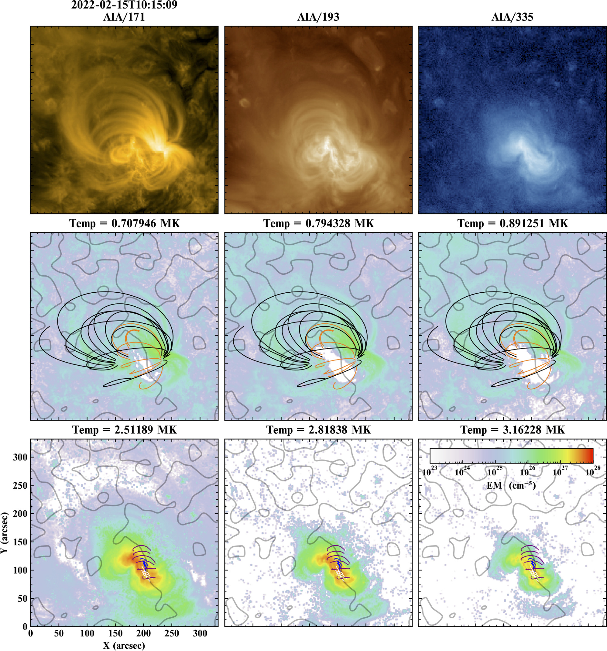
Figure 2. Overview of AR 12946 on 2022 February 15. Intensity images of AIA/171, 193, 335 Å are displayed in the top panels. Emission measures at different temperature ranges, i.e., 0.7–0.9 MK and 2.5–3.2 MK, are displayed in middle panels and bottom panels, respectively. Three-dimensional magnetic field lines of different systems are overlaid at the emission measure plots. The gray contours with a value of 0 G are from the Gaussian-smoothed magnetogram to show the PIL.
Download figure:
Standard image High-resolution image4. Three-dimensional Magnetic Field
The 3D magnetic fields at the sigmoidal filament stage of AR 12946 have been reconstructed through a nonlinear force-free field (NLFFF) extrapolation based on the open source Message-Passing Interface-Adaptive Mesh Refinement Versatile Advection Code, or MPI-AMRVAC, software (Keppens et al. 2003; Xia et al. 2018; Keppens et al. 2023). To perform this extrapolation and ensure that the FOV covers coronal loops, we extracted the required photospheric boundaries from the full-disk vector magnetic field of the SDO/HMI "hmi.B_720s" series. Generally, the "bvec2cea.pro" routine in the SolarSoft HMI package is adopted. It can easily handle three aspects of the "hmi.B_720s" series (Sun 2013; Hoeksema et al. 2014a), including the 180° disambiguation for the transverse field, remapping from the CCD coordinates to the heliographic cylindrical equal-area (CEA) coordinates with a spatial sampling of 0 03 (∼0.36 Mm) per pixel, and conversion of the vector magnetic field components at each coordinate point into the description of (Br
, Bt
, Bp
) through vector transformation. The components (Bp
, − Bt
, Br
) are usually treated as (Bx
, By
, Bz
) for extrapolation in Cartesian coordinates. Finally, a region of 500 × 452 pixels2 considering flux balance is cropped out and preprocessed as the boundary condition for the NLFFF extrapolation.
03 (∼0.36 Mm) per pixel, and conversion of the vector magnetic field components at each coordinate point into the description of (Br
, Bt
, Bp
) through vector transformation. The components (Bp
, − Bt
, Br
) are usually treated as (Bx
, By
, Bz
) for extrapolation in Cartesian coordinates. Finally, a region of 500 × 452 pixels2 considering flux balance is cropped out and preprocessed as the boundary condition for the NLFFF extrapolation.
Magnetic field lines that represent different emission systems are displayed in Figure 2. The external high loops (black and orange lines) correspond well to the ∼1 MK emission measures, while the inner low loops (dark purple lines) rooted at the core region represent the 2–3 MK hot loops. The field lines corresponding to the sigmoidal filament are also displayed in white and blue although the emission measure does not have any information of the filament structure. Referring to the PIL, the distribution of the magnetic field lines shows a potential morphology for the ∼1 MK loops, while the 2–3 MK hot loops correspond to moderately sheared arcades. The sigmoidal filament, however, corresponds to severely sheared arcades along the PIL.
5. Plasma Dynamics
The spectral analysis has been carried out for Hα and Mg ii lines, obtaining Doppler velocity from the low to the upper chromosphere. The analysis of the complex Mg ii line refers to the iris_get_mg_features_lev2.pro in the IRIS analysis guide.
5.1. Overall Structures
The Doppler velocity of the entire active region at the chromosphere was obtained for the spectrum of the Hα line by fitting the observed line profile within ±0.5 Å with a Gaussian. The reference line center was calculated in a quiet square region near the disk center. There are several other ways (see Qiu et al. 2024 and references therein) to obtain the Doppler shift of Hα lines, and two general methods, i.e., the moment analysis and the bisector method, are adopted and confirm the Doppler velocity obtained here. The first one is to calculate the line core weighted-averaged by intensity as  , where Icont is the intensity at the continuum part. Unlike the moment analysis, which only gives one Doppler shift, the bisector method can reflect the line-of-sight (LOS) velocities at different heights since it defines the Doppler shift as the wavelength at the midpoint of the two points of the absorption lines at the same intensity level, and the higher intensity level of the Hα line means the lower photosphere. The spectral resolution of CHASE—as high as 0.024 Å pixel−1—enables an accurate determination of the chromospheric Doppler velocity even for the relative stable structure, i.e., the filament-embedding active region that we investigated here.
The results at two time steps, with one having double-J-shaped filaments (panels (a1)–(h1)) and the other having a sigmoidal filament (panels (a2)–(h2)), are displayed in Figure 3. Panels (a1)–(d2) and (g1)–(h2) have smaller FOVs, with the former ones being cropped according to the FOV of the high-resolution observations from NVST and the latter ones according to the FOV of heliographic CEA maps from Spaceweather HMI Active Region Patch (SHARP) series (Hoeksema et al. 2014b; Bobra et al. 2014). The images of Hα at line center are displayed in panels (a1) and (a2) with high spatial resolution and in panels (b1) and (b2) for comparison with CHASE. The images in 304 Å, which often have comparable features to those of the Hα line, are shown in panels (c1) and (c2), and the distributions of Doppler velocity obtained by CHASE are shown in (d1) and (d2). The LOS magnetic field from HMI has been overlaid as contours in the top two rows, with white/red contours showing positive polarity and black/blue contours showing negative polarity. To emphasize the kinetic features for the overall active region, a larger FOV has been adopted in panels (e1) and (e2), which show the Doppler velocity, as well as in panels (f1) and (f2), which show AIA/171 Å images.
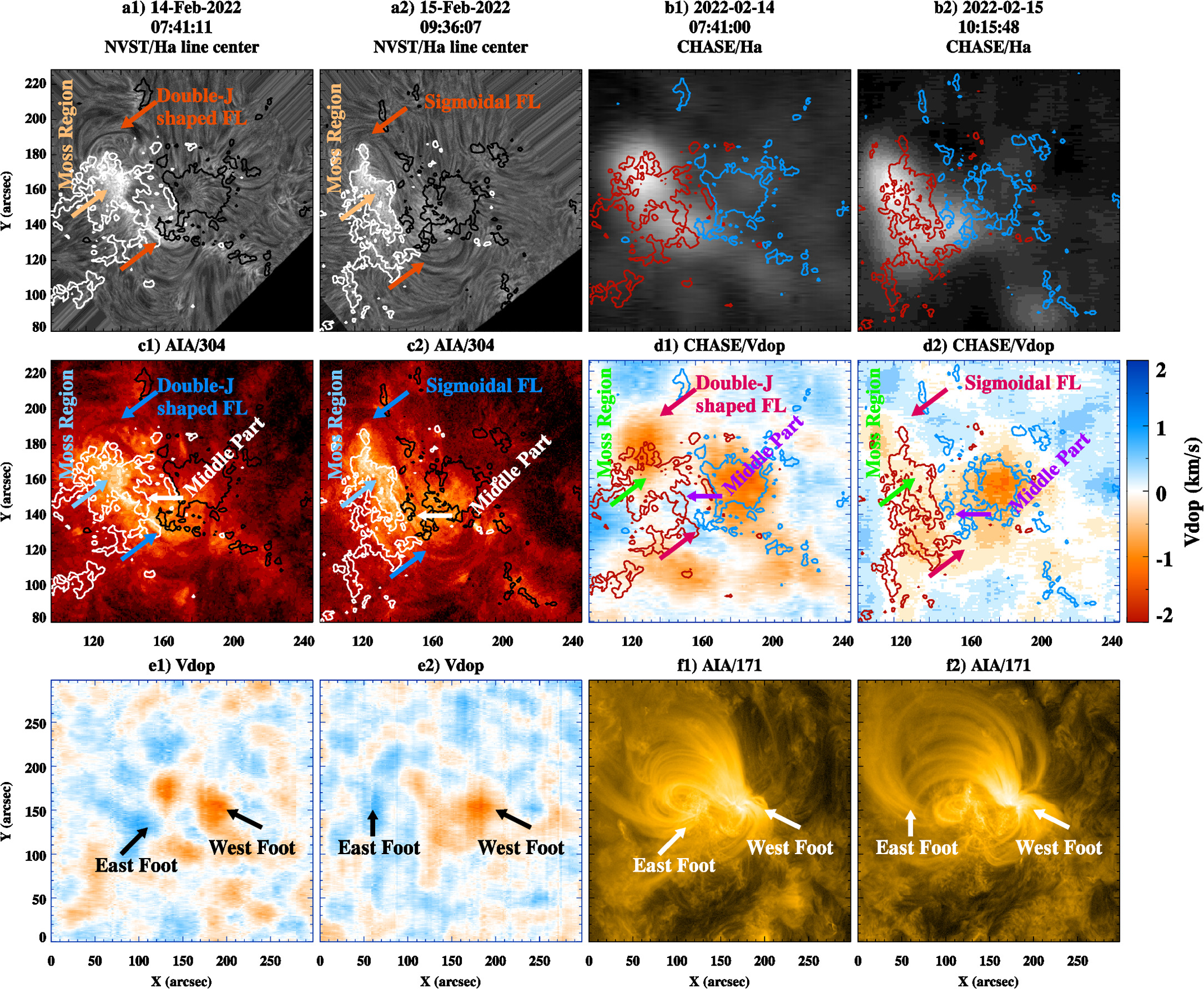
Figure 3. Overview of the observations on February 14 (panels (a1)–(f1)) and 15 (panels (a2)–(f2)). Hα line center images from NVST and CHASE are displayed in panels (a1)–(a2) and (b1)–(b2), respectively. Panels (c1)–(c2) show the images from AIA/304 Å, and Doppler velocities obtained from CHASE are displayed in panels (d1)–(d2). The contours show the LOS magnetic field (Blos) with threshold values of ±100 G. Doppler velocity and AIA/171 Å with a larger FOV are shown in panels (e1)–(e2) and (f1)–(f2), respectively.
Download figure:
Standard image High-resolution imageIn general, there are three distinct regions in AR 12946, i.e., (1) the overlying loops—the cool loops—with the east foot and west foot as identified in the AIA/171 Å images of panels (f1)–(f2) and (2) the brightening-moss regions—footprints of the hot loops—which are well recognized in the Hα and AIA/304 Å observations of panels (a1)–(a2) and (c1)–(c2), as well as (3) the filament that appears as dark structure(s) in panels (a1)–(a2) and (c1)–(c2). Corresponding to the three distinct parts, the Doppler velocity (panels (d1)–(d2)) also shows different features at the chromospheric layer. Although the magnitude of the Doppler velocity at the active region during its relative stable evolution is on the same order of the rest of the parts in the FOV, the magnetic field topology shows different patterns and dominates the different physical behaviors.
The high-resolution observations of NVST show the formation of a sigmoidal filament from two separated J-shaped filaments after around 1 day, and similar evolution was also observed by AIA in 304 Å. As we observe the initial stage of the sigmoidal filament formation, insufficient dark plasma being condensed to the filament channel might be responsible for the relatively faint structure displayed here compared to the eruptive one. Accompanying this transformation, the Doppler velocity exhibits changes, especially around the evolving filament region. At the double-J-shaped stage, the Doppler velocity at the middle part of the separated filaments is dominated by blueshift (panel (d1)), while at the sigmoidal filament stage, a faint LOS velocity of redshift can be identified in the middle part (panel (d2)).
According to the flux cancellation model of flux rope and filament formation (van Ballegooijen & Martens 1989), the flux cancellation on the photosphere is supposed to happen during the sigmoidal filament formation. Such magnetic features at the photosphere are demonstrated in Figure 4. The vector magnetic fields from SHARP/CEA are shown in panels (a1) and (a2). The associated horizontal velocity fields obtained from differential affine velocity estimator for vector magnetograms (DAVE4VMs; Schuck 2008) are displayed in panels (b1) and (b2). The magnetic flux evolution is shown in panel (d). As the location and shape of the active-region PIL where the sigmoidal filament forms change during February 14–15, an adaptive region is selected to ensure a coverage of the similar region around the PIL to calculate the magnetic flux evolution. Such regions at two time steps are shown by the rectangle boxes in white in panels (c1) and (c2).

Figure 4. Panels (a1)–(a2) show the vector magnetic field, with vertical magnetic field (Bver) in the background and the horizontal field (Bhor) overlaid on top as arrows. Red arrows show Bhor at positive polarity, and blue arrows show Bhor at negative polarity. Pink and green contours of ±5 G of the Bver are overlaid. Horizontal flows at the photosphere obtained from DAVE4VM are displayed in panels (b1)–(b2) with purple arrows showing the velocity at positive polarity and green arrows at the negative polarity. Gray and black contours of ±100 G of the Bver are also overlaid. Same vertical magnetic field and the contours of ±5 G of the Bver as in panels (a1) and (a2) are shown in panels (c1) and (c2). Rectangle boxes in white show the regions around PIL where the magnetic flux is calculated. The magnetic flux evolution during February 14–15 is displayed in panel (d); points in pink and green show the positive and negative magnetic flux respectively.
Download figure:
Standard image High-resolution imageAt the photosphere, converging horizontal flows toward the PILs drive the formation of the sigmoidal filament from double-J-shaped arcades as demonstrated in panel (b1)—although note such flow still exists in panel (b2) after the sigmoidal filament has formed. The converging horizontal flow toward the PILs at the photosphere seen in panel (b1) accompanied by the blueshift upflow in the chromosphere in the middle part seen in panel (d1) of Figure 3 are consistent with the picture of ongoing tether-cutting reconnection leading to the formation of a flux rope (e.g., Green & Kliem 2009), which corresponds to the subsequent transition to a sigmoidal filament. Magnetic flux evolution as displayed in panel (d) also shows evidence of cancellation around the PIL, which is a subsequent result of magnetic reconnection. At a later time, the Doppler velocity near the PIL transfers to a faint Doppler redshift downflow in the middle part seen in panel (d2) of Figure 3, which may correspond to the converging flows driven toward the newly formed sigmoidal filament condensations.
There are also moss regions that show intensity enhancement adjacent to the filament during the transition from double-J shape to the sigmoidal shape. The Doppler velocity shows redshift both at the double-J-shaped stage and at the sigmoidal-shape stage for this moss region.
Above the filament and its adjacent moss regions, overlying loops are seen in AIA/171 Å. The overlying loops have a concentrated footprint at the leading sunspot region (west foot as shown in Figure 3 panels (e1)–(e2) and (f1)–(f2)), while the other footprint is spread out in a diffused region around the following sunspot (east foot as shown in Figure 3 panels (e1)–(e2) and (f1)–(f2)). The Doppler velocity at these footprint regions does not differ much between the two time intervals of observations, both showing significant redshift at the west footprint and blueshift at the east one. However, the blueshifted Doppler velocity only appears at the weak magnetic field region of the following sunspot, while the redshifted Doppler velocity dominates at the strong magnetic field region of the leading sunspot. The plasma upflow and downflow that these represent is probably due to a plasma pressure imbalance in the sunspot regions (Rueedi et al. 1992; Solanki et al. 1993), i.e., the so-called "siphon flow."
5.2. Fine Structures inside the Filament
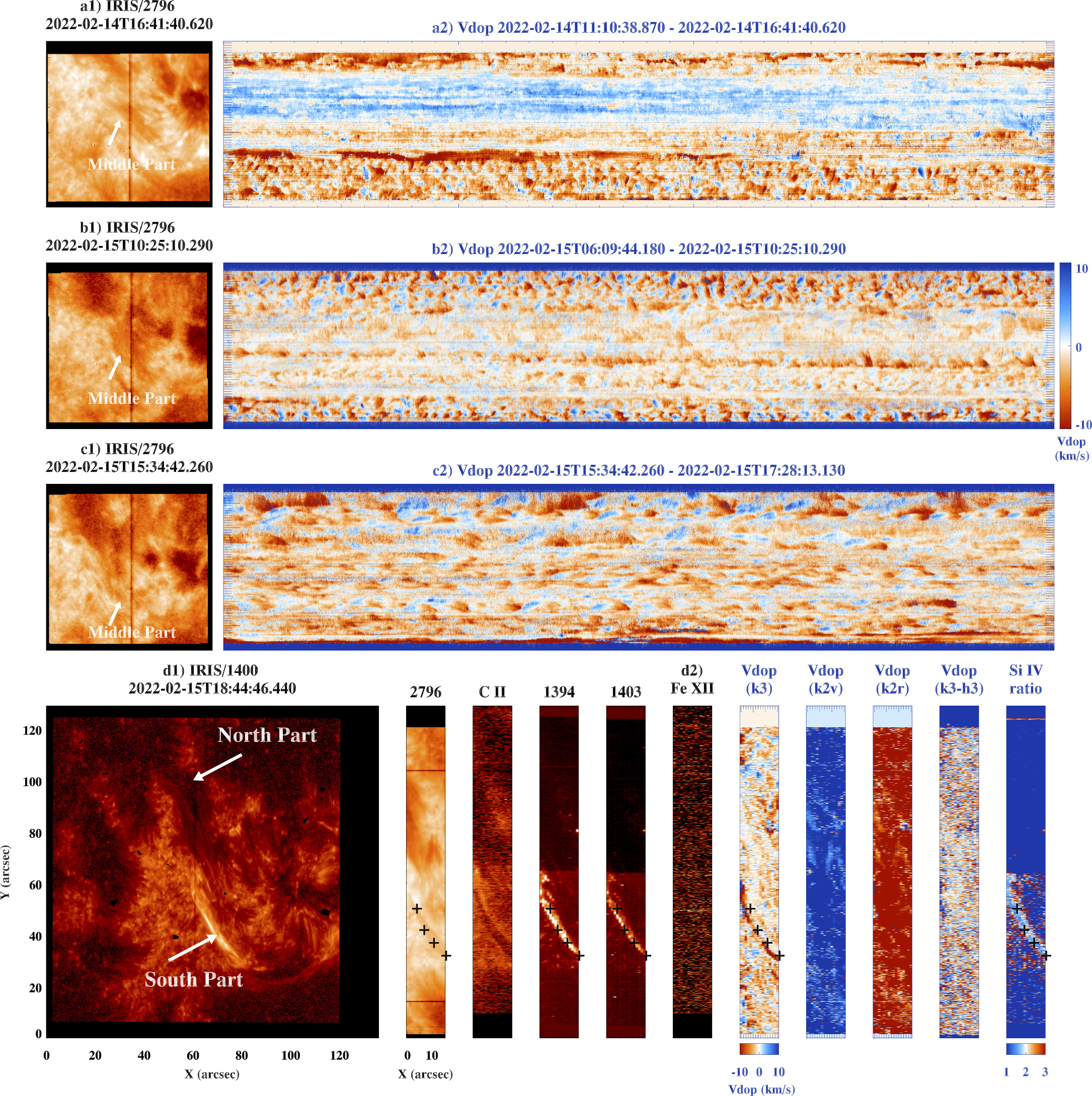
The spectral information in a limited region but with high spatial resolution has been provided by IRIS from February 14 to 15 intermittently. The Doppler velocity at the upper chromosphere is obtained from the Mg ii k line by measuring the displacement of the absorption line center, and velocity at the middle chromosphere is obtained by the line shift of the blue/red peak. The velocity gradient in the upper chromosphere is then obtained through Δvk3–Δvh3, with Δvk3 being the velocity shift obtained for Mg ii k3 line and Δvh3 being the velocity shift obtained for Mg ii h3 line (Pereira et al. 2013). The results are displayed in Figure 5.
Figure 5. Spectroscopic observations from IRIS are displayed at different time ranges. A sit-and-stare model is carried out for the observations in the top three panels. The FOV of the slit-jaw imager (SJI) is displayed for 2796 Å as a vertical red line in the left panels, and the evolution of the obtained Doppler velocity at the location of the slit are displayed in the top right panels, with time on the X-axis. A 16-step raster scanning mode is carried out for the observations as shown in the bottom panels. The FOV of the SJI is shown as a black vertical line in the left panel (d1) in 1400 Å, and the scanning results are displayed in the right panels in (d2). The intensity in the scanning region are displayed in the left five panels from chromosphere to the corona in 2796 Å (∼104.15 K), C ii (∼104.4 K), Si iv 1394/1403 Å (∼104.9 K), and Fe xii (∼106.2 K); the Doppler velocities obtained through the shift of the line center (k3) as well as the blue (k2v) and red peak (k2r) of Mg ii k line are displayed in the following three panels respectively, and the velocity gradient of the upper chromosphere (Δvk3 –Δvh3) is shown next. The Si iv line ratio, which is usually used to indicate the plasma opacity, is shown in the last panel. The intensity enhancement in the south part of the sigmoidal filament is annotated with plus signs in the panels in (d2).
Download figure:
Standard image High-resolution image
Panels (a1)–(c1) show the observations of slit-jaw imager (SJI) in 2796 Å with an FOV of 60'' × 60'' under the sit-and-stare mode; the location of the slit, indicated by the red vertical lines, passes through the middle part of the filament at different stages of its evolution. The obtained Doppler velocity at the locations of the slit for the entire observation time are shown in panels (a2)–(c2). The SJI of 1400 Å at one selected time step under scanning mode is displayed in panel (d1) with FOV of 120'' × 120'', which covers the whole body of the sigmoidal filament. The observation of the 16-step raster scanning is displayed in panel (d2). The intensity images from chromosphere to corona are displayed in the left five columns. The Doppler velocity at different chromospheric layers are shown in the following three columns and the velocity gradient in the middle chromosphere is shown next. The line ratio of Si iv is displayed in the last column, which is usually adopted as a reference for the plasma opacity.
For the sit-and-stare mode carried out at three different time ranges as displayed in panels (a2)–(c2), the Doppler velocity at the upper chromosphere shows significant difference at the middle part of the filament, i.e., upflow dominates around the double-J-shaped stage, while a mixed pattern is found at the sigmoidal-shaped stage. The obtained results are consistent with those derived from CHASE.
In the FOV of the scanning mode, the slit passes through the whole body of the sigmoidal filament. At the displayed time step, the filament fibril at the south part of the sigmoid shows an intensity enhancement at the temperature of the transition region. The ratio of line intensities of Si iv 1394 and 1403 Å is around 2, equal to the ratio of the oscillator strengths of the two lines obtained from CHIANTI (Dere et al. 1997, 2019), which indicates the fibril is optically thin during the brightening (Mathioudakis et al. 1999). The Doppler velocity of the brightening fibril shows apparent redshift but with faint blueshift adjacent. As both of the apparent redshift and the faint blueshift are coming from the fibrils themselves and are well organized along the fibrils, it hints at magnetic braiding during the evolution of the filament (Berger & Asgari-Targhi 2009; Yu et al. 2023).
6. Discussion and Conclusion
By means of the analysis of a filament-embedding active region during its passage across the solar disk, we have obtained the overall characteristics, i.e., the thermal property, the magnetic field, and dynamics at different evolution stages. We find three distinct regions of Doppler velocity at the chromosphere, corresponding to three different structures of the filament-embedding active region. The footprints of the overlying loops—the 1 MK loops that have potential magnetic field—show signatures of "siphon flow" for an extended region, with the upflow appearing at the weak magnetic region, while downflow exists at the strong ones. Such siphon flow, which is induced by pressure difference at the footprints of coronal arcades, has been analyzed theoretically (Noci 1981). Other observations of siphon flow, such as what may drive the movement of the prominence material, has been found before a prominence eruption (Chen et al. 2008). The dynamic features of an emerging flux region obtained from the He i 10830 triplet, which is formed in the upper chromosphere, however, show downflows around 1.5 km s−1 at both footprints of the loops (Xu et al. 2010), which is different from the results here. We attribute this difference to the different evolution stages of the two events. In this work, the active-region magnetic field has already fully emerged, and a stable flow dominates. According to a previous analysis of transition region lines, upflow, which may show the chromosphere evaporation (Tripathi et al. 2012), as well as downflow, which may show the condensation (Del Zanna 2008), have been found respectively in the 1 MK loops. The relationship between the siphon flow found in the Hα line and the other types of velocity found in the transition region or corona needs further investigation and will be crucial for understanding the 3D velocity in the 1 MK loops and the coronal heating problem.
The moss region—footprints of 2–3 MK loops—beneath the overlying 1 MK loops, which has moderately sheared magnetic field lines, shows brightening and apparent downflow. According to observations in the transition region, the moss region is usually found to be downflow dominated (Winebarger et al. 2013) with larger velocity being found at lower temperature although in rare cases, an upflow is also obtained (Dadashi et al. 2012). In the photosphere and chromosphere, represented by the Si i 10827 Å and He i 10830 triplet (Kuckein et al. 2012; Xu et al. 2012), the active-region filament shows upflow, which is flanked by downflow at the faculae region—corresponding to the moss region in this work. Such downflow could probably be associated with the coronal rains that have been simulated with coronal arcades (Fang et al. 2013, 2015; Xia et al. 2017; Li et al. 2022b). With high-resolution observations of He i 10830 Å, ultrafine channels originating from the moss region are suggested to be responsible for the coronal heating in the active region (Ji et al. 2012).
Like in other works (Kuckein et al. 2012; Xu et al. 2012), the middle part of the filament shows distinct kinematic behavior compared to the moss region. In our case, which covers the evolution of the region over a longer time period than other works, we see upflows around the middle part of the filament at the double-J-shaped stage and faint downflows at the sigmoidal-shaped stage. The upflow is around 1–2 km s−1 at the temperature of 103.8 K and around 5 km s−1 at the temperature of 104.15 K. The redshift downflow is, however, around 5 km s−1 at the upper layer and about 1–2 km s−1 at the lower layer.
A filament channel is believed to be necessary for the filament plasma evaporation and condensation, yet observations capturing both the formation of the filament channel and then the condensation are rare. Based on magnetic flux evolution at the photosphere (Yang et al. 2021) or EUV loop emission (Li et al. 2021), magnetic reconnection has been suggested as a mechanism for filament-channel formation. In this work, the magnetic reconnection that produces the filament-channel formation is confirmed not only through the converging flow at the photosphere but also by the dynamic features of a reconnection outflow/upflow at two different layers of the chromosphere. The filament-channel formation is followed by the filament condensation downflow in the same place, which is reported for the first time here.
Plasma condensation toward magnetic dips has been observed in the coronal line as dark fibril material that appears to have evaporated near the footprint of a filament channel (Li et al. 2021; Yang et al. 2021). Our analysis includes chromospheric observations of the Hα and IRIS Mg ii lines, which demonstrates direct evidence of the dynamics in the low chromosphere, including possible magnetic dip formation and the probable falling of cold and condensed filament plasma into the low-lying dips after the hot plasma condensation. In the future, such observations may be further augmented with high-resolution observations of CHASE, which have been available since 2022 August 4.
The main body of the filament, which has sheared magnetic field lines along the PIL, is observed with spectral lines with high resolution at a later time. We investigate the kinematic and thermal dynamic evolution for filament fibril brightenings specifically. The brightenings of fibrils are accompanied by the upflow and downflow of adjacent regions, indicating the braiding of fine structures inside the large-scale filament. The observations also show a transition from optically thick to optically thin during the brightenings.
In this work, we have been limited to the FOV of IRIS so that the overall kinematic features of the moss region in the upper chromosphere and transition region are missing. We have carried out a larger-raster FOV in a more recent observation, which we expect will provide more constraints on these different layers. Finally, we look forward to the future EUV High-Throughput Spectroscopic Telescope (Shimizu et al. 2020) and the Multi-slit Solar Explorer (De Pontieu et al. 2020; Cheung et al. 2022), which together will provide abundant plasma information from chromosphere to the corona with subarcsecond resolution and high temporal cadence in the FOV of AR scale, which enables a comprehensive understanding of the possible heating mechanisms at different parts of the active region as well as the mass loading of the embedded filament.
Acknowledgments
We thank the referee for constructive suggestions to greatly improve the manuscript. We thank Dr. Ye Qiu for verifying the Doppler velocity obtained in this work. The data used in this paper were obtained with the New Vacuum Solar Telescope in Fuxian Solar Observatory of Yunnan Astronomical Observatory, CAS. CHASE mission is supported by China National Space Administration. IRIS is a NASA small explorer mission developed and operated by LMSAL with mission operations executed at NASA Ames Research Center and major contributions to downlink communications funded by ESA and the Norwegian Space Centre. Courtesy of NASA/SDO and the AIA, EVE, and HMI science teams. J.Z. acknowledges the support by the National Key R&D Program of China (grant No. 2022YFF0503001), the Strategic Priority Research Program of the Chinese Academy of Sciences (grant No. XDB0560302), and the Youth Innovation Promotion Association CAS (grant No. 2023333). This work is also supported by the National Natural Science Foundations of China (grant Nos. 12233012, 11973012, 12333009, and 11820101002). The National Center for Atmospheric Research is a major facility sponsored by the NSF under Cooperative Agreement No. 1852977.