
Abstract
Backscatter coefficient analysis methods for biological tissues have been clinically applied but assume a homogeneous scattering medium. In addition, there are few examples of actual measurement studies in the HF band, and the consistency with theory has not been sufficiently confirmed. In this paper, the effect of correlations among scatterer positions on backscattering was investigated by performing experiments on inhomogeneous media having two types of scattering source with different structural and acoustic properties. In the echo data of phantoms containing two types of scatterer acquired by multiple sensors, the power and frequency dependence of the backscatter coefficient were different from theoretical calculations due to the interference effects of each scatterer. The effect of interference between the two types of scatterer was confirmed to be particularly strong for echoes acquired by the sensor at high intensity and HF, or for a higher number density of strong scatterers.
Export citation and abstract BibTeX RIS
1. Introduction
Quantitative ultrasound (QUS) is useful for the noninvasive evaluation of diseases of various biological tissues, such as the liver, breast, lymph nodes, skin, and bone. In particular, amplitude envelope statistics, 1–6) attenuation coefficients, 7–9) backscatter coefficients (BSCs), 10–14) and elastography 15–20) have attracted attention in clinical practice, and tools for evaluating QUS parameters that were developed using these techniques have been implemented in clinical ultrasound systems.
As the BSC depends on physical quantities such as the scatterer diameter, volume fraction, and relative acoustic impedance difference between the scatterers and surrounding medium, these physical quantities can be estimated by comparing the measured BSC with the BSC predicted using a theoretical model. 21,22) It has been reported that the evaluation of fatty liver, 23,24) dermal lymphedema, 25–27) thyroid tumors, 28,29) and trabecular bone 30) is possible using the BSC as an indicator. Basic BSC evaluations have been widely conducted using single-element concave transducers.
There have also been reports of evaluations adopting multiple frequency bands, 31,32) plane-wave compound imaging, 33–35) and spatial synthesis 10,12) to improve evaluation accuracy. Omura et al. used multiple ultrasound scanners to acquire signals adopting two beamforming methods, namely line-by-line beamforming with focused imaging and parallel beamforming with plane-wave imaging, and verified the variation in the BSC. 35) They confirmed that the BSC could be evaluated with equal accuracy using the two signal acquisition methods, indicating the possibility of BSC analysis through parallel beamforming with plane-wave imaging.
Besides adopting beamforming methods to evaluate the BSC, another challenge is to evaluate the quantitative ultrasonic parameters (e.g. the effective diameter and volume fraction of scatterers) in the presence of various types of scattering source mixed in biological tissues. Thus, it is of particular interest to examine the effects and interference of various populations of scatterers in a tissue. Scattering sources in a biological tissue are densely intermingled, with there being multiple sources within the point spread function (PSF) of the transducer. The backscatter characterization is usually based on the spectral analysis of the speckle signal, which is generated by interference between individual scatterers. It is therefore necessary to understand the effects of wave interference generated by correlations among scatterer positions. The effect of spatial correlation in a homogeneously distributed medium with one type of scatterer is well understood. Franceschini et al. investigated a scattering model from the perspective of explaining experimental BSCs of cell-pellet biophantoms with a single structural and acoustic parameter set. 36) They reported that the scattering model provided satisfactory estimates of the impedance and size of the scatterers. However, little attention has been paid to the spatial correlations between scatterers in heterogeneous media containing a mixture of scatterers with different acoustic properties. In addition, there are few examples of actual measurement studies in the HF band, and the consistency with theory has not been sufficiently confirmed. Therefore, the interpretation of BSCs of complex biological tissues first requires an understanding of ultrasonic backscattering from a biological phantom with known scattering conditions and intermixed scattering structures.
In this study, we examined the effect of interference between scatterers and compared the BSCs of phantoms having different volume ratios of two types of scatterer. Using a laboratory-made ultrasonic scanner and two types of single concave transducer, we evaluated the BSCs at low and high frequencies. We also evaluated the BSCs using a research platform scanner and a very-HF linear array probe. Specifically, signals were acquired adopting the parallel beamforming method with plane-wave imaging and BSC analysis was performed.
2. Materials and methods
2.1. Tissue-mimicking phantoms of multiple types of scatterer
Seven different rectangular phantoms (8 cm in width × 2 cm in length × 4 cm in height) were prepared as reference and evaluated phantoms. The solvents of each phantom were 2 wt% agar (A1296; Sigma-Aldrich, MO, USA) and distilled water. The weak scatterers were nylon spheres with an average particle diameter of 5 μm (ORGASOL 2001 EXD NAT 1; Arkema, Colombes, France) and the strong scatterers were acrylic spheres with an average particle diameter of 20 μm (MX-2000; Soken, Aichi, Japan). The intrinsic acoustic impedances were 1.493 and 1.665 MRayl, respectively. These scatterers were mixed at various volume fractions as given in Table I.
Table I. Phantom composition and acoustic properties.
| Phantom | A | B | C | D | E | F | G |
|---|---|---|---|---|---|---|---|
| Volume fraction of scatter 1 [%] | 0.5 | — | 0.5 | 0.5 | 0.5 | 2 | 5 |
| Volume fraction of scatter 2 [%] | — | 0.3 | 0.1 | 0.3 | 0.5 | 0.3 | 0.3 |
Scatterer 1: nylon with diameter of 5 μm, scatterer 2: acrylic with diameter of 20 μm.
Phantoms A and B were homogeneous media with only one type of scatterer. They were created as a reference medium for which the spatial correlations between scatterers were known for comparison with phantoms containing the two types of scatterer. These phantoms had volume fractions sufficiently small for the scatterers to be far enough apart so as not to interfere with each other. Phantom A was created so that the scattering intensity was equivalent to that of a normal liver. Phantom B represented the case that only fat droplets were present, which is not possible in actual living tissue. Phantoms C, D, and E represented the case of different fractions of fat droplets (strong scatterers) mixed within the normal liver (weak scatterers) whereas phantoms D, F, and G represented the case of a constant fraction of fat droplets and different fractions of liver components. By comparing the BSCs of these phantoms, the fractions (distribution) of the two types of scatterer and the effects of scattering and mutual interference between the two scatterer populations were evaluated. In particular, this paper assumes that there is interference due to the superposition of scattered signals.
2.2. Data acquisition using a laboratory-made scanner
Three-dimensional RF echo signals were acquired using a laboratory-made ultrasonic scanner and two types of single-element concave transducer [transducer I (V327; Olympus, Tokyo, Japan) and transducer II (PT35; TORAY, Tokyo, Japan)]. The center frequency and −6 dB wide frequency band of transducer I were 10 MHz and 7–13 MHz whereas those of transducer II were 30 MHz and 20–37 MHz. The depths of focus were 19.7 and 10 mm and the f-numbers were 2.10 and 1.85 for transducers I and II, respectively. For echo data acquisition, pulser receiver I (model 5800; Olympus, Tokyo, Japan) for the V327 transducer and pulser receiver II (DPR500; JSR Ultrasonics, NY, USA) for the PT35 transducer were used to excite negative impulses to the element for transmission. The received echo signals were band-pass filtered at 1–35 MHz and 30–300 MHz, respectively, by the receiver circuit in each pulser receiver. Each echo signal was digitized at 12 bits using an oscilloscope (HDO6104; Teledyne LeCroy, NY, USA) set at a sampling frequency of 250 MHz. The parameters of the PSF near the focus of each transducer are given in Table II. The PSFs in the lateral and axial directions at each depth were calculated at −6 dB of the normalized envelope amplitude for a pin target placed in degassed water at 21.7 °C. The transducer was fixed to a triaxial linear rail (MTN100CC, Newport) and mechanically scanned in the lateral and elevation directions. The phantom was fixed in degassed water at 22 °C–24 °C. Echo signals were acquired by insonifying the phantom from the top surface. The depth of field was 17.8–21.5 mm for the V327 transducer and 9.7–10.7 mm for the PT35 transducer, and the phantom surfaces were thus set at 17 and 9 mm, respectively, to cover the area of analysis within the depth of field. The scan pitch was 30 μm in both the lateral and axial directions. Three-dimensional RF echo signals of 4096 pixels in the depth direction × 501 pixels in the lateral direction × 101 pixels in the axial direction were acquired for all phantoms. The data acquisition and motor stage control were conducted using LabVIEW (National Instruments, TX, USA).
Table II. PSF near focus for each sensor.
| Axial [μm] | Lateral [μm] | |
|---|---|---|
| V327 | 109 | 300 |
| PT35 | 42 | 95 |
| L39-21gD | 80 | 120 |
2.3. Data acquisition using the research-platform scanner
Two-dimensional RF echo signals were acquired using a research-platform scanner (Vantage256; Verasonics, WA, USA) and a linear array probe (L39–21gD; Daxsonics Ultrasound Inc., Halifax, Canada ). The center frequency and −6 dB bandwidth were 31.25 MHz and 20–36 MHz, respectively. The element pitch and number of elements were 0.055 mm and 128 channels, respectively. The lens focus of the probe was approximately 6.5 mm. Each echo signal was digitized at 14 bits with the sampling frequency set at 4/3 times the center frequency. In addition, the acquired data were up-sampled by a factor of 3 in the depth direction to produce data with a sampling frequency that was effectively 4 times the center frequency. In this case, the Nyquist frequency was 20.833 MHz, and the signal to be evaluated was folded back to the band below the Nyquist frequency. As the spectrum could be evaluated even if it was folded back as long as it did not appear in the band of other energy pixels, a 20–36 MHz band-pass filter was applied to remove the low-frequency signal added to the signal to be evaluated after aliasing. This made it possible to evaluate signals in the region of frequencies higher than the Nyquist frequency. 37) The PSF at the point of highest resolution is given in Table II. RF data of each B-mode plane of each phantom were acquired by plane wave imaging with parallel beamforming. Plane waves were steered at 11 angles (0°, ±1°, ±2°, ±3°, ±4°, and ±5°), and the analysis signal was generated by combining the plane waves through a delay and sum operation.
2.4. Calculation of the speed of sound and attenuation coefficient
The speed of sound and attenuation coefficient were evaluated for each phantom adopting the reflection method before BSC analysis. Three-dimensional RF echo signals were acquired using single-element plane transducer III (V312; Olympus, Tokyo, Japan) in the same setting as for transducer I in Sect. 2.2. The center frequency and −6 dB wide frequency band of transducer Ⅲ were 10 MHz and 7–13 MHz. In addition, echo signals were acquired using transducer II under similar conditions. An acrylic plate was placed on top of the sound absorber, and the echo signals were acquired with and without the sample while maintaining the positional relationship between the transducer and acrylic plate. 38) The transducer was set at the depth at which the signal from the acrylic plate was a maximum. The speed of sound was calculated from the time of flight (TOF) based on the time difference between the maximum amplitude returned from the sample and the acrylic plate:

where  is the TOF from the sample surface,
  is the TOF from the back,
  is the TOF from the acrylic plate after the sample passed through, and
  is the TOF from the acrylic plate at the same position as in the measurement.
  is the speed of sound in water. The thickness d of the sample was calculated as
  The attenuation rate of the phantom,
  [dB/cm], was calculated using the power spectra with and without the sample:

where  is the frequency in MHz,
  is the power spectrum through the phantom, and
  is the power spectrum without the sample. The attenuation rate can be considered to be the same as the absorption rate when the frequency is somewhat low, when the absorption attenuation is dominant, or when scattering is negligible in a relatively homogeneous medium. In particular, in the frequency bandwidth of 1–10 MHz used for a clinical ultrasonic imaging system, the attenuation rate can often be approximated as being proportional to the first power of the frequency. Therefore, the attenuation coefficient
  [dB/cm/MHz] is written as
  Meanwhile, the frequency dependence of attenuation is considered to be an important characteristic in the frequency bandwidth above 10 MHz, and the dependence of attenuation on frequency is described as
  where
where  is the attenuation coefficient in units of dB/cm/MHzn
and
is the attenuation coefficient in units of dB/cm/MHzn
and  is the exponent to be determined.
39) Therefore, the parameters were approximated by the equations
is the exponent to be determined.
39) Therefore, the parameters were approximated by the equations  and
and  for the signals measured with transducers III and II, respectively, adopting the least-squares method with a bandwidth of −6 dB.
The speed of sound of all phantoms calculated using the different transducers are given in Table III, and the attenuation coefficients are given in Table IV.
Table III. Result of speed of sound estimation [m/s].
| A | B | C | D | E | F | G | |
|---|---|---|---|---|---|---|---|
| Transducer Ⅲ | 1494.4 | 1501.6 | 1490.1 | 1491.3 | 1489.8 | 1499.8 | 1520.5 |
| Transducer Ⅱ | 1491.6 | 1485.7 | 1489.4 | 1484.0 | 1484.1 | 1496.4 | 1507.1 |
Table IV. Frequency dependence of attenuation [dB/cm].
| A | B | C | D | E | F | G | |
|---|---|---|---|---|---|---|---|
| Transducer Ⅲ | 0.11f | 0.13f | 0.22f | 0.23f | 0.27f | 0.29f | 0.46f |
| Transducer Ⅱ | 1.3 × 10⁻⁵ f3.5 | 1.1 × 10⁻⁷ f5.3 | 8.9 × 10⁻⁸ f5.1 | 1.3 × 10⁻⁶ f4.6 | 1.7 × 10⁻⁴ f3.3 | 3.8 × 10⁻⁵ f3.7 | 0.05f1.8 |
2.5. Backscatter coefficient analysis using the reference phantom method
The BSC was calculated using the reference phantom method. 40) The reference phantom method assumes that the attenuation properties and BSC of the reference phantom, as well as the attenuation properties of the phantom to be characterized, are known a priori. Using a phantom with known scattering conditions as reference echo data, the BSC can be evaluated robustly by correcting the sound field of the transmitting and receiving systems when evaluating a medium with complex beam diffraction effects, such as a linear array probe, or a medium with complex scatterer structures, such as biological tissue. Array probes can be used to evaluate the BSC with high robustness and are thus widely used. In this study, regions of interest (ROIs) were set up to analyze local RF signal characteristics, and the BSC for each ROI was estimated. The ROIs were scanned within the depth of field of each transducer. The ROI size was 10 times the wavelength at the center frequency of the transducer in the depth direction and 10 uncorrelated echo lines in the lateral direction. Under these conditions, Transducers I and II and the linear array probe were correlated with eight, three, and five adjacent signals, respectively, such that the ROI sizes in the lateral direction were 80, 30, and 50 lines, respectively. The measured BSC was estimated as
where  is the average of the power spectra of the RF signals from the phantom to be characterized and
  is the power spectrum of the reference medium. The frequency response of the measured echo signal includes a component of attenuation that occurs during ultrasonic wave propagation. Therefore, the last exponential term in Eq. (3) corrects for the attenuation effects in the analyzed ROI.
  and
and  are attenuation coefficients,
  is the distance from the scattering medium surface to the start of the analysis window, and
  is the size of the analysis window.
41)
is the size of the analysis window.
41)
The theoretical value of  for phantom A was used as the reference phantom. In this study, the reference phantom was taken as Phantom A. The theoretical value was calculated as
36)
for phantom A was used as the reference phantom. In this study, the reference phantom was taken as Phantom A. The theoretical value was calculated as
36)

where  is the number density of scatterers and
  is the radial probability density function (PDF) of scatterers. To compute the radial PDF, the scatterer areas were calculated through optical microscopy (before the scatterers were embedded in the agar phantom). The particle radii were calculated from the scatterer areas by assuming that the scatterers had circular cross-sections. This was done for approximately 40 000 scatterers. From the mean and variance of the scatterer radii, the PDF was calculated on the basis of a normal kernel function. The specific cross section of a single elastic sphere
  was computed adopting theory developed by Faran.
42) This theory provides an exact solution for the scattering of sound by a solid sphere in a surrounding fluid medium and therefore includes transversal waves in addition to compressional waves. The structure factor
was computed adopting theory developed by Faran.
42) This theory provides an exact solution for the scattering of sound by a solid sphere in a surrounding fluid medium and therefore includes transversal waves in addition to compressional waves. The structure factor  allows the modeling of the interference effects generated by correlation among scatterer positions, particularly when the randomness of the scatterer's position is impaired. r, k, and
  are the particle size, wavenumber, and volume fraction of the scatterer, respectively. The Faran model commonly used in BSC evaluation at this higher order assumes that the surrounding medium is water, whereas the target of evaluation in this study is agar, and there is a difference in assumption. Given that these assumptions are different, it is significant to compare the differences as BSC values. In addition, this model considers only the interference effects due to correlations between the positions of one type of scatterer.
To verify the effects of interference between two types of scatterer, the deviation between the evaluated BSC and the theoretical value of the BSC was calculated. The theoretical value of the BSC was calculated in the same way as for equation(4). The average deviation is defined as
where  is the frequency band used in the analysis. Deviation [dB] evaluates the difference between the logarithmic values of the respective BSCs.
3. Results
3.1. BSC evaluation of phantoms with one type of scatterer
To understand the characteristics of the phantoms used for reference, phantoms A and B containing only one type of scatterer were measured with the two single-element concave transducers and a linear probe. B-mode images of phantoms A and B acquired using transducer I, transducer II, and the linear array probe are shown in Fig. 1. Each B-mode image was normalized by the maximum amplitude value for phantom B represents an arbitrary single frame. As the size and acoustic impedance of scatterers type 2 were higher than those of scatterers type 1, the echo amplitude was largest for phantom B.

Fig. 1. B-mode images of (a-1)–(c-1) phantom A and (a-2)–(c-2) phantom B acquired with (a) transducer I, (b) transducer II, and (c) the linear array probe.
Download figure:
Standard image High-resolution imageIn phantom A, there were 749, 28.9, and 88 scatterers according to the PSFs of transducer I, transducer II, and the linear array probe, respectively; these numbers corresponded to speckling [Figs. 1(a-1)–1(c-1)]. In phantom B, there were 7.02, 0.27, and 0.82 scatterers in the PSFs of transducer I, transducer II, and the linear array probe, respectively. The scatterers imaged with transducer I thus had a speckle pattern. Transducer II can be considered a point scattering source. However, there were more scatterers in the PSF of the linear array probe than in the PSF of the transducer II,, and some areas were thus seen as speckles [Figs. 1(a-2)–1(c-2)].
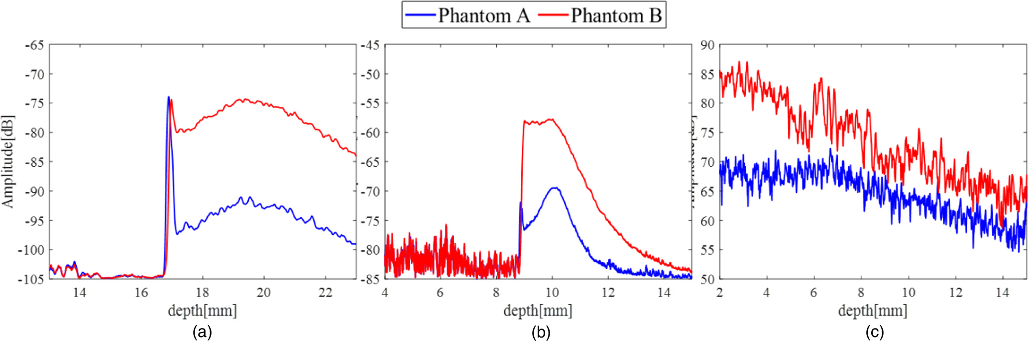
Fig. 2. Amplitude envelopes of phantoms A and B acquired with (a)transducer I, (b) transducer II, and (c) the linear array probe.
Download figure:
Standard image High-resolution imageThe amplitude envelopes of phantoms A and B acquired by each sensor are shown in Fig. 2. This is the result averaged over the lateral and elevation directions. The f-numbers of transducers I and II were 2.10 and 1.85, respectively, and the sound pressure gradient was steep for transducer II. Therefore, the signal below 12 mm was equivalent to the amplitude in the water region, and the signal-to-noise ratio was not sufficiently high [Fig. 2(b)]. Meanwhile, the data recorded with the linear array probe had high signal strength even at depth [Fig. 2(c)].
The frequency spectra of phantoms A and B acquired by each sensor are shown in Fig. 3. The frequency spectrum was calculated by cutting the signal of 10 wavelengths centered on the focus of each sensor in the depth direction. Each frequency spectrum was normalized by the maximum value for each phantom. Transducer I had a narrow effective bandwidth [Fig. 3(a)] whereas transducer II and the linear array probe had a wide effective frequency band in the very HF range [Figs. 3(b), 3(c)]. Meanwhile, a comparison of the amplitude envelopes and frequency spectra of transducer II and the linear array probe shows that the linear array probe had large variation in values and a low signal-to-noise ratio. The linear array probe used in this study had an element pitch longer than the wavelength, which creates grating lobes. In other words, the grating lobe artifact in the signal caused a large value variation.
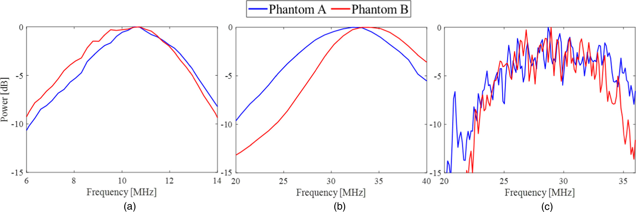
Fig. 3. Power spectrums of phantoms A and B acquired with (a) transducer I, (b) transducer II, and (c) the linear array probe.
Download figure:
Standard image High-resolution imageThe BSC measurements made for phantoms A and B using each sensor and their respective theoretical values are shown in Fig. 4. Phantom A was self-referencing, and the sound field and attenuation corrections could thus be performed with high accuracy, and the results were in agreement with theoretical values. For phantom B, the results for transducer I agreed with the theoretical values, confirming the high precision of the evaluation [Fig. 4(a)]. However, in the HF bandwidth (>20 MHz), the BSC measurement of phantom B did not match the theoretically predicted BSC frequency dependence, and the deviation was large [Figs. 4(b), 4(c)]. The agreement between the Faran model and the measured BSC in the HF band was unsatisfactory, with the theoretical prediction of the BSC having a dip near 23 MHz and a sharp peak around 27 MHz, whereas the measured BSC followed a smooth curve. As a preliminary study, a similar study was conducted on several phantoms with different volume fractions containing only strong scatterers with diameters of 20 μm, but no characteristic frequency response identified in the theoretical values was observed, regardless of the scatterer density. This is assumed to be because the Faran model using theoretical calculations requires the spherical scatterer to exist in water, whereas the actual phantom exists in an agar medium. Water and agar gels have different viscoelasticity, and agar particles too small to be visually recognized may be present around the spherical scatterer, creating a locally structured scattering source. In fact, even in the lower frequency bands, the measured BSC evaluation results often do not match the theoretical values calculated by the Faran model, so it is assumed that this is more pronounced in the higher frequency bands. 31)
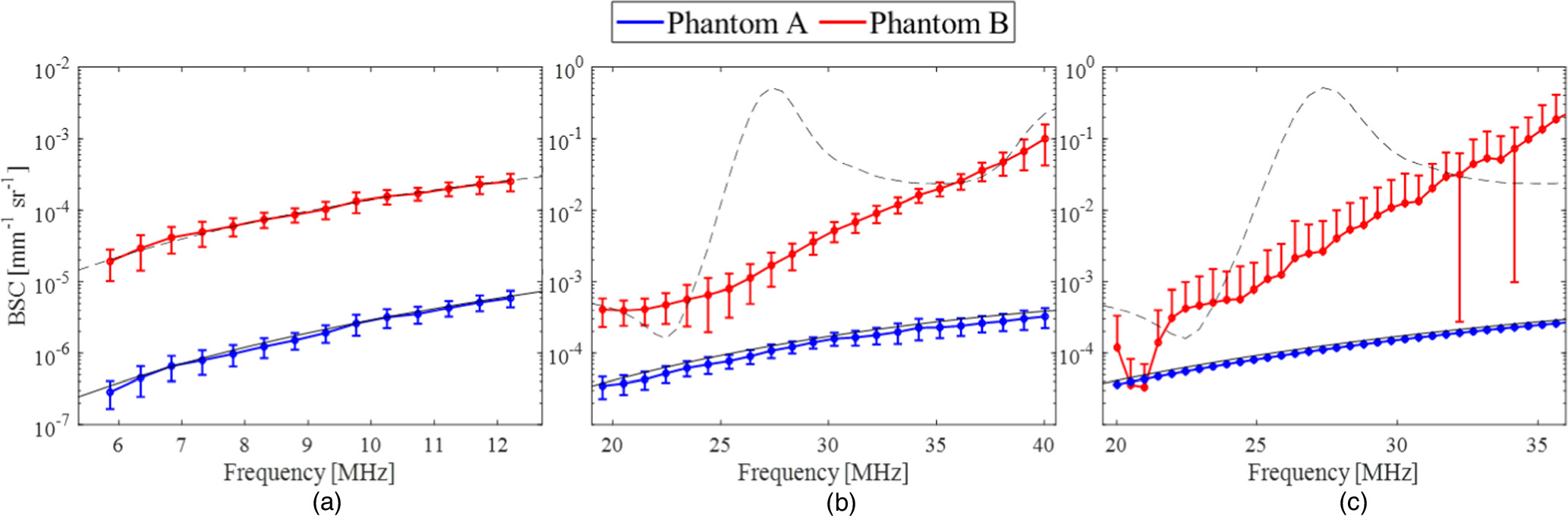
Fig. 4. Backscatter coefficients of phantoms A and B acquired with (a)transducer I, (b) transducer II, and (c) the linear array probe and theoretical values.
Download figure:
Standard image High-resolution image3.2. BSC evaluation of phantoms with two types of scatterer
3.2.1. Effects of increasing the number of strong scatterers
The BSC measurements of phantoms with only one type of scatterer mixed in confirmed the effect of the number density of strong scatterers on the backscattering characteristics. B-mode images of phantoms C, D, and E acquired using transducer I, transducer II, and the linear array probe are shown in Fig. 5. The method of normalizing the B-mode images was the same as that adopted for Figs. 1(a-2)–1(c-2). A comparison of the results for phantoms C, D, and E obtained using transducer I revealed that the echo amplitude increased with the scatterer number density [Fig. 5(a)]. In the case that transducer II was used, the amplitude did not change as the number density increased [Fig. 5(b)]. Meanwhile, in the case that the linear array probe was used, the amplitude decreased as the number density increased. In particular, strong scatterers were identifiable as point scattering sources, with the amplitude progressively decreasing as the number of strong scatterers increased [Fig. 5(c)].

Fig. 5. B-mode images of (a-1)–(c-1) phantom C, (a-2)–(c-2) phantom D,and (a-3)–(c-3) phantom E acquired with (a) transducer I, (b) transducer II, and (c) the linear array probe.
Download figure:
Standard image High-resolution imageThe amplitude envelopes of phantoms A, B, C, D, and E for each sensor are shown in Fig. 6. The figure also presents results for phantoms A and B for comparison. The signal intensity from the water–phantom interface was similar for all phantoms [Figs. 6(a), 6(b)]. This can be explained in that the number density of scatterers in phantoms A, B, C, D, and E is sufficiently low (<1%) for the speed of sound and acoustic impedance to be similar across phantoms A, B, C, D, and E and the amplitudes of the specular echo from the water–phantom interfaces to also be similar. The amplitudes acquired by the linear array probe showed that the scatterer number density increased in the order of phantoms B, D, and E but the amplitude decreased in the order of phantoms B, D, and E [Fig. 6(c)].

Fig. 6. Amplitude envelopes of phantoms A, B, C, D, and E acquired with (a) transducer I, (b) transducer II, and (c) the linear array probe.
Download figure:
Standard image High-resolution imageThe frequency spectra of phantoms A, B, C, D, and E recorded with transducer I, II, and the linear array probe are shown in Fig. 7. The power was normalized by the maximum value of each phantom. For transducer I, the frequency bands (bandwidths) of phantoms C, D, and E at −6 dB were 7.4–13.3 MHz (5.9 MHz), 7.0–13.1 MHz (6.1 MHz), and 6.8–13.0 MHz (6.2 MHz), respectively [Fig. 7(a)]. For transducer II and the linear array probe, the signal was stronger at low frequency owing to the higher number density of scatterers in the PSF for phantoms C, D, and E and weaker at HF owing to the higher scattering attenuation [Figs. 7(b), 7(c)].
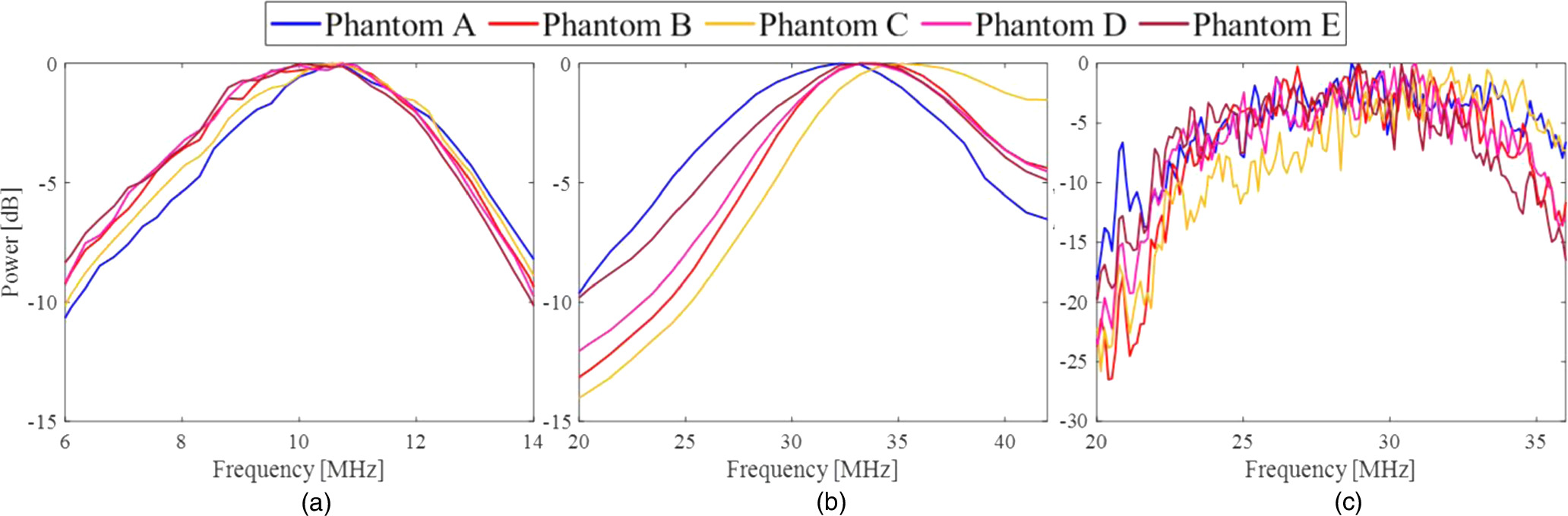
Fig. 7. Power spectrums of phantoms A, B, C, D, and E acquired with (a) transducer I, (b) transducer II, and (c) the linear array probe.
Download figure:
Standard image High-resolution imageThe BSCs for phantoms C, D, and E measured with each transducer are shown in Fig. 8. The figure also shows the theoretical predictions of the BSCs. The theoretical value for the two-scatterer mixed phantom was obtained by substituting the PDF of the particle size for each phantom into the PDF in Eq. (4). In the other words, the scattering of the polydisperse medium was calculated as the sum of the scattering from several monodisperse subsystems weighted by the radial PDF. Interference effects generated by the spatial correlations between scatterers were taken into account through the structure factor, by assuming that the scatterer of a certain size was surrounded by scatterers of the same size. However, the mutual interaction between the two types of scatterer was not considered. There was no difference in the frequency dependence of each phantom for transducer I. As the number of strong scatterers increased, the magnitude of the measured BSC was higher, and the BSCs measured for phantoms C were consistent with the theoretical values [Fig. 8(a)]. For transducer II, the measured BSCs for the phantom with two mixed scatterers were similar to the measured BSCs for phantom B and largely different from the theoretical values. In particular, the properties of phantom D were strongly consistent with those of phantom B [Fig. 8(b)]. The BSCs measured with the linear array probe were lower than those of phantom B, and the deviation from the theoretical value was large. A comparison across phantoms C, D, and E reveals that the BSC decreased as the scatterer number density increased, especially in the frequency range of 32–38 MHz [Fig. 8(c)].
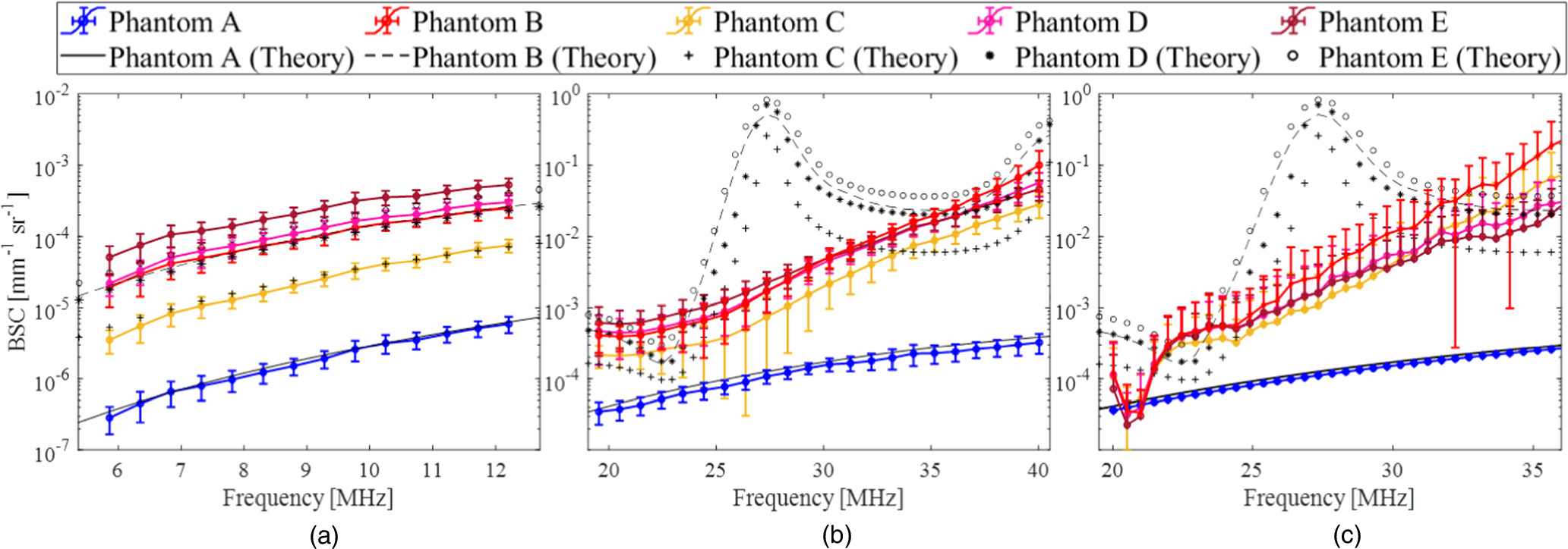
Fig. 8. Backscatter coefficients of phantoms A, B, C, D, and E acquired using (a) transducer I, (b) transducer II, and (c) the linear array probe and theoretical values.
Download figure:
Standard image High-resolution imageThe deviations between the measured and theoretical BSCs are shown in Fig. 9. Although there is a large difference between the measured and theoretical values under the conditions of this study, the deviation was calculated to compare and quantify the differences in properties between phantoms on the basis of differences in physical conditions from theory. Phantom B had only one type of scatterer, but the deviation of its measured BSC from the theoretical value was so large that it was difficult to compare with the deviation calculated using Eq. (5) [Fig. 4(b)]. Therefore, the deviations between the measured and theoretical BSCs of the other phantoms were normalized at each frequency such that the deviation for phantom B was zero, and the mean and standard deviation of the deviation between the measured and theoretical BSCs were calculated. In the preliminary study described in Sect. 3.1, the average BSC in phantoms with different volume fractions containing only strong scatterers with a diameter of 20 μm decreased as in Fig. 4, however, no increase in deviation with increasing volume fraction was observed. In other words, the main reason for the larger deviation with increasing volume fraction in Fig. 4 is thought to be the presence of two types of scatterers. The theoretical value of the BSC was obtained using a model that did not take into account the interference between the two types of scatterer, whereas the measurements included the interference and the deviation thus indicates the degree of such interference. A smaller standard deviation indicates a smaller frequency-dependent deviation. As the evaluation of phantom A was self-referencing and the evaluation was highly accurate in all modalities, the deviation was not calculated for phantom A. The mean and standard deviation of the deviation for transducer I were within 3 dB, indicating a high degree of agreement with the theoretical values. The mean deviation for transducer II and the linear array probe decreased with increasing scatterer number density, with the standard deviation of the deviation being larger for the linear array probe.
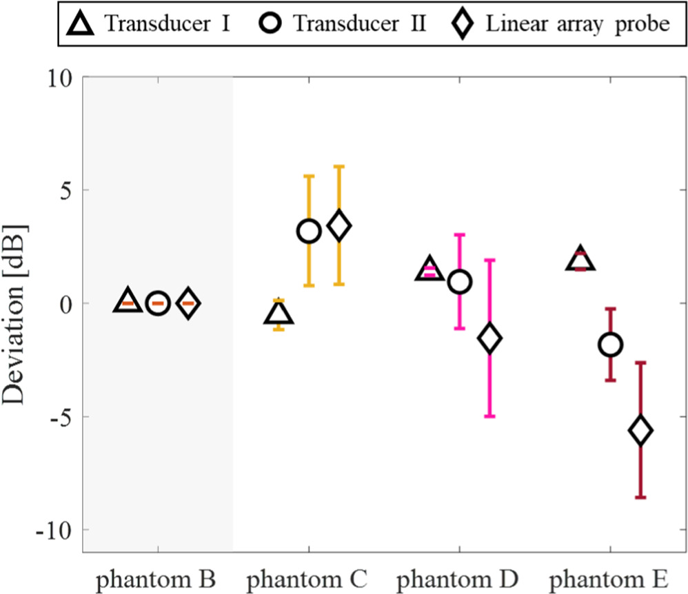
Fig. 9. Deviations between the estimated backscatter coefficients for phantoms B, C, D, and E and the theoretical values calculated using the mathematical model.
Download figure:
Standard image High-resolution image3.2.2. Effects of increasing the number of weak scatterers
Previous studies considered only the case of increasing the number of strong scatterers, but this is insufficient to verify the effects of interference. 43) To confirm the effect of increasing the number of weak scatterers, the results for phantoms D, F, and G are compared. B-mode images of phantoms D, F, and G acquired using transducer I, transducer II, and the linear array probe are shown in Fig. 10. The method of normalizing the B-mode images was the same as that adopted in Figs. 1(a-2)–1(c-2). Figure 10 confirms that the amplitudes obtained using transducer I remained similar for an increasing number of weak scattering sources [Fig. 10(a)]. B-mode images acquired with transducer II and the linear array probe consistently had low contrast with a small amplitude of the strong scattering source as the number of weak scatterers increased [Figs. 10(b), 10(c)].
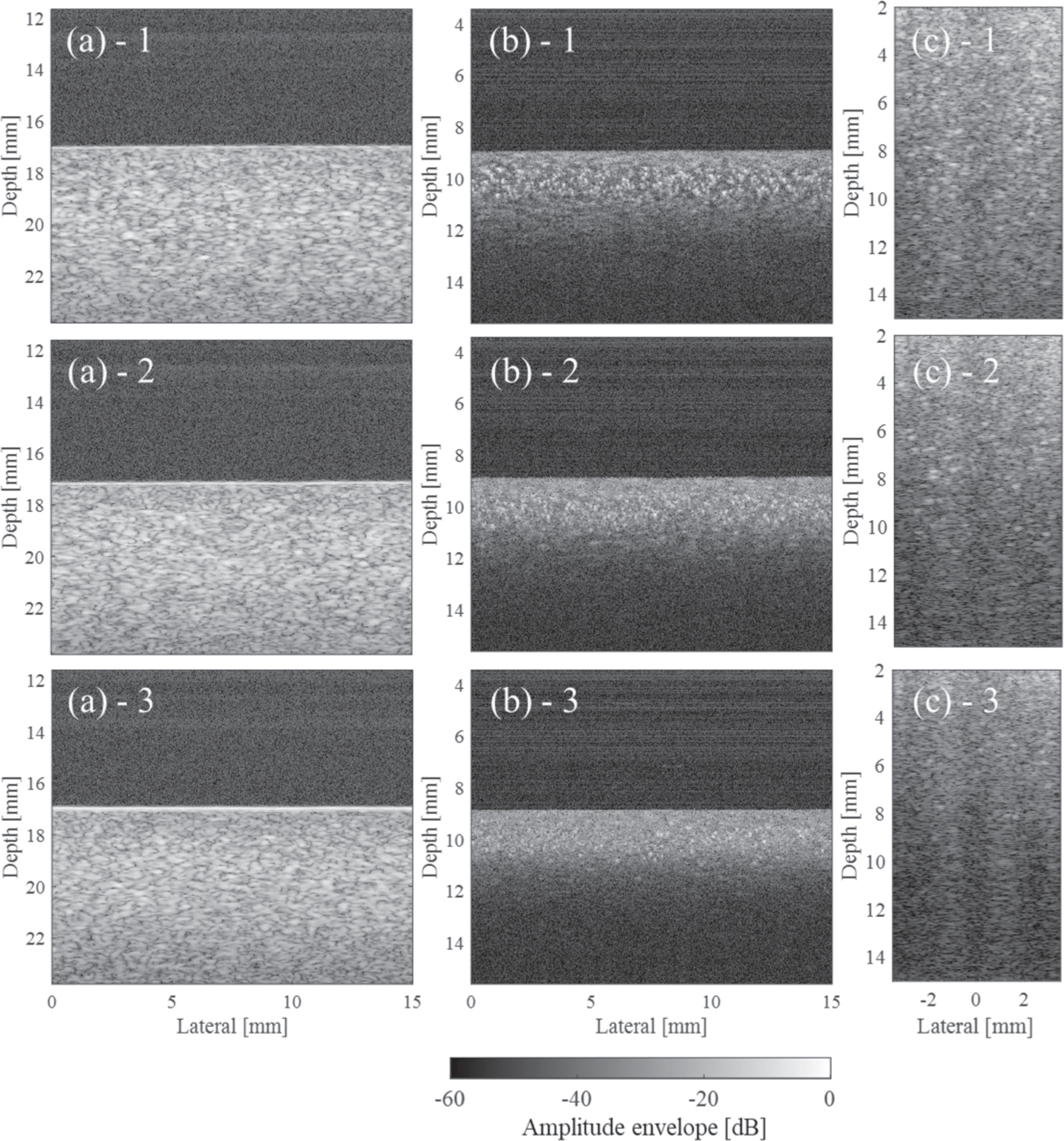
Fig. 10. B-mode images of (a-1)–(c-1) phantom D, (a-2)–(c-2) phantom F, and (a-3)–(c-3) phantom G acquired with (a) transducer I, (b) transducer II, and (c) the linear array probe.
Download figure:
Standard image High-resolution imageThe amplitude envelopes of phantoms D, F, and G obtained using transducer I, transducer II, and the linear array probe are shown in Fig. 11. The amplitude envelopes of phantoms A and B are also shown for comparison. The similarity of the signals acquired with transducer I for phantoms B, D, and F indicates that the strong scatterer was dominant in the reflected signal. The amplitude of the specular reflector was slightly higher because the speed of sound was higher in phantom G than in the other phantoms [Fig. 11(a)]. The signal intensities of phantoms B, D, F, and G acquired with transducer II were comparable, and the amplitude gradient of the signal below the focus became steeper as the number density increased owing to scattering attenuation [Fig. 11(b)]. Signals acquired with the linear array probe showed a higher scatterer number density but lower amplitude in phantom G than in phantoms B, D, and F. The comparison of phantoms B, D, and F suggests that the scattering intensities are not simply additive [Fig. 11(c)].

Fig. 11. Amplitude envelopes of phantoms A, B, D, F, and G acquired with (a) transducer I, (b) transducer II, and (c) the linear array probe.
Download figure:
Standard image High-resolution imageThe frequency spectra of phantoms A, B, D, F, and G acquired using each sensor are shown in Fig. 12. For transducer I, the frequency bandwidth tended to narrow as the number of weak scatterers increased [Fig. 12(a)]. For transducer II and the linear array probe, as in Figs. 7(b) and 7(c), the low-frequency signal increased with each increment in the scatterer number density, but the HF signal decreased owing to HF attenuation [Figs. 12(b), 12(c)].
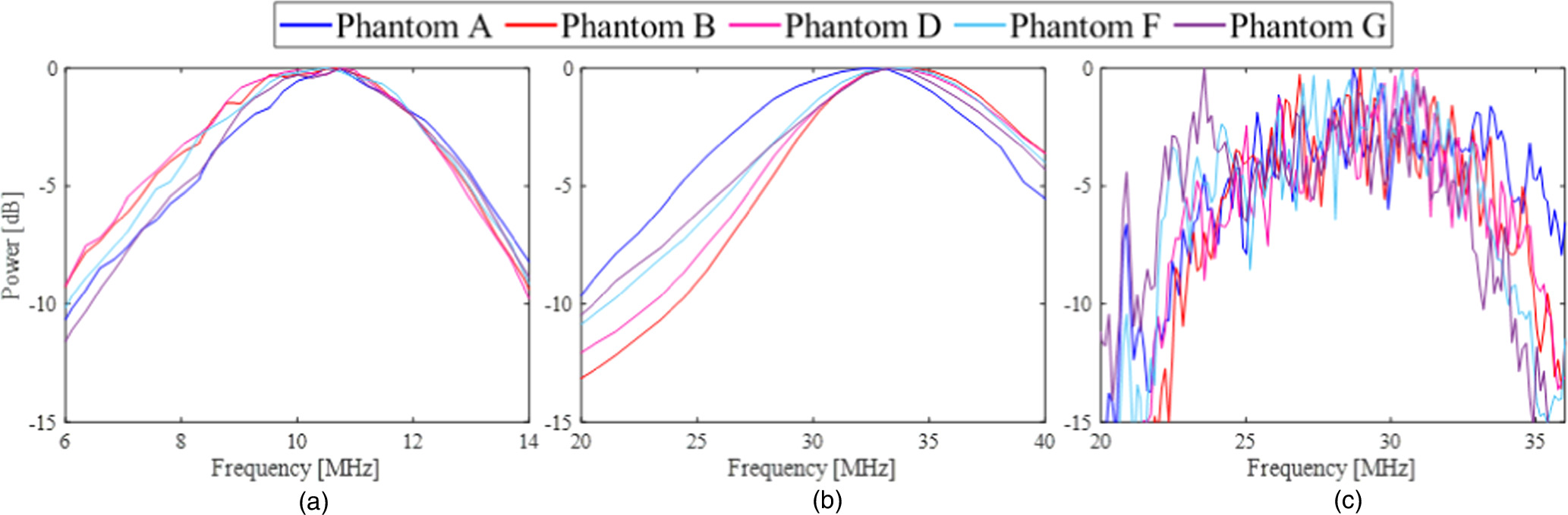
Fig. 12. Power spectrums of phantoms A, B, D, F, and G acquired with (a) transducer I, (b) transducer II, and (c) the linear array probe.
Download figure:
Standard image High-resolution imageThe estimated BSCs of phantoms D, F, and G acquired by each sensor and the theoretical values calculated using the mathematical model are shown in Fig. 13. The theoretical values for a phantom with two mixed scatterers were calculated in the same way as theoretical values were calculated in Sect. 3.2.1. The BSCs of phantoms B, D, F, and G were similar when measured using transducer I [Fig. 13(a)]. The deviation from the theoretical value was large when using transducer II, and similar results were obtained for phantoms B, D, and F. Phantom G had lower values than the other phantoms, and the difference was larger than the difference between the theoretical values [Fig. 13(b)]. In the measurements made with the linear array probe, as for the measurements made with transducer II, the deviation from the theoretical value was large but decreased as the scatterer number density increased. In addition, the frequency dependence was different in the frequency range from 25 to 35 MHz, where the slope became shallower as the number density increased [Fig. 13(c)].

Fig. 13. Backscatter coefficients of phantoms A, B, D, F, and G acquiredwith (a) transducer I, (b) transducer II, and (c) the linear array probe and theoretical values.
Download figure:
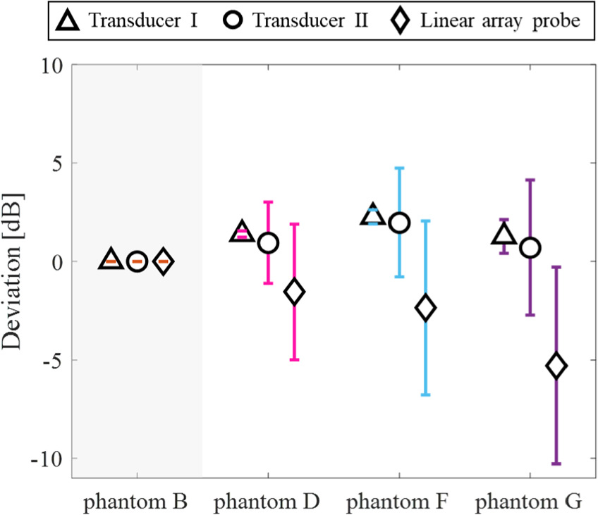
Standard image High-resolution imageThe deviation between the estimated BSC and the theoretical BSC obtained using the mathematical model is shown in Fig. 14. For all modalities, the mean value of the deviation decreased as the scatterer number density increased. The standard deviations of the deviations increased in the order of transducer I, transducer II, and the linear array probe.
Fig. 14. Deviations between the estimated backscatter coefficients for phantoms B, D, F, and G and the theoretical values calculated using the mathematical model.
Download figure:
Standard image High-resolution image
4. Discussion
In this study, the effects of the state of interference between different scatterers on backscattering characteristics were examined by changing the volume ratio of two types of scatterer. The amplitudes were evaluated for a medium with a fixed number of weak scatterers and an increasing number of strong scatterers and for a medium with a fixed number of strong scatterers and an increasing number of weak scatterers, as shown in Figs. 5(c) and 10(c). The amplitude remained low even in shallow areas as the number density increased owing to the weaker interference of the two types of scatterer. As shown in Figs. 5(a) and 10(a), the amplitudes of the specular echo from the water–phantom interface were similar, indicating that the acoustic impedances of the different phantoms were comparable. Overall, the agreement between the measured and theoretical BSCs was satisfactory in the frequency bandwidth of 6–12 MHz [Figs. 4(a), 8(a)]. However, the measured BSCs were appreciably different from the theoretical predictions at higher frequencies of 20–40 MHz [Figs. 4(b), 8(b)]. The curve of the BSC theoretical prediction had a dip at approximately 23 MHz and a sharp peak at approximately 27 MHz, whereas the measured BSC had a smooth curve. In this paper, the Faran model, which takes elastic waves into account, was applied to evaluate the phenomena observed in actual measurements, but the Faran model assumes that the surrounding medium is water and does not consider attenuation or elasticity in the medium. This discrepancy might explain the difficulty of capturing in experiment the wave propagation of elastic polystyrene spheres, which seem to be largely attenuated in ager gel. Further experimental studies are needed to make progress on this point by comparing the backscattering responses of elastic spheres suspended in water and those of elastic spheres in agar gel. The structure factor model expressed by Eq. (8) in Ref. 36, which does not take elastic waves into account, gives a smooth frequency dependence, which indicates the effect of elastic waves. The structure factor model does not match the evaluation results of the present study, with the frequency dependence and amplitude being different. Therefore, in this study, we adopted the Faran model, which is commonly used for backscattering coefficient evaluation, for comparison.
In the actual measurements, as shown in Figs. 8(b) and 13(b), the scattering from the strong scatterers was greater than that from the weak scatterers, and the signal from the strong scatterers was dominant in the two-scatterer mixed phantom. Therefore, the interference signal of the weak scatterers was small. In Fig. 8(c), the signal from strong scatterers in the analysis region was weakened by interference from the signal from surrounding weak scatterers, resulting in lower contrast, and the BSC amplitude was thus estimated to be small. This can be understood from the fact that both the slope and amplitude were smaller, as shown in Fig. 13(c). In other words, the result was due to the effect of weaker interference from strong scatterers and dominant signals from weak scatterers. In addition, under the conditions of this study, the effect of interference becomes more pronounced at higher frequencies.
Figures 9 and 14 show that the standard deviation of the deviation was larger for each increase in the number density of scatterers in the order of transducer I, transducer II, and the linear array probe, and the data acquired with the linear array probe had the largest deviation from the relation of the frequency dependence, indicating the effect of interference. The average deviations in the BSC estimation results for phantom E in Fig. 8(b) and phantom G in Fig. 13(b) are lower than the results for the other phantoms, indicating the influence of interference. However, this effect is smaller than that of the linear array probe. The standard deviation was small for transducer I, indicating that the frequency dependence of the deviation was highly consistent despite the difference in amplitude. Thus, interference between the two types of scatterer had an appreciable effect on the backscattering characteristics when evaluated with a high-intensity and HF sensor.
5. Conclusions
To understand the effect of wave interference generated by correlation among scatterer positions, we compared the backscattering characteristics of a phantom with a mixture of two types of scatterer using several sensors. The signal acquired with a single transducer showed only a weak effect of interference, whereas the signal acquired with a linear array probe of high intensity and HF showed a weak effect of interference that became more pronounced as the number density of scatterers increased. However, the scattering intensity of actual biological tissues differs appreciably from that of the simulated biological samples used in this study and has a more complex scatterer distribution, and it is presumed that the frequency dependence of the BSC will have more diverse variations. In future work, we will evaluate the scattering intensity of real biological tissues and that of media with a heterogeneous scatterer distribution and structure and thus a scattering intensity closer to that of biological tissues.
Acknowledgments
This work was partly supported by JSPS KAKENHI under grant no. 23H03758 and 22KK0179 and the Chiba University Institute for Advanced Academic Research. We thank Edanz (https://jp.edanz.com/ac) for editing a draft of this manuscript.