
Abstract
Rock type classification is crucial for evaluating mineral resources in ore deposits and for rock mechanics. Mineral deposits are formed in a variety of rock bodies and rock types. However, the rock type identification in drill core samples is often complicated by overprinting and weathering processes. An approach to classifying rock types from drill core data relies on whole-rock geochemical assays as features. There are few studies on rock type classification from a limited number of metal grades and dry bulk density as features. The novelty in our approach is the introduction of two sets of feature variables (proxies) at sampled data points, generated by geostatistical leave-one-out cross-validation and by kriging for removing short-scale spatial variation of the measured features. We applied our proposal to a dataset from a porphyry Cu–Au deposit in Mongolia. The model performances on a testing data subset indicate that, when the training dataset is not large, the performance of the classifier (a random forest) substantially improves by incorporating the proxy features as a complement to the original measured features. At each training data point, these proxy features throw light based on the underlying spatial data correlation structure, scales of variations, sampling design, and values of features observed at neighboring points, and show the benefits of combining geostatistics with machine learning.
Export citation and abstract BibTeX RIS

Original content from this work may be used under the terms of the Creative Commons Attribution 4.0 license. Any further distribution of this work must maintain attribution to the author(s) and the title of the work, journal citation and DOI.
1. Introduction
An economic mineral deposit that is termed an 'ore' deposit, is an unusually high concentration of metallic or non-metallic minerals in a part of the Earth's crust that can be extracted economically or strategically [1]. The identification of the rock types (lithology), ore-bearing geologic structures, and the geological properties of those rocks, are fundamental in defining ore deposits. Exploration geologists are initially concerned with the lithology of the country rocks, and subsequently move toward the identification of the host rocks (that host the ore body) and wall rocks (that surround the host rocks). Geological properties that characterize the different rock types in an ore deposit include the basic physical attributes that can be observed with the naked eye, and attributes pertaining to geochemistry, petrography, mineralogy, alteration, material science and rock mechanics which can be measured only in the laboratory. The classification of rock types is helpful to many modeling and engineering decisions in downstream stages of a mining project, such as: (1) generating geologic maps and 3D geological models, (2) estimating the probability of occurrence of economic minerals in a particular rock type, (3) estimating the cost of blasting and extracting the raw material to be mined, (4) adjusting drilling parameters for a given rock type to maximize core recovery, (5) estimating recoverable resources, and (6) estimating the rock strength, among others.
In practice, the visual determination of the rock type on the basis of its mineralogy (when distinct), color, grain size and texture, structure, contacts with other rock types, or other visual attributes, is the regular method of identifying and classifying a lithology. However, two rocks may look very much the same physically, but be geochemically different. When the visual procedure fails to exactly determine or confirm the lithology class, chemical assays of the rock samples reveal their exact type. However, chemical assays of rocks involve service costs that have to be planned judiciously.
Porphyry Cu deposits, including porphyry Cu–Au–Mo and porphyry Cu–Au deposits, and Cu–(Mo) breccia pipes are the world's largest source of copper. These are generally large-tonnage–low-grade metal deposits. Ore occurs in bulk-mineable mineralization that is spatially, temporally and genetically associated with intrusive rock plutons of the granite family with the metals transported by hydrothermal fluids [2]. The intrusive plutons, host or wall rocks, and other country rocks are commonly subjected to hydrothermal alteration overprinting, resulting in a loss of the original physical signature of the lithology types, thereby posing a difficulty in their visual identification and classification. Alteration caused by weathering and meteoric waters acidified after percolating through iron sulfides (pyrite, FeS2) in the deposit, further adds to the problem of labelling the exact rock type. This is the first dimension to the problem addressed here.
Where chemical assay of the rock sample is the available solution to the identification of the lithology, there lies another problem, related to the cost-benefit paradigm of the mining and metals industry. Why would a mining company invest money in assaying a population of rocks sampled from a lithologic domain if a few initial sample assays indicate a poor metal grade of the domain? This economic logic leads to the resultant problem of missing values of some or all assay variables pertaining to the rock sample at a data point in underground 3D space. This is the second dimension of the problem.
A more pessimistic corollary of the same logic adds a third and more acute dimension: complete absence of information. Why would the company invest at all in additional drill holes for extracting those cylindrical rock core samples from 'that' low-grade lithologic domain? A core loss or poor core recovery during drilling is an additional risk. The complete absence of information leads to 'no data' patches of underground zones among zones of 'data-rich' and 'data-poor' irregularities.
There are two perspectives on handling missing data: avoiding the rows in which some or all variables have missing values, versus filling the missing values by statistically calculated imputations. The former approach is naive, conservative, faithful to the missing values, but implies discarding a data point location along with grade values that are costly to acquire. The latter approach appears reasonable for most investigators but is considered as inappropriate practice by mineral resource reporting systems belonging to CRIRSCO [3]. It is pertinent to note that data imputation in the blank cells of the assay data table means imputing values of the components of a spatial vector at different data point locations, which implies changing the original spatial data configuration from 'partially heterotopic' (i.e. with under-sampled variables) to 'isotopic' (with equally-sampled variables).
One typically characterizes mineralization by sampling less than 0.001% of the deposit. Therefore, the scale of uncertainty combined with high levels of geological variability create unique risks for the profitable exploitation of mineral resources. The ultimate problem is that given a sparse population of rock core data at scattered locations, we are required to predict the spatial distribution of the different rock types and metal grades comprising the 3D subsurface of the deposit [4–6]. The traditional approach of classifying the rock type of drill core samples relies on whole-rock geochemical assays, comprising concentrations, and their transformed values, of a series of major oxides, alkaline and alkaline-earth elements, trace elements, and other elements to as much as 55–60 feature variables. While several machine learning case studies exist on rock type classification from whole-rock geochemistry (e.g. [7, 8]), there are perhaps just a few on rock type classification from a limited number of feature variables comprising essentially of assays of metal grades. This is primarily due to the general unavailability of proprietary drill hole datasets of ore deposits in the public domain for scientific research.
The prime novelty of our study is the ingenious introduction of two complementary sets of feature variables ('proxies') at sampled data points, by means of geostatistical techniques: (1) leave-one-out cross-validation (LOOCV), and (2) filtered kriging for removing short-scale spatial variation ('noise') of laboratory measured values. Relying on the different sets of feature variables—the original measured set and the two sets of proxies, we tested a machine learning technique, namely the Random Forests (RF) [9], in tandem for classifying a total of 13 rock types occurring within the ore deposit.
Our principal scientific questions in the current research investigation are:
- 1.Is it possible to predict (classify) the different rock types with reliable accuracy from a given set of assayed grade values at sampled data locations? Our intuition is based on that it could be possible using a machine learning classifier provided the classification algorithm can recognize a decisive pattern of numerical features (metal grades) associated with each individual rock type. The input 'features' are assay values of geochemical variables and bulk density (BD) measured in a drill hole dataset in compliance with industry quality assurance and quality control standards. We will assess the accuracy of predictions by evaluation with standard model performance metrics for classification.
- 2.Could the different rock types be predicted with more accuracy if we add complementary sets of numerical features (proxy grade values generated by geostatistical techniques) to the original assayed grade values? In this case, our intuition is based on that more accurate prediction is plausible as a more distinctive pattern of features could be likely generated corresponding to each individual rock type (thus, rendering the classifier as more efficient in recognizing the pattern). The underlying merit of the complementary sets of grade values is that they are spatially correlated with the original assayed grade values.
- 3.What could be the prediction performances of the classifier if we were to substitute the assayed grade values at the sampled data locations and the missing values by the complementary sets of features (proxy grade values) generated by geostatistical techniques?
While trying to answer the above questions, we will analyze two cases, depending on whether the feature variables are equally sampled or not; in the latter case, the missing data will be filled with the median value per lithology class for each corresponding input feature variable to apply the traditional classification approaches.
The paper is outlined as follows: section 2 provides a geological description of the application case study under consideration. The dataset of this case study is introduced in section 3, together with the proposed tools and methodology. Section 4 presents and discusses the results of the classification problem. Section 5 concludes the paper, while detailed statistics on the classification results are provided in Appendices.
2. Geologic setting of the deposit
Porphyry deposits are regionally associated with convergent plate boundaries, along island arcs and continental margins where subduction of oceanic crust takes place beneath continental crust. The mineralization process is characterized by intrusions of large volumes of granitic magma accompanied by the availability of metal-rich hydrothermal fluids, with the sites of ore localization controlled by structural features, rock types, and hydrothermal alteration styles. Copper and gold are typically the main economic minerals in these deposits, with molybdenum and silver being common as additional. A good summary of porphyry deposits, their types of metal associations, host rocks, and alteration can be found in [10]. The details of the ore-forming process can be found in [2, 11].
The Central Asian Orogenic Belt extends for 5000 km from the Urals in the west to the Pacific coast in the east. Within this belt, a chain of porphyry mineralization occurs in Uzbekistan, Kazakhstan, Russia, China, and Mongolia, ranging in age from the late Neoproterozoic till the Jurassic. The most prolific geologic period of ore formation, including the largest deposits, was during the Late Devonian and Early Carboniferous [12].
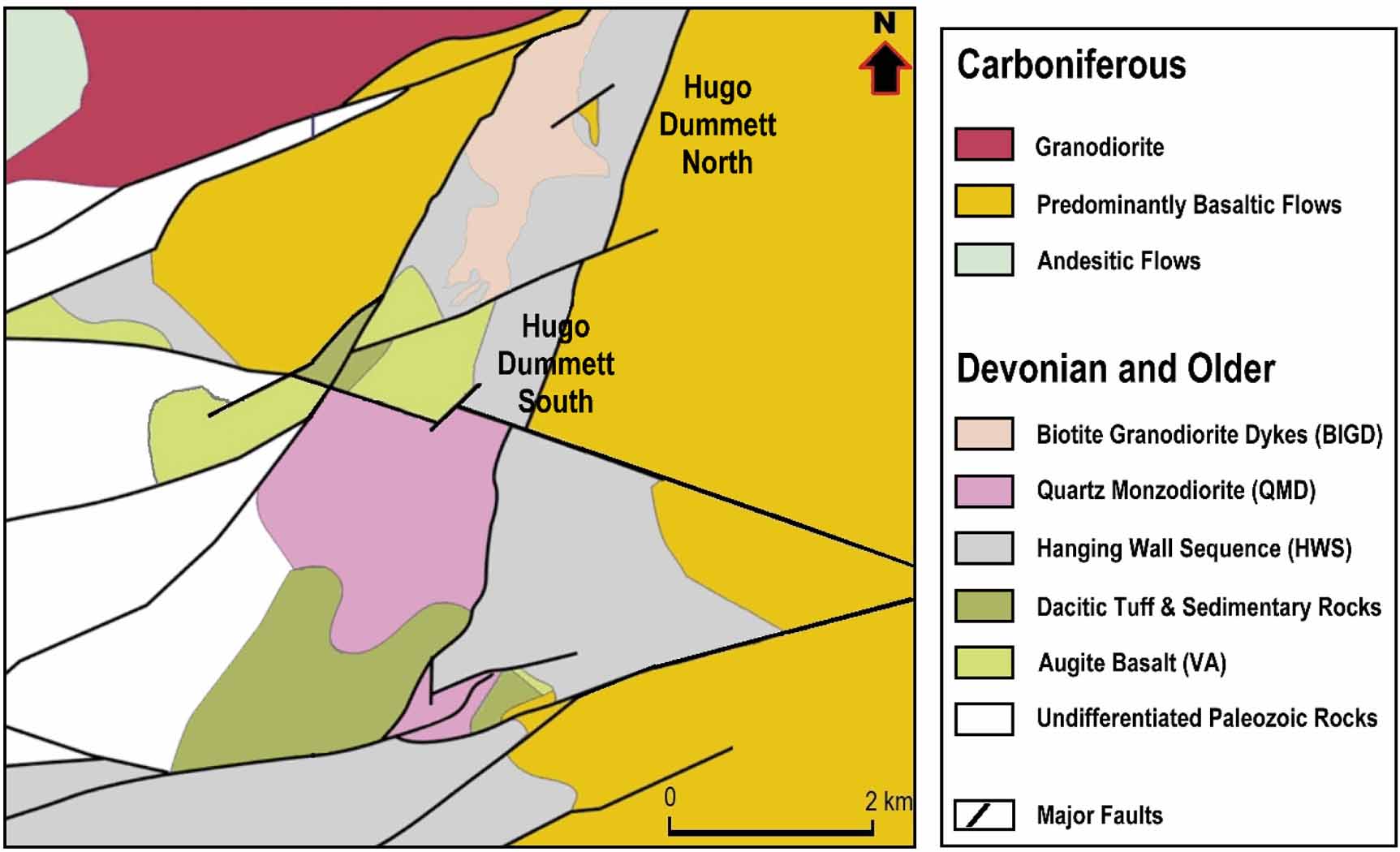
In Mongolia, porphyry mineralization occurs in two places: Erdenet and Oyu Tolgoi. Erdenet is located in Central Mongolia, whereas Oyu Tolgoi is located within the South Gobi Desert, approximately 650 km due south of the capital, Ulaanbaatar. The latter constitutes a cluster of seven porphyry Cu–Au–Mo–(+Ag) deposits, the largest high-grade group of Paleozoic porphyry deposits known in the world. The rock sequence surrounding this cluster of deposits is predominantly composed of basaltic to intermediate volcanic rocks of Devonian age, overlain by layered dacitic pyroclastic and sedimentary rocks intruded by basaltic and dolerite sills. The southern deposits (Southwest, Heruga North, and Heruga) are characterized by high Au (g/t)/ Cu (%) ratios (0.8-3:1), and hosted by biotite-magnetite-altered augite basaltic rocks. In contrast, the Hugo Dummett (North and South) deposits are characterized by lower Au (g/t)/ Cu (%) ratios (0.1-1:1), and hosted mainly by volcanic and plutonic rocks with extensive sericitic and advanced argillic hydrothermal alteration. The detailed geology and mineral exploration history in the Oyu Tolgoi district can be found in [13, 14].
The deposit concerned in this study is the Hugo Dummett South deposit (figure 1). It is a polymetallic porphyry with economic grades of Cu, Au, Mo and Ag and potentially deleterious grades of As, F, S and Fe. It is hosted by an east-dipping basalt rock sequence intruded by porphyritic quartz-monzodiorite plutons. The deposit is both disrupted by, and bounded by fault displacements in four directional orientations. The mineralization occurs in an anastomosing network of stockwork veinlets of sulfides ± quartz with Cu grades typically greater than 2%. There are potentially multiple overlapping mineralizing phases. Hydrothermal alteration exhibits a strong lithologic control with a number of assemblages including advanced argillic, muscovite/sericite, and intermediate argillic styles with minor K-silicate alteration. The stockwork is mainly localized within the Late Devonian quartz-monzodiorite intrusive; however, it also extends into the basaltic wall rock units.

Figure 1. Simplified geological map of the Hugo Dummett South porphyry deposit considered in this study and its surrounding area.
Download figure:
Standard image High-resolution image3. Materials and methods
3.1. Data description
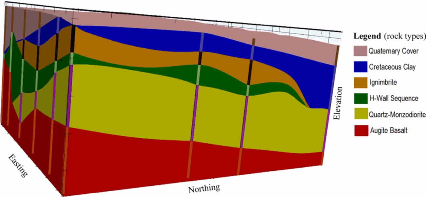
In the present study, we have considered an exploration dataset comprising geological, geochemical, and survey information of 360 drill holes representing 178 km of drilling. The dataset includes separate spreadsheets: assay values of thirteen chemical elements (Cu, Au, Ag, Mo, As, Fe, S, C, F, Pb, Zn, Cd, Hg), dry BD values, lithology classes, alteration types, mineral percentages, and survey data in the form of collar and down-the-hole survey files. In the original assay table, core sample lengths vary from 0.1 m to 1908.8 m (excluding the core loss intervals). Sample lengths in the range of 1 m – 3 m comprise 98.4% of the total samples. As per standard practice, samples were optimally composited to a mean length of 5.0 m without any left-overs, in lieu of fixed-length compositing. Decomposition of 12 large samples into smaller length composites has been done due to the fact that samples with lengths  m have negligible grade values for all the thirteen assay variables. Basic statistics on the target and feature variables are provided in tables 1 and 2, respectively. An interpretive lithological model (3D) with the trajectories of drill holes is shown in figure 2.

Figure 2. Interpretive lithological model (3D) used for mineral resource estimation with the drill hole intercepts superimposed. Coordinate values are omitted for confidentiality reasons.
Download figure:
Standard image High-resolution imageTable 1. Statistics on target variable (lithology) in composited data table.
| Serial number | Category | Code | Age | Number of records |
|---|---|---|---|---|
| 1 | Carboniferous andesite dyke | AND | Carboniferous | 1941 |
| 2 | Basalt dykes | BAD | Carboniferous | 4683 |
| 3 | Biotite granodiorite dykes | BIGD | Late Devonian and older | 7394 |
| 4 | Cretaceous clay | CLAY | Cretaceous | 1352 |
| 5 | Faults | FLT | Late Devonian and older | 1810 |
| 6 | Hydrothermal breccia | HBX | Late Devonian and older | 576 |
| 7 | Hanging wall sequence | HWS | Late Devonian and older |

|
| 8 | Ignimbrite | IGN | Late Devonian and older | 9181 |
| 9 | Carboniferous intrusive | INTR | Carboniferous | 160 |
| 10 | Quaternary cover | QCO | Quaternary | 13 |
| 11 | Quartz monzodiorite | QMD | Late Devonian and older |

|
| 12 | Carboniferous rhyolite dykes | RHY | Carboniferous | 2500 |
| 13 | Augite basalt | VA | Late Devonian and older | 6821 |
| Total |

|
Table 2. Statistics on assay variables in composited data table ( composites).
| Variable | Number of records | Number of missing values | Minimum | Maximum | Mean | Standard deviation |
|---|---|---|---|---|---|---|
| Cu (%) |

|

| 0.00 | 16.68 | 0.6049 | 0.7540 |
| Au (ppm) |

|

| 0.00 | 13.61 | 0.0858 | 0.2264 |
| Ag (ppm) |

|

| 0.00 | 32.17 | 1.2772 | 1.7289 |
| Mo (ppm) |

|

| 0.130 | 3007 | 44.32 | 65.08 |
| As (ppm) |

|

| 0.50 | 8416 | 134.09 | 301.87 |
| Fe (%) | 8299 |

| 0.26 | 16 | 4.3505 | 1.7195 |
| S (%) | 8320 |

| 0.00 | 18 | 1.9589 | 2.3614 |
| C (%) | 1362 |

| 0.01 | 14 | 0.4378 | 0.7892 |
| F (ppm) | 3994 |

| 12.8 |

| 1849.4 | 1907.7 |
| Pb (ppm) | 8299 |

| 1.91 | 3612 | 58.83 | 105.45 |
| Zn (ppm) | 8299 |

| 1.00 | 6936 | 223.42 | 360.63 |
| Cd (ppm) | 8299 |

| 0.00 | 30.43 | 0.6019 | 1.3849 |
| Hg (ppm) | 950 |

| 0.00 | 1.28 | 0.0953 | 0.1603 |
| BD (t/m3) |

|

| 2.30 | 2.89 | 2.7542 | 0.0433 |
3.2. Methods
3.2.1. Decision trees
A decision tree is a set of questions organized in a hierarchical manner and represented graphically as a tree, with a data structure made of a collection of nodes and edges, and devoid of loops. Nodes are divided into internal (or split) nodes and terminal (or leaf) nodes. All nodes have exactly one incoming edge. For a given input object, a decision tree predicts an unknown property of the object by asking successive questions about its known properties. Depending on the answer of a binary test, the data is sent to the right child node or to the left child node. This process is repeated until the data point reaches a leaf node. The leaf nodes contain a classifier or regressor which associates an output (a class label or a continuous value) with the input, and the decision is then made based on the output at the leaf node. The more the questions asked (the number of branches), the higher the confidence is in the response.
3.2.2. RFs
RFs [9] is an ensemble learning method that combines multiple decision trees to make predictions. It operates by constructing a collection (or forest) of decision trees, where each tree is trained on a subset of the training data. Randomness is introduced at two levels:
- 1.Bagging or bootstrap aggregating involves sampling the training data with replacement to create multiple bootstrap samples. Each decision tree is trained on a different bootstrap sample. This duplicates some samples and does not select others. An average of approximately 63.2% of cases is included in each training subset, whereas the remaining, or 'out-of-bag' (OOB) samples (approximately 37.8%) are used for validation.
- 2.Random feature selection: The second form of randomness involves selecting a random subset of features at each split node during tree construction. The number of variables in this subset is predefined and consistent across the forest. This feature subsampling helps to decorrelate the trees and to reduce overfitting. At every node, the randomly selected variables are then ranked by their ability to produce a split threshold that maximizes the homogeneity of child nodes relative to the parent node.
The class assigned by RF to each sample is determined by a majority vote combined from the prediction output of all classification trees. The reader is referred to [9, 15, 16] for the theory, mathematical rigor and consistency proofs of the algorithm, parameter selection, resampling mechanisms, variable importance measures, and the theoretical and methodological progress made since its initial development. Although RF has been extremely successful as a generic classification and regression method, it is routinely used for classification problems (e.g. [17–19]).
3.2.3. Kriging
Kriging is a geostatistical predictor that applies to a regionalized variable, i.e. a quantitative variable indexed by spatial coordinates. It relies on the modeling of the spatial correlation structure of this variable, via mathematical tools such as the (auto)covariance function or the variogram that quantify the similarity or the dissimilarity between paired observations of the variable, as a function of their spatial separation. Unlike machine learning techniques (e.g. decision trees or RFs) that are used to predict one variable (target) from another (feature), kriging predicts the same variable as the input, but at different spatial locations, with the unbiased prediction leading to the smallest mean-square error, i.e. the error with zero mean and the smallest variance. The reader is referred to [20] for details on the representation of regionalized variables by spatial random fields, inference and modeling of covariance functions or variograms, as well as on the mathematical background and the most common variants of kriging.
In the following section, two kriging-based approaches will be used to complement the original feature variables inputted in machine learning algorithms. The motivation is to account not only for the feature variables observed at a sampling location when predicting a target variable at this particular location, but also for the information brought by the feature variables observed at surrounding locations. These are:
- 1.LOOCV. The value of a feature variable at a given location is predicted by kriging, using as input the values of the same feature variable at surrounding locations and a modeled covariance function or variogram. The cross-validated prediction therefore includes the information of the neighboring data, but excludes the information of the data itself.
- 2.Kriging with filtering. This variant applies when the modeled covariance function or variogram of the feature variable is decomposed into two components; typically, the first component is the nugget effect variance, which stands for the discontinuity of the covariance function or variogram at the origin, while the second component is the continuous part of the covariance function or variogram. In such a situation, the feature variable can also be interpreted as the sum of two components, associated with the components of its covariance function or variogram. In particular, the nugget effect component represents the short-scale variability and noise associated with measurement errors [21], while the continuous component represents the spatial variations at larger scales. Kriging with filtering [22, chapter 15] allows predicting the continuous component of a feature variable (viewed as the 'error-free' variable) at a given location, using as input the values of the observed variable (including the nugget effect component) at this location and surrounding locations, as well as the modeled covariance function or variogram of the variable. Unlike LOOCV, here the prediction not only includes the information of the neighboring data, but also the information of the data itself.
3.3. Proposed methodology
The proposed methodology is illustrated in figure 3 and detailed in the next subsections. The objectives of this methodology are the following:
- 1.To test whether it is possible to predict different classes of intrusive lithology ('target variable') with assay variables and BD as input 'feature variables'. In doing so, our emphasis is not to test multiple machine learning algorithms for evaluating their individual predictive powers, but to, primarily, find out whether a limited number of assayed metal grades exhibit extractable patterns of variations for correlation with different rock types via supervised learning.
- 2.To compare classification performances by the traditional approach versus our ingenious approach of creating proxy variables as input features, as explained below. In the case where feature variables are not equally sampled, the traditional approach relies on imputing missing values. Although we had several statistical options of imputation, we opted for a geochemically sound procedure, i.e. the missing values were filled with the median value per rock type for each corresponding measured variable, to apply the traditional classification approach. The principal objective was to test whether the proxy variables created by us are: (a) indispensable, or (b) somewhat useful, or (c) useless, for the purpose of the said classification.

Figure 3. Schematic workflow of the proposed methodology, combining geostatistical analyses (yellow panel) and machine learning (green panels) for enhanced classification in a spatial context.
Download figure:
Standard image High-resolution image3.3.1. Geostatistical modeling of feature variables
The first step of the methodology is the calculation of experimental variograms to identify the spatial correlation structure of the feature variables (chemical element assays and BD), which encompasses their spatial variability at both short and large scales and can depend on the spatial direction. To avoid over-simplifications and to get a realistic geostatistical model, we considered two directions for variogram calculation: the horizontal plane (omni-horizontal calculations) and the vertical direction (table 3).
Table 3. Parameters for experimental variograms.
| Horizontal direction | Vertical direction | |
|---|---|---|
| Azimuth (°) | 0 | 0 |
| Azimuth tolerance (°) | 90 | 90 |
| Dip (°) | 0 | 90 |
| Dip tolerance (°) | 20 | 20 |
| Lag (m) | 15.0 | 10.0 |
| Number of lags | 20 | 20 |
| Lag tolerance (m) | 7.5 | 5.0 |
The fitting of theoretical variogram models considers nested structures of nugget, spherical and exponential types. The fit is performed with a least-square procedure (table 4 and figure 4).

Figure 4. Examples of variograms for chemical assays (Cu, Ag, As, Fe and S) and bulk density (BD). Crosses represent experimental variograms and solid lines represent fitted models, along the horizontal (black) and vertical (blue) directions.
Download figure:
Standard image High-resolution imageTable 4. Parameters for theoretical variogram models.
| Feature variable | Structure | Horizontal range (m) | Vertical range (m) | Partial sill |
|---|---|---|---|---|
| Au | nugget | 0 | 0 | 0.0049 |
| spherical | 20 | 150 | 0.0184 | |
| spherical | 200 |

| 0.0138 | |
| Cu | exponential | 20 | 150 | 0.3383 |
| exponential | 200 | 250 | 0.1793 | |
| exponential | 200 |

| 0.0429 | |
| Ag | nugget | 0 | 0 | 0.2035 |
| exponential | 10 | 20 | 0.3861 | |
| spherical | 40 | 130 | 1.4489 | |
| As | exponential | 10 | 20 |

|
| spherical | 25 | 160 |

| |
| C | exponential | 70 | 10 | 0.1232 |
| exponential | 150 | 20 | 0.1075 | |
| spherical |

| 200 | 0.1435 | |
| F | nugget | 0 | 0 |

|
| exponential | 150 | 70 |

| |
| Fe | nugget | 0 | 0 | 0.5656 |
| exponential | 40 | 40 | 1.5007 | |
| spherical | 100 | 100 | 0.7857 | |
| spherical | 100 |

| 0.0238 | |
| Mo | nugget | 0 | 0 | 1982.3 |
| exponential | 150 | 10 | 1250.7 | |
| exponential | 250 | 150 | 982.2 | |
| S | nugget | 0 | 0 | 0.8027 |
| exponential | 70 | 70 | 0.2095 | |
| exponential | 200 | 70 | 3.6043 | |
| Pb | exponential | 40 | 40 | 4539.1 |
| spherical | 100 | 100 | 2627.6 | |
| spherical | 100 |

| 5384.0 | |
| Zn | exponential | 50 | 20 |

|
| exponential | 130 | 130 |

| |
| Cd | exponential | 50 | 20 | 1.0198 |
| exponential | 130 | 130 | 0.6007 | |
| Hg | nugget | 0 | 0 | 0.0152 |
| exponential | 40 | 20 | 0.0107 | |
| spherical |

| 100 | 0.0086 | |
| BD | exponential | 20 | 250 | 0.00083 |
| exponential | 20 |

| 0.00013 |
3.3.2. Geostatistical prediction by LOOCV and kriging with filtering
For both types of prediction, the feature variables were kriged separately. In each case, ordinary kriging was used, with a moving neighborhood implementation. The shape of the neighborhood was ellipsoidal, and its anisotropy was chosen as a function of the anisotropy of the variogram model (e.g. the neighborhood was more elongated in case of a strong anisotropy, or closer to a sphere in case of isotropy) (table 5). To avoid getting predictions that are locally very high, a top-cut value was applied to feature variables with long-tailed histograms. Finally, to avoid inconsistent results, negative predictions were post-processed and set to zero.
Table 5. Parameters for kriging.
| Feature variable | Horizontal search radius (m) | Vertical search radius (m) | Optimal number of data | Top-cut value |
|---|---|---|---|---|
| Au | 1500 | 2500 | 40 | 2.0 ppm |
| Cu | 1500 | 2500 | 40 | 8.0 pct |
| Ag | 1500 | 2500 | 40 | 20 ppm |
| As | 1500 | 2500 | 40 | 5000 ppm |
| C | 8000 | 4000 | 40 | 10 pct |
| F | 2500 | 1500 | 40 |
 ppm ppm |
| Fe | 8000 | 7000 | 40 | |
| Mo | 2500 | 1500 | 40 | 500 ppm |
| S | 2500 | 1500 | 40 | |
| Pb | 8000 |

| 40 | 1500 ppm |
| Zn | 1500 | 1200 | 40 | 4000 ppm |
| Cd | 1500 | 1200 | 40 | 15 ppm |
| Hg | 8000 | 4000 | 40 | |
| BD | 1500 | 2500 | 40 |
3.3.3. Feature engineering
To compare the model performances corresponding to the traditional machine learning approaches versus our approach, we have created an extended dataset comprising of three sets of feature variables. The first set consists of the assay variables of the original dataset, i.e. Cu, Au, Ag, Mo, As, Fe, S, C, F, Pb, Zn, Cd, and Hg, plus BD. The second set consists of leave-one-out cross-validated ('LOOCV') values, and the third set consists of filtered (after removing the 'nugget variance' from the variogram) kriging values for each of the above feature variables. Only the first set contains missing values. In the third set, if the variable has no nugget, then the filtered value is equal to the original value; if the value of a variable is missing, then the filtered value is its kriging prediction from the surrounding values and matches the LOOCV value.
3.3.4. RF prediction (classification) of lithology classes
The following steps were performed sequentially.
Classification based on the dataset with imputed values (Models M1, M2 and M3)
- 1.The missing values of the first set of feature variables: assayed grade variables, viz., Cu, Au, Ag, Mo, As, Fe, S, C, F, Pb, Zn, Cd, and Hg, plus BD, were filled with the median value corresponding to each lithology class.
- 2.Our first task was to test the prediction of the lithology types with the first set of feature variables (14). Then, the next is to test the same combining the first, second, and third set of feature variables (
 feature variables). The last task is to test the same combining only the second and third set of feature variables ( feature variables). Statistics on the target variable (lithology) in the composited dataset is given in table 1. The dataset has 67 323 observation points, including imputed values for the first set of feature variables (14). We split the dataset into subsets comprising training and testing in a 70:30 ratio. Since lithology has been sampled in an unbalanced way, subsets comprising training and testing data were split through stratified random sampling. The prior probabilities are considered so as to match total sample frequencies (table 6). The purpose of sub setting the training rows is for model training and tuning, and the testing rows for model evaluation. Optimizing RF for modeling involves tuning some parameters controlling the structure of each individual tree, the structure and size of the forest as well as its randomness. The methodology and software that we have adopted for tuning hyperparameters for the RF classification models are described later in this section.


Table 6. Multi-class response information in the training and testing subsets.
| Lithology class | Prior | Training count | % | Testing count | % |
|---|---|---|---|---|---|
| AND | 0.02 | 1359 | 2.02 | 582 | 0.87 |
| BAD | 0.05 | 3279 | 4.87 | 1404 | 2.09 |
| BIGD | 0.08 | 5176 | 7.69 | 2218 | 3.30 |
| CLAY | 0.01 | 947 | 1.41 | 405 | 0.60 |
| FLT | 0.02 | 1267 | 1.88 | 543 | 0.81 |
| HBX | 0.01 | 404 | 0.60 | 172 | 0.26 |
| HWS | 0.17 |

| 16.67 | 4808 | 7.14 |
| IGN | 0.09 | 6427 | 9.55 | 2754 | 4.09 |
| INTR | 0 | 112 | 0.17 | 48 | 0.07 |
| QCO | 0 | 10 | 0.02 | 3 | 0.00 |
| QMD | 0.15 |

| 15.46 | 4459 | 6.62 |
| RHY | 0.03 | 1750 | 2.60 | 750 | 1.12 |
| VA | 0.07 | 477 | 7.09 | 2046 | 3.04 |
| All | 0.70 |

| 70.01 |

| 29.99 |
Classification based on the dataset without missing values (Models M4, M5 and M6)
- 2.Next, we repeat the exercise (prediction of lithology types with the RF classifier), but with all missing data (i.e. imputed values) removed. A reduction in the number of data points from to 899, and the number of lithology classes from 13 to 12 (table 7) was implicit due to the fact that missing values for different grade variables in the original dataset were not uniformly distributed among the data points. Dry BD (t m−3), a physical variable, in the dataset was discarded due to missing values at a huge proportion of these 899 data points. Hence, this time, the sets of feature variables consisted of only chemical grade variables: the first set consisted of 13 assayed chemical grade variables; the second set consisted of 13 cross-validated (LOOCV) chemical grade variables, and third set consisted of 13 kriged chemical grade variables with nugget effect filtering.
- 4.Due to the similarity in age and mode of formation, we merged the AND, RHY, and INTR lithology classes into a single class: INTR. Hence, the total number of lithology classes was reduced to 10 for this set of classification models. The final statistics of the lithology variable used for the prediction models are shown in table 8. For this set of models, we split the 899-point dataset into training/testing subsets in a ratio 70:30. Table 9 shows the number and percentages of lithology class records in the training and testing subsets.

Table 7. Multi-class response information (before merging) in the training and testing subsets.
| Serial number | Category | Code | Number of records |
|---|---|---|---|
| 1 | Carboniferous andesite dyke | AND | 17 |
| 2 | Basalt dykes | BAD | 40 |
| 3 | Biotite granodiorite dykes | BIGD | 34 |
| 4 | Cretaceous clay | CLAY | 14 |
| 5 | Faults | FLT | 107 |
| 6 | Hydrothermal breccia | HBX | 20 |
| 7 | Hanging wall sequence | HWS | 74 |
| 8 | Ignimbrite | IGN | 132 |
| 9 | Carboniferous intrusive | INTR | 1 |
| 10 | Quartz monzodiorite | QMD | 374 |
| 11 | Carboniferous rhyolite dykes | RHY | 66 |
| 12 | Augite basalt | VA | 20 |
| Total | 899 |
Table 8. Multi-class response information (after merging) in the training and testing subsets.
| Serial number | Category | Code | Number of records |
|---|---|---|---|
| 1 | Basalt dykes | BAD | 40 |
| 2 | Biotite granodiorite dykes | BIGD | 34 |
| 3 | Cretaceous clay | CLAY | 14 |
| 4 | Faults | FLT | 107 |
| 5 | Hydrothermal breccia | HBX | 20 |
| 6 | Hanging wall sequence | HWS | 74 |
| 7 | Ignimbrite | IGN | 132 |
| 8 | Carboniferous intrusive | INTR | 84 |
| 9 | Quartz monzodiorite | QMD | 374 |
| 10 | Augite basalt | VA | 20 |
| Total | 899 |
Table 9. Multi-class response information of table 8 separated into training and testing subsets.
| Lithology class | Training count | % | Testing count | % |
|---|---|---|---|---|
| BAD | 28 | 3.11 | 12 | 1.33 |
| BIGD | 24 | 2.67 | 10 | 1.11 |
| CLAY | 10 | 1.11 | 4 | 0.44 |
| FLT | 75 | 8.34 | 32 | 3.56 |
| HBX | 14 | 1.56 | 6 | 0.67 |
| HWS | 52 | 5.78 | 22 | 2.45 |
| IGN | 93 | 10.34 | 39 | 4.34 |
| INTR | 59 | 6.56 | 25 | 2.78 |
| QMD | 262 | 29.14 | 112 | 12.46 |
| VA | 14 | 1.56 | 6 | 0.67 |
| All | 631 | 70.19 | 268 | 29.81 |
Following the model runs for the above cases, we analyzed the model performances from each confusion matrix after deriving the accuracy rates, kappa statistics, and other statistics that include the sensitivity, specificity, precision, recall, prevalence, detection rate, and balanced accuracy. We also investigated the relative feature importance according to statistical criteria. Finally, we did some model tuning to make the models run on the testing subsets, for each of the three sets of feature variables, and obtain the final sets of results, which are reported in the Results section and in Appendices.
The randomForest R package version 4.7-1.1 [23], which implements Breiman and Cutler's RFs for classification and regression supporting the original Fortran code [9], was the fundamental package used to obtain the RF models. We, by and large, followed [24], for the parameter tuning strategies for the RF classification. The specific hyperparameter values were determined using the tuneRanger R package version 0.14.1 [25] that tunes the RF classifier using the OOB observations.
3.3.5. Hyperparameter tuning
We considered the following hyperparameters for tuning: (a) the number of candidate feature variables considered at each split (denoted as mtry), (b) number of observations that are drawn for each tree (i.e. sample size, denoted by n), and (c) the minimum number of observations in a leaf node (nodesize). An optimal compromise between low correlation and reasonable strength of the trees can be controlled by tuning the parameters mtry, n, and nodesize [9]. However, prior to tuning these three hyperparameters, we also estimated the hyperparameter ntree (number of trees to grow) by finding the optimal number of trees to grow using the R package of [23]. Resampling during model tuning was performed by 5-fold cross-validation. We used the tuneRanger R package, to choose the optimal hyperparameter values for our models. A default nodesize parameter value of 1 was used for all the models. The default splitting rule used was that minimizing the Gini impurity. Research on tuning hyperparameters for variable importance is still in its infancy [24]. Therefore, we report (see appendices) both measures of variable importance: the Gini variable importance (mean decrease Gini) as well as the permutation variable importance (mean decrease accuracy).
4. Results and discussion
4.1. Performances of classification models
The optimally tuned model was selected based on the highest accuracy of candidate models with different hyperparameter values. The accuracy rate was computed using predictions made using the optimized model on the training dataset. The final hyperparameter values used for models M1, M2, M3, M4, M5, M6 and their prediction performances are indicated below (tables 10 and 11). Additional results are tabulated in appendix
Table 10. Prediction performance for models based on dataset with imputed values.
| Model = M1 | Model = M2 | Model = M3 |
| 14 predictors | 42 predictors | 28 predictors |
| (Assay: 14) | (Assay: 14 + LOOCV: 14 + Filtered-K: 14) | (LOOCV: 14 + Filtered-K = 14) |
| Target: Lithology classes = 13 | Target: Lithology classes = 13 | Target: Lithology classes = 13 |
| Hyperparameters | Hyperparameters | Hyperparameters |
| mtry = 12 | mtry = 24 | mtry = 2 |
| ntree = 250 | ntree = 400 | ntree = 500 |
| splitrule = gini | splitrule = gini | splitrule = gini |
| minimum node size = 1 | minimum node size = 1 | minimum node size = 1 |
| Training set = 47 131 samples | Training set = 47 131 samples | Training set = 47 131 samples |
| Accuracy = 99.61% | Accuracy = 99.64% | Accuracy = 99.64% |
| Testing set = 20 192 samples | Testing set = 20 192 samples | Testing set = 20 192 samples |
| Accuracy = 99.61% | Accuracy = 99.65% | Accuracy = 82.02% |
| Kappa = 0.9954 | Kappa = 0.9958 | Kappa = 0.7854 |
Table 11. Prediction performance for models based on dataset without missing values.
| Model = M4 | Model = M5 | Model = M6 |
| 13 predictors | 39 predictors | 26 predictors |
| (Assay: 13) | (Assay: 13 + LOOCV: 13 + Filtered-K: 13) | (LOOCV: 13 + Filtered-K = 13) |
| Target: Lithology classes = 10 | Target: Lithology classes = 10 | Target: Lithology classes = 10 |
| Hyperparameters | Hyperparameters | Hyperparameters |
| mtry = 7 | mtry = 20 | mtry = 2 |
| ntree = 250 | ntree = 200 | ntree = 450 |
| splitrule = gini | splitrule = gini | splitrule = gini |
| minimum node size = 1 | minimum node size = 1 | minimum node size = 1 |
| Training set = 631 samples | Training set = 631 samples | Training set = 631 samples |
| Accuracy = 80.19% | Accuracy = 100% | Accuracy = 100% |
| Testing set = 268 samples | Testing set = 268 samples | Testing set = 268 samples |
| Accuracy = 61.19% | Accuracy = 67.54% | Accuracy = 67.16% |
| Kappa = 0.4869 | Kappa = 0.5669 | Kappa = 0.5611 |
4.2. Discussion
Need for spatial machine learning
RF is a machine learning tool that has proved to be useful in doing regression and classification analyses. However, RF was not developed for modeling spatial stochastic processes because of its inherent inability to take into account the nature of spatial dependency (the spatial autocorrelation structure) intrinsic to such processes. However, there have been attempts made for spatial prediction (regression) using alternate models or even integrating RF with geostatistical algorithms. Notable are that of spatial linear mixed-models [27], RF-GLS [28], RF-Residual Kriging [29, 30], spatial RF [31] and geographical RF [32]. The spatial structure intrinsic to mineralization can extend to nested structures with additional difficulties of modeling spatial drifts with estimation complexities [20, 22], in the events of which the above-cited modeling frameworks, unfortunately, fall short in theory. In particular, when grades of core-samples are the input data to obtain predictions of average grades of unit blocks with volumes different from that of the core-samples, the problem of 'change of support' [20] is invoked, which a unique contribution of geostatistics in the realm of stochastic processes.
The scientific problem in this investigation does not necessitate to merge the algorithms of RF with those of geostatistics. At first glance, the problem is simply one of classifying the likely rock type associated with a given spatial pattern of grade variations measured on drill cores. However, there are additional dimensions to the problem, as cited in section 1, making it more complex. The traditional method for missing values in a dataset is to impute with realistic values. Then arises, which value is realistic and which is not? This is where expert subject knowledge comes in. Notwithstanding this, we approached the missing data problem with the simplest technique, that is, imputing the missing values by the median grade per lithology type. On the other hand, we have the option of incorporating proxy variables with values at each data point generated by geostatistics. Hence, the task was to evaluate which technique—traditional versus geostatistical—is superior.
Incorporation of spatial information in classification by geostatistics
The large amount of data and feature variables used in the first exercise that considers the dataset with imputed values leads to accuracy rates close to 100% (table 10). However, this performance significantly decreases when reducing the number of data and feature variables to the subset of data with no missing values (table 11), in which case the traditional RF classifier (model M4) applied to the testing dataset reaches an accuracy of 61.2% only and a kappa statistic less than 0.49. In this case, the prediction performances of model M5, for which the accuracy raises to 67.5% and the kappa statistic to 0.56, show the importance of incorporating proxy variables obtained by a spatial processing of the input information:
- The LOOCV predictors convey information on the expected value of the feature variables at an observation point, based on the spatial correlation structure of these variables, on their sampling design and on their values observed at neighboring points. Because they ignore the values at the target observation point, these LOOCV predictors can be seen as a 'summary' of the neighboring information at the point under consideration.
- The filtered kriging predictors provide another complementary information, consisting of the expected values of the feature variables if there were no short-scale variability or measurement errors. If one decomposes the feature variables into a 'signal' (associated with the continuous component of the covariance function or variogram models) and a 'noise' (associated with the nugget effect), the kriging with filtering provides a predictor of the former, i.e. the noise-free feature variables. As the LOOCV, this predictor accounts for the spatial correlation structure of the feature variables, their sampling design and their values observed at neighboring points, but also for the value observed at the target point, which is not 'wasted' as in LOOCV, and for the basic nested structures used in the spatial correlation model, which are associated with different scales of variations [22]. The rationale of using the filtered kriging predictors is that the relationship between the lithology (output) and the feature variables (input) is better explained by considering the large-scale variations of the inputs that are not contaminated by short-scale variations. This is analogous to the denoising of images with convolutional neural networks [33], except that it is applicable even when the observations are not arranged in a regular sampling design. Note that, if the correlation model does not have a nugget effect, then the filtered kriging predictor matches the original predictor at any point where the latter is observed.
Another significant advantage of using the LOOCV and filtered kriging predictors in the classification problem is the handling of missing data, insofar as they provide a 'clever' alternative to the imputation of missing values, based on the spatial correlation structure and neighboring information, instead of (in complement of) a simple median value by lithological class. The use of geostatistical proxies can be decisive in the presence of highly heterotopic datasets, for which discarding the missing data would imply a considerable loss of information. Note that the LOOCV and filtered kriging give the same predicted value for a feature variable at a point with missing observation.
Associations between lithology and chemical assays
Minerals and metal enrichments in porphyry ore deposits are formed by the precipitation of sulfides from a hydrothermal system accompanying magma intrusion through pre-existing host rocks. Several interrelated phenomena get activated during such ore-forming processes, which depend on the geochemical, petrophysical (e.g. porosity, permeability) and thermodynamical (pH, redox potential, thermal conductivity, etc) rock properties, and on the environment of magma generation and its chemical characteristics.
Some chemical elements are more likely to be found in specific rock types than in others in the Earth's crust [34]. However, this usual metal-rock associations based on geochemical affinity may change once a mineralization event takes place. As in our case, elements such as Cu, Zn, and Au (both chalcophile and siderophile) have got hosted both in an intrusive acidic igneous rock such as quartz-monzodiorite (QMD), as well as in the basic igneous wall rock such as Augite Basalt (VA), after the hydrothermal mineralization event.
Accordingly, an explicit quantitative assessment of the lithology-grade relationship is a very arduous task. To top it all, grade assays are affected by short-scale geological variability and measurement errors, which renders their relationship with the lithology 'noisier' and more difficult to display.
Our work suggests that machine learning classification can successfully model this complex lithology-grade relationship and predict the lithology from the grade assays, and even better when the spatial information is taken into consideration, in particular when different scales of spatial variations are identified and the short-scale variability of the grade assays is filtered out.
Variable importance in the classification models
Bootstrap aggregating (bagging) is a general-purpose procedure for reducing the variance of a statistical learning method. When we perform bagging involving many trees, it is no longer possible to represent the resulting statistical learning method using a single tree, and it is no longer clear which variables are most important to the procedure. Thus, bagging improves prediction accuracy at the expense of interpretability. However, we can obtain an overall summary of the importance of each predictor using the Gini index. This index is a measure of node purity—a small value indicates that a node contains predominantly observations from a single class. We add up the total amount that the Gini index is decreased by splits over a given predictor, averaged over all bagged trees.
The RF algorithm estimates the importance of a variable by looking at how much prediction error increases when (OOB) data for that variable is permuted while all others are left unchanged. The necessary calculations are carried out tree by tree as the RF is constructed [35]. There are actually four different measures of variable importance implemented in the original code. However, we report only two measures of variable importance in appendix
In the results, models M2 and M5 comprise the three sets of predictors: (1) original assayed grades (denoted with the index 1 in the Appendices, e.g. Cu1, Au1, Ag1), (2) LOOCV predictors (denoted with the index 2), and (3) filtered kriging predictors (denoted with the index 3). Model M2 constitutes the data table when the original assayed grades are imputed by the median value per lithology at the missing data points. Model M5 constitutes the data table with those data points, at which missing data occurs, completely removed. We can see in appendix
Despite this fact, the lower performance of model M3 in comparison with models M1 and M2, and the marginally lower performance of model M6 in comparison with model M5, show that, even if they are the most important, the LOOCV and filtered kriging predictors are a complement to, not a substitute of, the original assayed predictors.
5. Concluding remarks
This work fits into the context of mineral resources modeling and dealt with the use of machine learning to predict lithological classes from a set of feature variables (geochemical elements and dry BD), through a case study of a polymetallic porphyry deposit located in Mongolia.
Classification has been performed with the RF algorithm. Our main finding is that, when the training set is not so large, the predictive performance of RF can be substantially improved by incorporating new feature variables corresponding to proxy variables calculated by the geostatistical technique of kriging. Specifically, two proxies have been introduced, consisting of (1) LOOCV predictors that summarize, at each data location, the information of its neighboring data, and (2) the filtered kriging predictors that provide a denoised version of the feature variables, which carries out information on the continuous components of the feature variables, free of measurement errors. The proxy variables calculated at a data point account for the spatial data correlation structure, scales of variations, sampling design, and values of the features observed at neighboring points. In the second classification exercise (with 631 data in the training set and 13 feature variables), the accuracy rate on the testing dataset raised from 61.2% without the proxy variables, to 67.5% with these variables.
Another advantage of using geostatistical proxy variables is the possibility to handle missing data in a clever way than in traditional approaches where missing values are imputed with median values per lithology class. In the presence of a highly heterotopic dataset where data imputation becomes adventurous, one could think of using model M3, with no need to discard any data (as in exercise n°2) or to impute any missing value (as in models M1 and M2 in exercise n°1), just by substituting the under-sampled variables with the geostatistical proxy variables. This also opens the door to the possibility to predict the lithology class at any unsampled location, as the proxy variables can be calculated at any location of interest, even if no measurement is available (note that, in such a situation, the LOOCV and the kriging with filtering lead to the same values, because the nugget effect is automatically filtered when making the kriging prediction at an unsampled location).
Even better, as a perspective for future work, one could think of simulating the feature variables at any (sampled or unsampled) location, via geostatistical approaches [20], instead of using LOOCV or kriging with filtering. By having multiple sets of simulated variables, it becomes possible to think of a probabilistic classification at the target location [36, 37].
Acknowledgments
This work was partially funded by the National Agency for Research and Development of Chile through grants ANID PIA AFB230001 (X Emery) and ANID Fondecyt 1210050 (X Emery). The authors acknowledge the constructive comments of two anonymous reviewers, as well as the sponsorship of Rio Tinto for the drill hole dataset used in this study as part of the Mineral Resource Estimation Conference 2023, organized by the Australasian Institute of Mining and Metallurgy (AusIMM).
Data availability statement
The data cannot be made publicly available upon publication because they are owned by a third party and the terms of use prevent public distribution. The data that support the findings of this study are available upon reasonable request from the authors.
Appendix A: Performance statistics for models M1 to M6
Table A1. Performance statistics for model M1.
| Sensitivity | Specificity | Precision | Recall | Prevalence | Detection rate | Balanced accuracy | |
|---|---|---|---|---|---|---|---|
| Class: AND | 0.9931 | 0.9998 | 0.9948 | 0.9931 | 0.0288 | 0.0286 | 0.9965 |
| Class: BAD | 0.9915 | 0.9995 | 0.9929 | 0.9915 | 0.0695 | 0.0689 | 0.9955 |
| Class: BIGD | 0.9982 | 0.9997 | 0.9973 | 0.9982 | 0.1098 | 0.1096 | 0.9989 |
| Class: CLAY | 0.9852 | 1 | 1 | 0.9852 | 0.0201 | 0.0198 | 0.9926 |
| Class: FLT | 0.9816 | 0.9991 | 0.9691 | 0.9816 | 0.0269 | 0.0264 | 0.9904 |
| Class: HBX | 0.9884 | 0.9999 | 0.9827 | 0.9884 | 0.0085 | 0.0084 | 0.9941 |
| Class: HWS | 0.9977 | 0.9995 | 0.9985 | 0.9977 | 0.2381 | 0.2376 | 0.9986 |
| Class: IGN | 0.9975 | 0.9997 | 0.9982 | 0.9975 | 0.1364 | 0.136 | 0.9986 |
| Class: INTR | 1 | 1 | 1 | 1 | 0.0024 | 0.0024 | 1 |
| Class: QCO | 1 | 1 | 1 | 1 | 0.0001 | 0.0001 | 1 |
| Class: QMD | 0.9962 | 0.9987 | 0.9955 | 0.9962 | 0.2208 | 0.22 | 0.9975 |
| Class: RHY | 0.996 | 0.9997 | 0.992 | 0.996 | 0.0371 | 0.037 | 0.9978 |
| Class: VA | 0.999 | 0.9999 | 0.9995 | 0.999 | 0.1013 | 0.1012 | 0.9995 |
Table A2. Performance statistics for model M2.
| Sensitivity | Specificity | Precision | Recall | Prevalence | Detection rate | Balanced accuracy | |
|---|---|---|---|---|---|---|---|
| Class: AND | 0.9966 | 0.9999 | 0.9966 | 0.9966 | 0.0288 | 0.0287 | 0.9982 |
| Class: BAD | 0.9915 | 0.9994 | 0.9922 | 0.9915 | 0.0695 | 0.0689 | 0.9954 |
| Class: BIGD | 0.9982 | 0.9994 | 0.9955 | 0.9982 | 0.1098 | 0.1096 | 0.9988 |
| Class: CLAY | 0.9852 | 0.9999 | 0.9975 | 0.9852 | 0.0201 | 0.0198 | 0.9926 |
| Class: FLT | 0.9779 | 0.9995 | 0.9833 | 0.9779 | 0.0269 | 0.0263 | 0.9887 |
| Class: HBX | 1 | 1 | 0.9942 | 1 | 0.0085 | 0.0085 | 1 |
| Class: HWS | 0.9979 | 0.9995 | 0.9985 | 0.9979 | 0.2381 | 0.2376 | 0.9987 |
| Class: IGN | 0.9971 | 0.9999 | 0.9993 | 0.9971 | 0.1364 | 0.136 | 0.9985 |
| Class: INTR | 1 | 1 | 1 | 1 | 0.0024 | 0.0024 | 1 |
| Class: QCO | 1 | 1 | 1 | 1 | 0.0001 | 0.0001 | 1 |
| Class: QMD | 0.9975 | 0.9987 | 0.9953 | 0.9975 | 0.2208 | 0.2203 | 0.9981 |
| Class: RHY | 0.9947 | 0.9996 | 0.9907 | 0.9947 | 0.0371 | 0.0369 | 0.9972 |
| Class: VA | 0.999 | 1 | 1 | 0.999 | 0.1013 | 0.1012 | 0.9995 |
Table A3. Performance statistics for model M3.
| Sensitivity | Specificity | Precision | Recall | Prevalence | Detection rate | Balanced accuracy | |
|---|---|---|---|---|---|---|---|
| Class: AND | 0.567 | 0.9933 | 0.7143 | 0.567 | 0.0288 | 0.0163 | 0.7801 |
| Class: BAD | 0.3996 | 0.9735 | 0.5297 | 0.3996 | 0.0695 | 0.0278 | 0.6865 |
| Class: BIGD | 0.7687 | 0.9759 | 0.7971 | 0.7687 | 0.1098 | 0.0844 | 0.8723 |
| Class: CLAY | 0.8691 | 0.9974 | 0.8734 | 0.8691 | 0.0201 | 0.0174 | 0.9333 |
| Class: FLT | 0.326 | 0.9925 | 0.5463 | 0.326 | 0.0269 | 0.0088 | 0.6592 |
| Class: HBX | 0.6221 | 0.9992 | 0.8629 | 0.6221 | 0.0085 | 0.0053 | 0.8106 |
| Class: HWS | 0.9459 | 0.9721 | 0.9138 | 0.9459 | 0.2381 | 0.2252 | 0.959 |
| Class: IGN | 0.8943 | 0.9763 | 0.8564 | 0.8943 | 0.1364 | 0.122 | 0.9353 |
| Class: INTR | 0.4583 | 0.9996 | 0.7097 | 0.4583 | 0.0024 | 0.0011 | 0.7289 |
| Class: QCO | 0.6667 | 1 | 0.6667 | 0.6667 | 0.0001 |

| 0.8333 |
| Class: QMD | 0.8998 | 0.9333 | 0.7927 | 0.8998 | 0.2208 | 0.1987 | 0.9165 |
| Class: RHY | 0.6093 | 0.9913 | 0.7289 | 0.6093 | 0.0371 | 0.0226 | 0.8003 |
| Class: VA | 0.892 | 0.9845 | 0.8666 | 0.892 | 0.1013 | 0.0904 | 0.9382 |
Table A4. Performance statistics for model M4.
| Sensitivity | Specificity | Precision | Recall | Prevalence | Detection rate | Balanced accuracy | |
|---|---|---|---|---|---|---|---|
| Class: BAD | 0 | 0.9766 | 0 | 0 | 0.0448 | 0 | 0.4883 |
| Class: BIGD | 0.2 | 0.9806 | 0.2857 | 0.2 | 0.0373 | 0.0075 | 0.5903 |
| Class: CLAY | 0 | 0.9848 | 0 | 0 | 0.0149 | 0 | 0.4924 |
| Class: FLT | 0.0938 | 0.9364 | 0.1667 | 0.0938 | 0.1194 | 0.0112 | 0.5151 |
| Class: HBX | 0.6667 | 0.9885 | 0.5714 | 0.6667 | 0.0224 | 0.0149 | 0.8276 |
| Class: HWS | 0.5 | 0.9593 | 0.5238 | 0.5 | 0.0821 | 0.041 | 0.7297 |
| Class: IGN | 0.7949 | 0.9345 | 0.6739 | 0.7949 | 0.1455 | 0.1157 | 0.8647 |
| Class: INTR | 0.68 | 0.9424 | 0.5484 | 0.68 | 0.0933 | 0.0634 | 0.8112 |
| Class: QMD | 0.8214 | 0.8077 | 0.7541 | 0.8214 | 0.4179 | 0.3433 | 0.8146 |
| Class: VA | 0.6667 | 0.9924 | 0.6667 | 0.6667 | 0.0224 | 0.0149 | 0.8295 |
Table A5. Performance statistics for model M5.
| Sensitivity | Specificity | Precision | Recall | Prevalence | Detection rate | Balanced accuracy | |
|---|---|---|---|---|---|---|---|
| Class: BAD | 0.3333 | 0.9844 | 0.5 | 0.3333 | 0.0448 | 0.0149 | 0.6589 |
| Class: BIGD | 0.2 | 0.9845 | 0.3333 | 0.2 | 0.0373 | 0.0075 | 0.5922 |
| Class: CLAY | 0 | 0.9924 | 0 | 0 | 0.0149 | 0 | 0.4962 |
| Class: FLT | 0.0938 | 0.9322 | 0.1579 | 0.0938 | 0.1194 | 0.0112 | 0.513 |
| Class: HBX | 0.6667 | 1 | 1 | 0.6667 | 0.0224 | 0.0149 | 0.8333 |
| Class: HWS | 0.6364 | 0.9675 | 0.6364 | 0.6364 | 0.0821 | 0.0522 | 0.8019 |
| Class: IGN | 0.8205 | 0.952 | 0.7442 | 0.8205 | 0.1455 | 0.1194 | 0.8862 |
| Class: INTR | 0.76 | 0.9506 | 0.6129 | 0.76 | 0.0933 | 0.0709 | 0.8553 |
| Class: QMD | 0.8839 | 0.8205 | 0.7795 | 0.8839 | 0.4179 | 0.3694 | 0.8522 |
| Class: VA | 0.6667 | 0.9924 | 0.6667 | 0.6667 | 0.0224 | 0.0149 | 0.8295 |
Table A6. Performance statistics for model M6.
| Sensitivity | Specificity | Precision | Recall | Prevalence | Detection rate | Balanced accuracy | |
|---|---|---|---|---|---|---|---|
| Class: BAD | 0.3333 | 0.9922 | 0.6667 | 0.3333 | 0.0448 | 0.0149 | 0.6628 |
| Class: BIGD | 0.2 | 0.9845 | 0.3333 | 0.2 | 0.0373 | 0.0075 | 0.5922 |
| Class: CLAY | 0 | 0.9924 | 0 | 0 | 0.0149 | 0 | 0.4962 |
| Class: FLT | 0.0625 | 0.9407 | 0.125 | 0.0625 | 0.1194 | 0.0075 | 0.5016 |
| Class: HBX | 0.6667 | 1 | 1 | 0.6667 | 0.0224 | 0.0149 | 0.8333 |
| Class: HWS | 0.6364 | 0.9593 | 0.5833 | 0.6364 | 0.0821 | 0.0522 | 0.7979 |
| Class: IGN | 0.8205 | 0.9476 | 0.7273 | 0.8205 | 0.1455 | 0.1194 | 0.8841 |
| Class: INTR | 0.72 | 0.9424 | 0.5625 | 0.72 | 0.0933 | 0.0672 | 0.8312 |
| Class: QMD | 0.8929 | 0.8205 | 0.7812 | 0.8929 | 0.4179 | 0.3731 | 0.8567 |
| Class: VA | 0.6667 | 0.9924 | 0.6667 | 0.6667 | 0.0224 | 0.0149 | 0.8295 |
Appendix B: Variable importance tables for models M1 to M6
Assay predictors are denoted with index 1, LOOCV predictors with index 2, and filtered kriging predictors with index 3.
Table B1. Variable importance table (sorted as per permutation variable importance) for model M1.
| AND | BAD | BIGD | CLAY | FLT | HBX | HWS | IGN | INTR | QCO | QMD | RHY | VA | Mean decrease accuracy | Mean decrease Gini | |
|---|---|---|---|---|---|---|---|---|---|---|---|---|---|---|---|
| C1 | 0.6529 | 0.4694 | 0.6638 | 0.5929 | 0.3357 | 0.7381 | 0.2506 | 0.307 | 0.538 | 0.2175 | 0.1487 | 0.6485 | 0.2628 | 0.3381 | 4057.936 |
| Hg1 | 0.5657 | 0.337 | 0.3438 | 0.5583 | 0.584 | 0.7556 | 0.0199 | 0.4388 | 0.5172 | 0.1625 | 0.3494 | 0.5379 | 0.4538 | 0.3196 | 3372.613 |
| F1 | 0.1687 | 0.3051 | 0.1874 | 0.3648 | 0.1579 | 0.1603 | 0.5825 | 0.1296 | 0.4592 | 0.4912 | 0.1355 | 0.1234 | 0.4261 | 0.2949 | 4074.832 |
| Pb1 | 0.0932 | 0.0468 | 0.0462 | 0.0872 | 0.0473 | 0.0655 | 0.0156 | 0.0672 | 0.0396 | 0.21 | 0.005 | 0.0484 | 0.0611 | 0.0367 | 1440.238 |
| S1 | 0.0848 | 0.0425 | 0.0351 | 0.2053 | 0.0498 | 0.1743 | 0.0247 | 0.0235 | 0.045 | 0.2025 | 0.0112 | 0.0365 | 0.0684 | 0.0363 | 1576.449 |
| Fe1 | 0.073 | 0.0392 | 0.0526 | 0.1127 | 0.0143 | 0.011 | 0.0026 | 0.0145 | 0.0589 | 0.2062 | 0.005 | 0.0669 | 0.0688 | 0.0267 | 761.4488 |
| Zn1 | 0.0397 | 0.0323 | 0.0138 | 0.017 | 0.0181 | 0.0131 | 0.0073 | 0.0279 | 0.0174 | 0.1425 | 0.0051 | 0.0129 | 0.0871 | 0.0219 | 550.1273 |
| Cd1 | 0.0367 | 0.0128 | 0.0115 | 0.0176 | 0.0127 | 0.061 | 0.0026 | 0.0197 | 0.0165 | 0.1088 | 0.002 | 0.0079 | 0.049 | 0.0135 | 383.8004 |
| BD1 | 0.0131 | 0.0089 | 0.002 | 0.0119 | 0.0462 | 0.0853 | 0.0011 | 0.0062 | 0.5539 | 0.22 | 0.0133 | 0.0433 | 0.0006 | 0.0105 | 265.7439 |
| Ag1 | 0.0074 | 0.0066 | 0.0199 | 0.0483 | 0.0075 | 0.0249 | 0.0011 | 0.0075 | 0.0227 | 0.1538 | 0.0035 | 0.0044 | 0.0217 | 0.0088 | 396.448 |
| Mo1 | 0.0038 | 0.0041 | 0.0007 | 0.0167 | 0.0038 | 0.0112 | 0.0028 | 0.0011 | 0.0181 | 0.1325 | 0.001 | 0.0013 | 0.0013 | 0.0023 | 87.3287 |
| As1 | 0.003 | 0.0017 | 0.0019 | 0.0083 | 0.0022 | 0.0054 | 0.0003 | 0.0016 | 0.0242 | 0.0912 | 0.0008 | 0.0007 | 0.001 | 0.0014 | 39.9058 |
| Cu1 | 0.0025 | 0.0006 | 0.0002 | 0.001 | 0.0012 | 0.0036 | 0.0019 | 0.0002 | 0.0123 | 0.0325 | 0.0022 | 0.0008 |

| 0.0012 | 41.3564 |
| Au1 | 0.0007 | 0.0004 | 0.0003 | 0.0034 | 0.0003 | 0.0013 | 0.0001 | 0.0004 | 0.0154 | 0.0138 | 0.0008 | 0.0005 |

| 0.0005 | 15.5744 |
Table B2. Variable importance table (sorted as per permutation variable importance) for model M2.
| AND | BAD | BIGD | CLAY | FLT | HBX | HWS | IGN | INTR | QCO | QMD | RHY | VA | Mean decrease accuracy | Mean decrease Gini | |
|---|---|---|---|---|---|---|---|---|---|---|---|---|---|---|---|
| C1 | 0.6933 | 0.5463 | 0.7088 | 0.6467 | 0.3726 | 0.8002 | 0.2371 | 0.3658 | 0.5794 | 0.1478 | 0.2142 | 0.7159 | 0.2884 | 0.3764 | 4570.177 |
| Hg1 | 0.6083 | 0.3633 | 0.3638 | 0.5752 | 0.6708 | 0.6115 | 0.0159 | 0.5395 | 0.529 | 0.0556 | 0.4555 | 0.5373 | 0.4677 | 0.3642 | 3719.936 |
| F1 | 0.2098 | 0.3299 | 0.1834 | 0.3788 | 0.1675 | 0.1598 | 0.6024 | 0.1499 | 0.4456 | 0.4289 | 0.1711 | 0.1528 | 0.5208 | 0.3239 | 4422.471 |
| Pb1 | 0.0994 | 0.05 | 0.0424 | 0.0979 | 0.0517 | 0.0473 | 0.0261 | 0.0473 | 0.0351 | 0.1578 | 0.0073 | 0.046 | 0.0509 | 0.036 | 1290.594 |
| S1 | 0.0774 | 0.0424 | 0.037 | 0.1874 | 0.043 | 0.0734 | 0.0323 | 0.0144 | 0.0289 | 0.1033 | 0.0114 | 0.0363 | 0.0557 | 0.034 | 1226.98 |
| Fe1 | 0.0651 | 0.0338 | 0.0443 | 0.0855 | 0.0131 | 0.003 | 0.0073 | 0.0025 | 0.0441 | 0.1267 | 0.0054 | 0.06 | 0.0605 | 0.023 | 557.4544 |
| Zn1 | 0.0249 | 0.0141 | 0.0045 | 0.0065 | 0.0055 | 0.0041 | 0.0032 | 0.0259 | 0.0025 | 0.0544 | 0.0017 | 0.005 | 0.0741 | 0.0148 | 329.9298 |
| BD1 | 0.0131 | 0.0082 | 0.001 | 0.0312 | 0.0656 | 0.0525 | 0.0007 | 0.0049 | 0.5528 | 0.1356 | 0.0118 | 0.0429 | 0.0005 | 0.0103 | 251.4482 |
| Cd1 | 0.0222 | 0.0078 | 0.0088 | 0.0157 | 0.0046 | 0.0297 | 0.0019 | 0.0129 | 0.0045 | 0.0456 | 0.0021 | 0.0042 | 0.0186 | 0.0076 | 215.9698 |
| Ag1 | 0.0056 | 0.0061 | 0.0087 | 0.0523 | 0.0088 | 0.0133 | 0.0014 | 0.0035 | 0.008 | 0.0511 | 0.0018 | 0.0044 | 0.013 | 0.0057 | 230.4467 |
| C3 | 0.0003 | 0.0002 | 0.0002 | 0.0002 | 0.004 | −0.0046 | 0.0002 | 0.0022 | 0.0056 | 0.0256 | 0.0043 | 0.0013 |

| 0.0015 | 32.2555 |
| As1 | 0.0035 | 0.0013 | 0.001 | 0.0032 | 0.002 | 0.0013 | 0.0002 | 0.0006 | 0.0184 | 0.0433 | 0.0003 | 0.0004 | 0.0001 | 0.0007 | 20.0095 |
| Mo1 | 0.002 | 0.0006 | 0.0007 | 0.0098 | 0.0026 | 0.0008 | 0.0006 |

| 0.0065 | 0.0311 | 0.0004 | 0.0003 |

| 0.0007 | 21.5275 |
| F3 | 0.0004 | 0.0003 | 0.0015 | 0.0008 | 0.0013 | 0.0007 |

| 0.0004 | 0.0023 | 0 | 0.0015 | 0.0009 |

| 0.0007 | 9.9824 |
| Fe3 | 0.0007 | 0.0002 |

| 0.0003 | 0.0005 | 0.0008 | 0.001 |

| 0.0005 | 0.0044 | 0.0007 | 0.0013 | 0.0015 | 0.0007 | 8.8438 |
| F2 | 0.0001 |

| 0.0006 | 0.0003 | 0.0008 | 0.0002 |

| 0.0004 | 0.0012 | 0.0033 | 0.0016 | 0.0009 |

| 0.0006 | 9.5585 |
| C2 | 0.0003 | 0.0002 |

| 0.0006 | 0.0015 | 0.0003 | 0.0001 | 0.0003 | 0.0025 | 0.0333 | 0.0013 | 0.0005 |

| 0.0005 | 9.8441 |
| Fe2 | 0.0004 | 0.0002 | 0.0002 | 0.0004 |

|

| 0.001 | 0.0001 | 0.002 | 0.0044 | 0.0003 | 0.0009 | 0.0002 | 0.0004 | 7.8021 |
| BD3 | 0.0002 | 0.0003 | 0.0001 | 0.0009 | 0.0012 | 0.0025 |

| 0.0005 | 0.0014 | 0.0022 | 0.0007 | 0.0006 |

| 0.0004 | 7.545 |
| Cu1 | 0.0008 | 0.0001 |

| 0.0016 | 0.0004 | 0.0007 | 0.0001 |

| 0.0023 | 0.0189 | 0.001 | 0.0002 |

| 0.0003 | 3.5924 |
| Cu2 | 0.0002 |

|

| 0.0003 | 0.0003 | 0.0008 | 0.0002 | 0.0001 | 0.0009 | 0.0044 | 0.0006 | 0.0005 |

| 0.0003 | 4.0761 |
| S2 | 0.0004 | 0.0001 |

| 0.0011 | 0.0006 | 0.0014 | 0.0001 | 0.0001 | 0.0025 | −0.0011 | 0.0006 | 0.0002 |

| 0.0003 | 6.0914 |
| Hg2 | 0.0003 | 0.0004 |

| 0.0061 |

| −0.0012 |

|

| 0.0006 | 0.0122 | 0.0004 | 0.0002 |

| 0.0003 | 7.5523 |
| BD2 | 0.0005 | 0.0003 |

| 0.0006 | 0.0009 | 0.002 |

| 0.0004 | −0.0002 | 0.0056 | 0.0004 | 0.0004 |

| 0.0003 | 7.178 |
| Hg3 | 0.0004 | 0.0007 | 0.0001 | 0.0032 | 0.0002 |

|

|

| 0.0019 | 0.0122 | 0.0005 | 0.0003 |

| 0.0003 | 8.4062 |
| Au1 | 0.0003 |

|

| 0.0036 |

| 0.0004 |

| 0.0001 | 0.0043 | 0.0022 | 0.0002 |

|

| 0.0002 | 3.4839 |
| Au2 | 0.0003 |

|

| 0.0004 | 0.0003 | 0.0011 | 0.0002 | 0.0003 | 0.0057 | 0.0044 | 0.0004 | 0.0003 |

| 0.0002 | 6.9862 |
| Ag2 |

| 0.0003 | 0.0001 | 0.0004 | 0.0005 | 0.0005 | 0.0003 | 0.0002 | 0.0059 | 0.0033 | 0.0002 | 0.0005 |

| 0.0002 | 5.823 |
| Mo2 | 0.0003 |

|

| 0.0005 |

| 0.0004 | 0.0001 |

| 0.0021 | 0.0067 | 0.0004 | 0.0003 |

| 0.0002 | 5.2598 |
| Zn2 | 0.0004 | 0.0002 |

| 0.0002 | 0.0002 |

|

| 0.0005 | 0.0006 | 0.0044 | 0.0004 |

|

| 0.0002 | 7.3934 |
| Cd2 | 0.0005 |

| 0.0002 | 0.0003 |

| 0.0004 |

| 0.0002 | 0.001 | −0.0044 | 0.0003 | 0.0001 |

| 0.0002 | 5.8706 |
| Au3 |

|

|

| 0.0007 | 0.0002 | 0.0009 | 0.0001 | 0.0003 | 0.01 | 0.0133 | 0.0004 | 0.0003 |

| 0.0002 | 6.4571 |
| Ag3 |

| 0.0001 |

| 0.0003 | 0.0003 |

| 0.0002 | 0.0002 | 0.0039 | 0.0033 | 0.0003 | 0.0006 |

| 0.0002 | 5.4331 |
| Cu3 | 0.0006 |

|

| 0.0002 | 0.0002 | 0.0007 | 0.0002 |

| 0.0014 | 0.01 | 0.0002 | 0.0003 |

| 0.0002 | 3.8091 |
| As3 |

| 0.0002 | 0.0003 | 0.0006 | 0.0004 | 0.0016 |

| 0.0002 | 0.0009 | 0.0111 | 0.0002 |

| 0.0005 | 0.0002 | 5.1825 |
| Mo3 | 0.0002 |

|

| 0.0006 | 0.0004 | 0.0006 | 0.0003 |

| 0.002 | 0.0122 | 0.0002 | 0.0001 |

| 0.0002 | 5.6312 |
| S3 | 0.0004 | 0.0002 |

| 0.0011 |

| 0.0011 |

|

|

| 0.0011 | 0.0007 | 0.0002 |

| 0.0002 | 5.54 |
| Zn3 | 0.0006 |

|

|

| 0.0002 |

|

| 0.0004 | 0.0007 | 0.0011 | 0.0002 |

| 0.0002 | 0.0002 | 5.2306 |
| As2 |

| 0.0001 | 0.0001 | 0.0004 | 0.0002 | 0.0023 |

|

| 0.0017 | 0.0056 | 0.0001 |

|

| 0.0001 | 5.0496 |
| Pb2 | 0.0002 | 0.0001 |

| 0.0003 | 0.0005 | 0.0004 |

| 0.0001 | 0.0017 | −0.0011 | 0.0001 | 0.0001 |

| 0.0001 | 4.338 |
| Cd3 | 0.0007 |

|

| 0.0001 | 0.0001 | 0.0003 |

| 0.0002 | 0.0025 | −0.0022 | 0.0002 |

| 0.0001 | 0.0001 | 4.1277 |
| Pb3 | 0.0004 |

|

| 0.0002 | 0.0005 |

|

| 0.0001 | 0.0007 | 0.0022 |

| 0.0003 |

|

| 3.6644 |
Table B3. Variable importance table (sorted as per permutation variable importance) for model M3.
| AND | BAD | BIGD | CLAY | FLT | HBX | HWS | IGN | INTR | QCO | QMD | RHY | VA | Mean decrease accuracy | Mean decrease Gini | |
|---|---|---|---|---|---|---|---|---|---|---|---|---|---|---|---|
| S2 | 0.0634 | 0.0375 | 0.0735 | 0.0995 | 0.0329 | 0.0814 | 0.1037 | 0.0919 | 0.0301 | 0.043 | 0.0902 | 0.0708 | 0.0704 | 0.083 | 696.024 |
| Cu2 | 0.0614 | 0.0329 | 0.0675 | 0.0636 | 0.032 | 0.0475 | 0.1126 | 0.0616 | 0.0476 | 0.019 | 0.0745 | 0.0613 | 0.1463 | 0.0829 | 792.518 |
| F2 | 0.0757 | 0.044 | 0.0744 | 0.1056 | 0.04 | 0.0635 | 0.102 | 0.0789 | 0.0546 | 0.06 | 0.0715 | 0.0814 | 0.1028 | 0.0815 | 708.979 |
| S3 | 0.0631 | 0.0375 | 0.0735 | 0.0957 | 0.0323 | 0.0774 | 0.0978 | 0.0913 | 0.0411 | 0.039 | 0.0893 | 0.0714 | 0.0673 | 0.081 | 697.111 |
| Hg3 | 0.0621 | 0.0368 | 0.0922 | 0.1754 | 0.0345 | 0.0667 | 0.0862 | 0.0666 | 0.0379 | 0.022 | 0.0672 | 0.062 | 0.1236 | 0.0788 | 626.431 |
| F3 | 0.0733 | 0.044 | 0.0704 | 0.1077 | 0.0396 | 0.064 | 0.0996 | 0.0776 | 0.0553 | 0.05 | 0.0663 | 0.0782 | 0.0994 | 0.0787 | 701.754 |
| Hg2 | 0.061 | 0.0358 | 0.0901 | 0.1782 | 0.0329 | 0.0637 | 0.0843 | 0.0631 | 0.033 | 0.04 | 0.0647 | 0.0592 | 0.1193 | 0.0765 | 623.761 |
| Cu3 | 0.0583 | 0.0283 | 0.0645 | 0.0553 | 0.0276 | 0.0414 | 0.1059 | 0.0537 | 0.0315 | 0.019 | 0.0628 | 0.0574 | 0.1355 | 0.0753 | 711.657 |
| Mo2 | 0.065 | 0.0367 | 0.0739 | 0.1137 | 0.0302 | 0.049 | 0.1249 | 0.0674 | 0.0243 | 0.006 | 0.0513 | 0.048 | 0.068 | 0.075 | 817.567 |
| Pb2 | 0.0544 | 0.0333 | 0.1044 | 0.0601 | 0.0296 | 0.054 | 0.0895 | 0.0779 | 0.0319 | 0.037 | 0.042 | 0.0666 | 0.0754 | 0.0692 | 568.836 |
| Mo3 | 0.0591 | 0.0331 | 0.0671 | 0.0952 | 0.0266 | 0.0426 | 0.1089 | 0.0602 | 0.0228 | −0.015 | 0.0489 | 0.0454 | 0.0602 | 0.0671 | 764.693 |
| Au2 | 0.0537 | 0.0357 | 0.0676 | 0.051 | 0.0308 | 0.0647 | 0.0684 | 0.0621 | 0.0299 | 0.012 | 0.0857 | 0.0528 | 0.0546 | 0.0651 | 664.616 |
| C2 | 0.0495 | 0.0312 | 0.0782 | 0.1399 | 0.0292 | 0.0603 | 0.0738 | 0.0635 | 0.0333 | 0.042 | 0.0658 | 0.0661 | 0.0486 | 0.0645 | 634.443 |
| C3 | 0.048 | 0.0307 | 0.0787 | 0.1404 | 0.0305 | 0.0604 | 0.0738 | 0.0624 | 0.0329 | 0.079 | 0.064 | 0.0656 | 0.0488 | 0.064 | 628.27 |
| Pb3 | 0.0484 | 0.0304 | 0.0989 | 0.0506 | 0.0258 | 0.0498 | 0.0812 | 0.0727 | 0.0251 | 0.031 | 0.0371 | 0.0593 | 0.0694 | 0.0632 | 534.848 |
| Au3 | 0.0529 | 0.0334 | 0.0639 | 0.0496 | 0.0313 | 0.0609 | 0.0675 | 0.0579 | 0.03 | 0.018 | 0.0815 | 0.0513 | 0.0499 | 0.0622 | 651.456 |
| BD2 | 0.0508 | 0.0308 | 0.0756 | 0.0345 | 0.0275 | 0.0537 | 0.055 | 0.0625 | 0.0373 | 0.027 | 0.046 | 0.0635 | 0.0805 | 0.0562 | 570.635 |
| Fe2 | 0.0448 | 0.0299 | 0.0592 | 0.0453 | 0.0237 | 0.0473 | 0.0712 | 0.057 | 0.0367 | 0.012 | 0.043 | 0.0587 | 0.0443 | 0.0528 | 505.262 |
| BD3 | 0.0477 | 0.0295 | 0.0669 | 0.0328 | 0.0241 | 0.0496 | 0.0491 | 0.0566 | 0.0438 | 0.018 | 0.041 | 0.057 | 0.0802 | 0.0513 | 534.843 |
| Fe3 | 0.0436 | 0.0285 | 0.0548 | 0.0414 | 0.0221 | 0.0423 | 0.0671 | 0.0535 | 0.0357 | 0.011 | 0.0389 | 0.0574 | 0.0423 | 0.0494 | 494.123 |
| Ag2 | 0.0436 | 0.0295 | 0.0583 | 0.0401 | 0.0199 | 0.0344 | 0.0562 | 0.0401 | 0.0306 | 0.013 | 0.0367 | 0.0442 | 0.072 | 0.0473 | 550.961 |
| As2 | 0.0399 | 0.0253 | 0.0514 | 0.0351 | 0.0199 | 0.0396 | 0.0642 | 0.0574 | 0.0366 | 0.015 | 0.0358 | 0.0409 | 0.0372 | 0.0465 | 574.738 |
| Cd2 | 0.0401 | 0.0227 | 0.0411 | 0.0375 | 0.0209 | 0.0403 | 0.0709 | 0.0521 | 0.0353 | 0.024 | 0.028 | 0.0404 | 0.0537 | 0.0461 | 447.007 |
| As3 | 0.0386 | 0.0231 | 0.0487 | 0.0337 | 0.0184 | 0.0436 | 0.0719 | 0.0475 | 0.0363 | 0.015 | 0.0321 | 0.0423 | 0.0338 | 0.0454 | 487.261 |
| Zn2 | 0.0406 | 0.0232 | 0.0411 | 0.0457 | 0.0175 | 0.0376 | 0.0657 | 0.0502 | 0.0299 | 0.027 | 0.0312 | 0.0368 | 0.0486 | 0.0447 | 520.732 |
| Zn3 | 0.04 | 0.0222 | 0.0398 | 0.0449 | 0.0167 | 0.0362 | 0.0681 | 0.0499 | 0.0268 | 0.015 | 0.0271 | 0.0388 | 0.0457 | 0.0439 | 515.322 |
| Ag3 | 0.0399 | 0.0266 | 0.0549 | 0.0362 | 0.0186 | 0.0309 | 0.0518 | 0.0363 | 0.0304 | 0.013 | 0.0322 | 0.0425 | 0.0707 | 0.0437 | 533.928 |
| Cd3 | 0.0393 | 0.0234 | 0.0395 | 0.0355 | 0.0212 | 0.0371 | 0.0654 | 0.0511 | 0.0244 | 0.027 | 0.0244 | 0.0377 | 0.0558 | 0.0437 | 432.017 |
Table B4. Variable importance table (sorted as per permutation variable importance) for model M4.
| BAD | BIGD | CLAY | FLT | HBX | HWS | IGN | INTR | QMD | VA | Mean decrease accuracy | Mean decrease Gini | |
|---|---|---|---|---|---|---|---|---|---|---|---|---|
| F1 | 0.0723 | 0.0486 | −0.001 | −0.0084 | −0.0279 | 0.1862 | 0.038 | 0.0779 | 0.063 | 0.118 | 0.0599 | 17.8613 |
| Ag1 | 0.0583 | 0.0632 | −0.0038 | −0.0112 | 0.0095 | 0.0178 | 0.0471 | 0.0365 | 0.0798 | 0.076 | 0.05 | 15.8915 |
| Zn1 | 0.04 | 0.054 | −0.0029 | −0.0041 | 0.0293 | 0.1033 | 0.1044 | 0.0372 | 0.0425 | 0.1031 | 0.0499 | 17.8492 |
| Cu1 | 0.0335 | 0.0394 | −0.0038 | −0.0141 | 0.0609 | 0.1388 | 0.0158 | 0.074 | 0.0616 | 0.0908 | 0.0496 | 15.1981 |
| Au1 | 0.0526 | 0.0649 | −0.0043 | 0.0018 | 0.0635 | 0.0645 | 0.0405 | 0.0259 | 0.062 | 0.0426 | 0.0461 | 14.7698 |
| S1 | 0.0757 | 0.0892 | 0 | −0.0009 | 0.0528 | 0.0594 | 0.0497 | 0.0829 | 0.0337 | 0.0299 | 0.0419 | 15.6537 |
| Mo1 | 0.0595 | 0.0417 | −0.0081 | −0.007 | 0.0211 | 0.087 | 0.0365 | 0.0454 | 0.0493 | 0.0407 | 0.0415 | 15.839 |
| Fe1 | 0.0329 | 0.0588 | 0 | −0.0045 | 0.0089 | 0.0643 | 0.022 | 0.1038 | 0.0392 | 0.1593 | 0.0402 | 16.6727 |
| C1 | 0.0722 | 0.0519 | 0.0038 | −0.0069 | 0.0239 | 0.1368 | 0.0257 | 0.0134 | 0.0321 | 0.0063 | 0.0341 | 12.3887 |
| Cd1 | 0.0367 | 0.0716 | −0.0043 | −0.004 | 0.0097 | 0.0161 | 0.0343 | 0.0133 | 0.041 | 0.0424 | 0.0293 | 13.524 |
| Pb1 | 0.08 | 0.0116 | −0.0014 | −0.0018 | −0.0024 | 0.0225 | 0.0342 | 0.0308 | 0.0231 | 0.013 | 0.0229 | 13.1225 |
| Hg1 | 0.0173 | 0.0252 | 0 | 0.0001 | 0.01 | −0.0017 | 0.0263 | 0.0133 | 0.0178 | −0.0166 | 0.0137 | 9.3773 |
| As1 | 0.0109 | 0.0246 | −0.0014 | −0.008 | −0.0082 | 0.0122 | 0.0091 | 0.0185 | 0.0196 | −0.0238 | 0.0122 | 11.1179 |
Table B5. Variable importance table (sorted as per permutation variable importance) for model M5.
| BAD | BIGD | CLAY | FLT | HBX | HWS | IGN | INTR | QMD | VA | Mean decrease accuracy | Mean decrease Gini | |
|---|---|---|---|---|---|---|---|---|---|---|---|---|
| Au2 | 0.06 | 0.0557 | −0.0025 | −0.0015 | 0.0481 | 0.1425 | 0.0663 | 0.0155 | 0.0784 | 0.0542 | 0.0608 | 12.8895 |
| Au3 | 0.1027 | 0.0493 | 0.0025 | 0.0031 | 0.0427 | 0.0936 | 0.0371 | 0.0096 | 0.0567 | 0.0456 | 0.0462 | 10.8739 |
| F2 | 0.0372 | 0.0345 | 0.0075 | −0.0062 | 0.0208 | 0.0925 | 0.0148 | 0.0283 | 0.0304 | 0.0603 | 0.0279 | 7.8726 |
| F3 | 0.04 | 0.0275 | 0 | 0.0002 | 0.0017 | 0.1264 | 0.0168 | 0.0331 | 0.0219 | 0.0554 | 0.0279 | 7.1694 |
| Ag2 | 0.0023 | 0.0091 | 0.0025 | 0.0039 | 0.019 | 0.0138 | 0.0203 | 0.0065 | 0.0485 | 0.04 | 0.0273 | 7.125 |
| Ag3 | 0.0172 | 0.0443 | −0.005 | −0.0034 | −0.007 | 0.0079 | 0.029 | 0.0145 | 0.0425 | 0.0225 | 0.0259 | 6.0664 |
| C2 | 0.0575 | 0.0347 | 0.005 | 0.0012 | −0.0167 | 0.1052 | 0.0352 | 0.0069 | 0.0162 | 0.0125 | 0.0241 | 9.1127 |
| S2 | 0.0186 | 0.0655 | 0.005 | −0.0012 | 0.0768 | 0.0157 | 0.0291 | 0.0264 | 0.0239 | 0.0021 | 0.0223 | 9.943 |
| Fe3 | 0.0102 | 0.0096 | 0.0025 | −0.005 | −0.0069 | 0.02 | 0.0101 | 0.0671 | 0.0231 | 0.0683 | 0.0199 | 8.2342 |
| Pb2 | 0.0233 | 0.0189 | 0.0025 | −0.0082 | −0.0104 | 0.0156 | 0.0352 | 0.02 | 0.0261 | 0.0042 | 0.0198 | 6.6939 |
| F1 | 0.0289 | 0.0317 | 0 | −0.0097 | −0.015 | 0.0944 | 0.0081 | 0.0137 | 0.0149 | 0.0133 | 0.018 | 4.9281 |
| Fe2 | 0.0043 | 0.0032 | −0.005 | 0.008 | 0.0033 | −0.0002 | 0.0042 | 0.0394 | 0.0269 | 0.0538 | 0.018 | 6.8288 |
| S3 | 0.0202 | 0.041 | 0.0025 | −0.0009 | 0.0342 | 0.034 | 0.0203 | 0.0228 | 0.0158 | 0.0096 | 0.0179 | 7.3436 |
| Zn2 | 0.0066 | 0.0293 | 0.0017 | −0.0007 | 0.0117 | 0.0328 | 0.0342 | 0.015 | 0.0125 | 0.02 | 0.0162 | 6.567 |
| Cu2 | 0.0101 | 0.0022 | −0.0025 | 0.0048 | 0.0185 | 0.0633 | 0.0096 | 0.0153 | 0.0175 | 0.0242 | 0.016 | 5.212 |
| S1 | 0.0243 | 0.0348 | −0.0125 | −0.0086 | 0.0213 | 0.0308 | 0.0164 | 0.0402 | 0.0115 | 0.0056 | 0.0151 | 5.8781 |
| Fe1 | 0.0191 | 0.0092 | 0 | −0.0085 | −0.0125 | 0.0291 | 0.0031 | 0.0398 | 0.0162 | 0.0575 | 0.0143 | 6.4831 |
| Zn1 | 0.0117 | 0.0077 | 0 | −0.0009 | 0.0025 | 0.045 | 0.0189 | 0.0259 | 0.01 | 0.03 | 0.0135 | 4.5939 |
| Zn3 | −0.0013 | 0.0214 | 0 | −0.006 | 0.0017 | 0.0353 | 0.0282 | 0.0115 | 0.0077 | 0.0117 | 0.0114 | 5.1166 |
| Ag1 | −0.0023 | 0.0008 | −0.005 | −0.0026 | −0.0104 | 0.0019 | 0.0125 | 0.0058 | 0.0201 | 0.0342 | 0.0111 | 3.7639 |
| C3 | 0.0369 | 0.033 | 0.0025 | −0.0034 | 0 | 0.0466 | 0.013 | 0.0143 | 0.0047 | 0.0042 | 0.0108 | 3.7902 |
| Cd2 | 0.0176 | 0.0103 | −0.0025 | 0.004 | 0.0008 | 0.0095 | 0.0116 | 0.0153 | 0.0116 | 0.0339 | 0.0102 | 5.9184 |
| C1 | 0.0266 | 0.024 | 0 | −0.0008 | 0.0033 | 0.0544 | 0.0053 | 0.0101 | 0.0052 | 0.0025 | 0.0099 | 3.5855 |
| Mo1 | 0.0058 | 0.0056 | 0 | 0.0011 | 0.01 | 0.0195 | 0.0081 | 0.0116 | 0.0079 | 0.0013 | 0.0086 | 3.4879 |
| Mo3 | 0.005 | −0.0032 | −0.0133 | −0.0038 | 0.0033 | 0.0221 | 0.0217 | 0.0058 | 0.0083 | 0.0033 | 0.0085 | 4.5287 |
| Mo2 | 0.0091 | 0.0053 | −0.0025 | −0.0025 | 0.0204 | 0.0077 | 0.0126 | −0.0001 | 0.0082 | 0.0179 | 0.0068 | 4.9142 |
| Au1 | 0.0038 | 0.0065 | 0.0075 | 0.0039 | 0.0158 | 0.0053 | 0.0101 | 0.002 | 0.008 | −0.0004 | 0.0064 | 3.5055 |
| Cu1 | 0.0024 | 0.0013 | 0 | 0.0015 | 0.0129 | 0.0069 | 0.0013 | 0.033 | 0.0044 | 0.0029 | 0.0061 | 2.9869 |
| Cu3 | 0.001 | −0.0043 | 0 | −0.0029 | 0.0002 | 0.0095 | 0.0023 | 0.0261 | 0.007 | −0.0054 | 0.0059 | 3.2155 |
| Cd3 | 0.0003 | 0.0033 | 0 | 0.0009 | −0.005 | 0.0108 | 0.0092 | 0.0072 | 0.006 | 0.0029 | 0.0052 | 2.6198 |
| Pb3 | 0.0089 | 0.0073 | −0.0042 | 0.0002 | −0.0067 | 0.0065 | 0.0139 | 0.0015 | 0.0032 | 0.0058 | 0.0049 | 2.9691 |
| Pb1 | 0.009 | 0.0041 | 0 |

| −0.0013 | 0.001 | 0.0084 | 0.0071 | 0.0045 | 0.005 | 0.0042 | 2.6577 |
| Cd1 | −0.0014 | 0.0064 | −0.005 | 0.0034 | −0.0046 | 0.001 | 0.0055 | 0.0045 | 0.0056 | −0.0018 | 0.0041 | 2.4785 |
| As1 | 0.0005 | −0.0054 | 0.0025 | −0.0009 | −0.0013 | 0.0103 | 0.0011 | 0.0023 | 0.0036 | −0.0007 | 0.0024 | 1.9875 |
| Hg2 | −0.0046 | −0.0004 | 0.0017 | 0.0166 | −0.0067 | 0.0045 | 0.0024 | 0.003 | −0.0008 | 0.009 | 0.0023 | 4.0571 |
| As2 | 0.0095 | 0.0208 | 0 | −0.0066 | −0.01 | 0.0034 | 0.0045 | −0.0025 | 0.0031 | 0.0037 | 0.002 | 3.4918 |
| Hg1 | 0.0007 | 0 | 0 | −0.0008 | −0.0021 | −0.0032 | 0.0051 | 0.001 | 0.0023 | −0.0017 | 0.0015 | 1.5937 |
| Hg3 | 0.0025 | 0.0033 | 0 | 0.0088 | 0.0078 | −0.0065 | −0.0002 | 0.0027 | 0.0013 | −0.0042 | 0.0015 | 3.1068 |
| As3 | −0.0033 | 0.0003 | 0 | 0.0013 | 0 | 0.0039 | 0.0026 | −0.0006 | 0.0001 | −0.0033 | 0.0007 | 1.9225 |
Table B6. Variable importance table (sorted as per permutation variable importance) for model M6.
| BAD | BIGD | CLAY | FLT | HBX | HWS | IGN | INTR | QMD | VA | Mean decrease accuracy | Mean decrease Gini | |
|---|---|---|---|---|---|---|---|---|---|---|---|---|
| Au2 | 0.06 | 0.0522 | 0.0064 | 0.0063 | 0.0518 | 0.111 | 0.0676 | 0.0201 | 0.0772 | 0.0694 | 0.0606 | 13.036 |
| Au3 | 0.087 | 0.0438 | 0.0087 | 0.0063 | 0.0545 | 0.0877 | 0.0472 | 0.0225 | 0.0588 | 0.0511 | 0.049 | 12.009 |
| F3 | 0.052 | 0.0381 |

| −0.003 | −0.0103 | 0.178 | 0.0287 | 0.0524 | 0.0364 | 0.0683 | 0.0427 | 10.4413 |
| F2 | 0.058 | 0.0438 | 0.0029 | −0.003 | 0.0175 | 0.1515 | 0.0281 | 0.0395 | 0.0348 | 0.0851 | 0.0404 | 10.7746 |
| Ag2 | 0.021 | 0.0237 | 0.0105 | 0.0013 | 0.0103 | 0.0084 | 0.0301 | 0.0092 | 0.0579 | 0.0377 | 0.0329 | 8.3464 |
| Ag3 | 0.014 | 0.032 | 0.0006 | −0.007 | 0.0332 | 0.0072 | 0.0352 | 0.0131 | 0.0533 | 0.035 | 0.0315 | 8.0507 |
| S2 | 0.023 | 0.0722 | 0.0102 | 0.0038 | 0.0832 | 0.0334 | 0.0389 | 0.024 | 0.0341 | 0.007 | 0.0305 | 11.0913 |
| S3 | 0.035 | 0.0518 | 0.0026 |

| 0.0618 | 0.0455 | 0.0374 | 0.0346 | 0.0264 | 0.0073 | 0.0283 | 10.326 |
| Fe3 | 0.025 | 0.0093 | 0.0033 | 0.0022 | 0.0041 | 0.0277 | 0.0132 | 0.0803 | 0.0269 | 0.1014 | 0.027 | 10.9636 |
| Cu2 | 0.026 | 0.0116 | 0.0012 | 0.0024 | 0.0358 | 0.0828 | 0.0074 | 0.0277 | 0.0294 | 0.0464 | 0.026 | 7.8726 |
| C2 | 0.046 | 0.0512 | 0.0078 | 0.0013 | −0.0045 | 0.1122 | 0.0335 | 0.0107 | 0.0175 | 0.0038 | 0.026 | 9.7221 |
| Zn3 | 0.014 | 0.0096 | −0.004 | −0.002 | 0.0102 | 0.0804 | 0.0486 | 0.0359 | 0.0147 | 0.0537 | 0.0244 | 8.4346 |
| Fe2 | 0.013 | 0.0119 | 0.004 | 0.0092 | 0.0074 | 0.0045 | 0.0117 | 0.0561 | 0.0323 | 0.0537 | 0.0241 | 9.5132 |
| Zn2 | 0.016 | 0.0303 | 0.003 | −0.002 | 0.0107 | 0.0463 | 0.0541 | 0.0234 | 0.0151 | 0.0427 | 0.0226 | 8.585 |
| Pb2 | 0.027 | 0.0084 | −0.004 | −0.006 | 0.0016 | 0.016 | 0.0426 | 0.0148 | 0.0266 | 0.0044 | 0.0207 | 8.0985 |
| C3 | 0.043 | 0.0416 | −0.003 | −0.004 | 0.0032 | 0.094 | 0.0129 | 0.0173 | 0.0098 | 0.0059 | 0.0177 | 6.1296 |
| Cu3 | 0.009 | 0.0033 | −0.001 | 0.0017 | 0.0262 | 0.0251 | 0.0072 | 0.0577 | 0.0154 | 0.0319 | 0.0165 | 6.1409 |
| Mo3 | 0.013 | 0.013 | −0.007 | −0.005 | 0.008 | 0.0176 | 0.0278 | 0.0187 | 0.0141 | 0.0095 | 0.0137 | 6.228 |
| Cd2 | 0.014 | 0.0041 |

| 0.0028 | 0.0082 | 0.0196 | 0.0247 | 0.0168 | 0.0106 | 0.0406 | 0.0131 | 6.9025 |
| Mo2 | 0.01 | 0.0104 | −0.002 | −0.006 | 0.0213 | 0.0081 | 0.0232 | 0.0079 | 0.0163 | 0.0115 | 0.0122 | 6.0524 |
| Pb3 | 0.021 | 0.0042 | −0.004 | −0.002 | −0.0063 | 0.01 | 0.0176 | 0.0133 | 0.0075 | −0.0026 | 0.0084 | 4.7196 |
| Cd3 | 0.002 | 0.0102 | −0.003 |

| 0.0032 | 0.0104 | 0.0141 | 0.007 | 0.01 | 0.0083 | 0.0082 | 4.3019 |
| Hg2 | −0 | 0.0031 | 0.0024 | 0.0117 | 0.0028 | 0.0015 | 0.0072 | 0.0073 | 0.0058 | −0.0046 | 0.0055 | 5.1636 |
| As2 | 0.002 | 0.0213 | 0.0028 | −0.003 | −0.0028 | 0.0155 | 0.0065 | 0.0012 | 0.0054 | −0.0066 | 0.0048 | 4.6214 |
| Hg3 | 0.002 | 0.0014 | 0.0019 | 0.0061 | 0.0017 | −0.002 | 0.0044 | 0.0058 | 0.0067 | −0.0027 | 0.0046 | 4.5215 |
| As3 |

| 0.0023 | 0.0002 | −0.004 | −0.004 | 0.0063 | 0.003 | 0.0047 | 0.0046 | −0.0049 | 0.0028 | 3.3472 |