


1. Introduction
When wind blows over the water surface, the waves are generated by the wind. These surface waves are shaped by wind drag, evolve dynamically in both time and space, interact with the overlying wind, and affect the turbulence in both air and water. Although the process of wave generation and growth has received attention (Miles Reference Miles1957; Phillips Reference Phillips1957; Blennerhassett & Stuart Reference Blennerhassett and Stuart1997), a complete description of the phenomenon is not sufficiently revealed. The difficulty roots from its interconnected characteristics with the turbulent flows in both air and water in the process of wave generation and growth, and the nonlinearity of wind waves in space and time (Pizzo, Deike & Ayet Reference Pizzo, Deike and Ayet2021).
To understand the turbulence over wind-wave fields, numerical studies including direct numerical simulation (DNS) and large eddy simulation (LES) have been very useful in providing statistics and mechanisms of turbulent flow above various waves or wavy boundaries (Sullivan, McWilliams & Moeng Reference Sullivan, McWilliams and Moeng2000; Shen et al. Reference Shen, Zhang, Yue and Triantafyllou2003; Rutgersson & Sullivan Reference Rutgersson and Sullivan2005; Yang & Shen Reference Yang and Shen2010; Husain et al. Reference Husain, Hara, Buckley, Yousefi, Veron and Sullivan2019). For instance, the time-averaged vertical profiles of turbulent intensities above the wavy surface and the spatial distribution of Reynolds shear stress over various phases of waves show a dependence on the wave age defined as  ${c_p}/{u_\ast }$, where
  ${c_p}$ is the wave speed and
  ${u_\ast }$ is shear velocity or friction velocity (Sullivan et al. Reference Sullivan, McWilliams and Moeng2000; Rutgersson & Sullivan Reference Rutgersson and Sullivan2005; Yang & Shen Reference Yang and Shen2010). The comparisons among different wave fields (e.g. Airy waves versus Stokes waves) allowed for evaluating the effect of wave nonlinearity on the pressure distribution and hence its effect on the wave growth rate (Shen et al. Reference Shen, Zhang, Yue and Triantafyllou2003; Yang & Shen Reference Yang and Shen2010). More recently, it was found that the nonlinear stage of wave growth is dependent on wavelength with fully coupled wind-wave simulations (Wu & Deike Reference Wu and Deike2021). The resolvable turbulent statistics in small scales by numerical models enables the budget analysis for turbulent kinetic energy (TKE) and for the kinetic energy of the wave-induced velocity field (Rutgersson & Sullivan Reference Rutgersson and Sullivan2005; Yang & Shen Reference Yang and Shen2010). Although the numerical simulations provide valuable information about details of turbulence above various wave fields, these simulated waves are oversimplified and hence do not represent the full physics of wind waves (e.g. the effect of wave morphology on the overlying wind turbulence).
However, laboratory and field experiments offer observational data of wave and flow fields, which grant direct interpretation of the underlying physics and can also be used for model validations. In the early years, intrusive probes such as hot wire and Pitot tube were widely used to measure airflow above wind-generated surface waves (Toba Reference Toba1961; Stewart Reference Stewart1970; Wu Reference Wu1975; Hsu, Hsu & Street Reference Hsu, Hsu and Street1981, Hsu et al. Reference Hsu, Wu, Hsu and Street1982; Hsu & Hsu Reference Hsu and Hsu1983). In last few decades, non-intrusive techniques such as particle image velocimetry (PIV) have been widely used for flow and turbulence measurements in laboratory environments (Keane & Adrian Reference Keane and Adrian1992; Raffel, Willert & Kompenhans Reference Raffel, Willert and Kompenhans1998). PIV has also been deployed in the field to study water turbulence immediately below the air–water interface (Wang et al. Reference Wang, Liao, Fillingham and Bootsma2015; Wang & Liao Reference Wang and Liao2016). However, the application of PIV in studying airflow above wind waves has been limited due to challenges in particle seeding, and arrangement of laser and camera in wind-wave tanks with moving and deformable surface waves. The application in such environments was initially introduced by Reul, Branger & Giovanangeli (Reference Reul, Branger and Giovanangeli1999) to visualize the airflow separation close to the sharp crest over wind generated breaking waves. Shaikh & Siddiqui (Reference Shaikh and Siddiqui2010) investigated the vertical profiles of mean velocity, turbulent intensities, Reynolds shear stress, and production and dissipation rate of TKE above wind waves at a 2 m fetch with wind speeds of 1.5–4.4 m s−1 against a reference of wavy solid surface and a smooth wall. They found that, under the same wind speed, the mean flow above the wavy water surface has the smallest friction velocity among the smooth wall, solid wavy surface and wind-wave surface. Therefore, the effect of moving water waves on the surface drag must be considered while using theoretically calculated friction velocity in scaling turbulent parameters.
Using PIV for flow measurements in wind-wave fields can effectively reveal the wave-coherent turbulent characteristics at different stages of wind waves. For instance, Buckley & Veron (Reference Buckley and Veron2016) observed intensified Reynolds shear stress on the leeward side of young waves ( ${c_p}/{u_\ast } = 3.7$) and more uniform distribution for older waves (
 ${c_p}/{u_\ast } = 6.5$). The Reynolds shear stress is significantly suppressed within the critical boundary layer where wave speed lags airflow. Under combined wind and mechanically induced waves at swell conditions (
 ${c_p}/{u_\ast } = 31.7$), heightened Reynolds shear stress emerges within the critical layer and windward side, contrasting the wind-wave behaviour. Further analysis by Buckley & Veron (Reference Buckley and Veron2019) dissected TKE production, emphasizing significant TKE production linked to Reynolds normal stress in the horizontal direction and the horizontal velocity gradients for young waves (
 ${c_p}/{u_\ast } = 1.4$). Using triple-decomposition, Yousefi, Veron & Buckley (Reference Yousefi, Veron and Buckley2021) examined the TKE production and the production of kinetic energy associated with wave-induced velocity field. Their analysis on the wave–turbulence interaction term indicated the mechanism of energy transfer from wave-induced flow to the turbulence field, particularly for young waves.
What has been missing in the literature is the accurate measurement of TKE dissipation rate. Depending on the wind speed, the Kolmogorov length scale of the airflow above the wind waves are typically in the range of O(10–100 μm). This requires a comparable spatial resolution in the PIV-resolved flow field to accurately estimate the gradient velocity of fluctuations for directly calculating turbulent dissipation rate (Doron et al. Reference Doron, Bertuccioli, Katz and Osborn2001; Luznik et al. Reference Luznik, Zhu, Gurka, Katz, Smith and Osborn2007). The needed spatial resolution is typically smaller than what PIV can offer while maintaining a field of view (FOV) large enough to resolve different wave phases. Therefore, the turbulent dissipation rate is often estimated as a part of the residual term in TKE budget analysis (Yousefi et al. Reference Yousefi, Veron and Buckley2021). This approach presents challenges in a complete analysis of TKE budget, as the residual includes measurement uncertainty and other non-resolvable terms such as pressure transport.
To address this data gap, here we present a time-resolved PIV measurement with a sampling rate of 2400 Hz over wind-wave fields at three different wind speeds (6.0, 8.0 and 10.0 m s−1). The time series velocity data with the high temporal resolution allows for resolving the inertial subrange, which exhibits a universal −5/3 Kolmogorov law in the energy spectrum for fully developed turbulence and can be used to estimate turbulent dissipation rate (Kolmogorov Reference Kolmogorov1941; Tennekes & Lumley Reference Tennekes and Lumley1972). Because the inertial subrange is much larger than the Kolmogorov length scale, the requirement for the turbulence sampling rate is much more relaxed. For instance, the universal Kolmogorov scaling was observed with measurements of wind speed at the sampling rate of O(10–100 Hz) in the airflow over the ocean based on the field measurements made in the offshore of Southern California from the floating instrument platform (FLIP) (Ortiz-Suslow & Wang Reference Ortiz-Suslow and Wang2019; Ortiz-Suslow et al. Reference Ortiz-Suslow, Wang, Kalogiros and Yamaguchi2020). Although this is not a requirement, we note that the sampling time interval (∼0.42 ms) is smaller than the estimated Kolmogorov time scale (1.8–3.9 ms) in the current study. The TKE dissipation rate estimated from the energy spectrum can be further used as a benchmark to correct the value estimated through the direct calculation of velocity gradient tensor (Wu et al. Reference Wu, Wang, DiMarco and Tan2021). Using this approach, our objective is to quantify the spatial distribution of TKE dissipation rate immediately above the air–water interface, and hence yield insights into the small-scale processes within the wind-wave field. From a numerical perspective, Husain et al. (Reference Husain, Hara, Buckley, Yousefi, Veron and Sullivan2019) found that the turbulent dissipation rate is most pronounced at the trailing edge of wave crest and is subsequently advected downstream in their numerical simulations. Our measurements will provide observational data to investigate these phase-coherent features. Furthermore, the measured turbulent dissipation rate will allow for more accurate TKE budget analysis, which is currently missing in the literature.
The present experimental work is designed for young, growing waves without air-entraining breakers. In the wind-wave field, the surface waves can be classified into different regimes depending on the dominant wavelength and the surface morphology of the waves due to molecular viscosity, generation of capillary waves, and micro- and macro-breaking waves (Caulliez Reference Caulliez2013). Among these regimes, microscale breaking is a common feature that contributes significantly to the heat and gas transfer across the air–water interface (Jessup, Zappa & Yeh Reference Jessup, Zappa and Yeh1997; Zappa et al. Reference Zappa, Asher, Jessup, Klinke and Long2004). Micro-breaking waves are featured by the formation of a bulge on the forward face of the wave crest following a train of capillary ripples (Banner & Phillips Reference Banner and Phillips1974; Duncan et al. Reference Duncan, Qiao, Philomin and Wenz1999). Using the vorticity field measured in the water side, Loewen & Siddiqui (Reference Loewen and Siddiqui2006) and Siddiqui & Loewen (Reference Siddiqui and Loewen2007) quantified that the percentage of microscale breaking increased significantly from 11 % to 80 % with increasing wind speed from 4.5 to 7.4 m s−1 and reached 90 % with wind speed of 11.0 m s−1 at a fetch of 5.5 m in a wind-wave tank.
While the micro-breakings are commonly present in wind-waves generated in a laboratory, no experimental study has focused on the effect of micro-breaking waves on the overlying turbulence structures, particularly on the small-scale process, e.g. dissipation rate of TKE. The existing experimental work (Buckley & Veron Reference Buckley and Veron2016, Reference Buckley and Veron2019; Yousefi & Veron Reference Yousefi and Veron2020, Yousefi et al. Reference Yousefi, Veron and Buckley2021) likely covered micro- and macro-breaking wave regimes, but the focus has been on the TKE production, wave–turbulence interactions and kinetic energy budget analysis without measurement of turbulent dissipation rate. In addition, the transition between wave regimes and associated wave-morphological changes are very sensitive to the wind speed (Siddiqui & Loewen Reference Siddiqui and Loewen2007); how turbulence responds to the change of wave surface is not characterized. In this study, we test three wind speeds to represent the microscale breaking regime: one positioned near the transition point from the capillary wave regime, the second located in the middle of the microscale breaking wave regime and the third near the threshold where macroscale breaking is imminent. As such, our study provides unique experimental conditions to evaluate whether different stages of wind waves in the microscale breaking regime would affect the overlying turbulence with very similar wave ages ( ${c_p}/{u_\ast } = 1.03\unicode{x2013} 1.10$).
This paper is organized as follows. Section 2 describes the experimental set-up, measurement techniques, and data analysis methodologies including velocity triple decomposition and the approach for estimating turbulent dissipation rate. In § 3, we provide a detailed analysis of wave classification for our measurement conditions. By synthesizing data from the literature, we propose a new dimensionless description of the wave classification. Section 4 describes the measured velocity fields and key turbulent parameters including turbulent intensities and Reynolds shear stress. We also evaluate the wave-induced flow field and the associated shear stress. In § 5, we present the TKE budget terms by phase-averaging, providing insights into the wave-coherent turbulence production, transport and dissipation. The detailed TKE budget analysis is also provided in § 5. Lastly, § 6 summarizes the findings and concluding remarks.
2. Experimental set-up and methods
2.1. Experimental set-up in the wind-wave flume
The wind-wave experiment was conducted within the wind-wave-current flume housed in the Environmental Fluid Dynamics Laboratory at Texas A&M University. The flume is 25 m long, 0.8 m wide and 1.0 m deep, and its schematic is shown in figure 1(a). When generating wind, the flume is enclosed by detachable covers with a height of 0.2 m on the top, making the height inside flume to be 1.2 m. A computer-controlled wind simulation system, located near the upwind end, is equipped on the top of the tank and can generate wind in the range of 0–20 m s−1. The wind blows out into the flume at approximately 5.6 m from the upwind end through a wind blower guide (figure 1b). A 1:5 sloping beach with two layers of horsehair is placed to absorb the wave energy at the downwind end of the flume. A constant water depth of 0.80 m was maintained throughout the experiment. Three different wind speeds with their reference speeds measured at approximately 7 cm below the wind cap were used in the present study: Uref = 6.0, 8.0 and 10.0 m s−1. Above 10.0 m s−1, breaking waves with air entrainment start to occur, which is beyond the scope of this study.

Figure 1. (a) Schematics of the wind-wave-current flume. The measurements of velocities and waves are at a fetch of 6.2 m downstream the wind-entrance-point at 5.6 m from the flume head. The nozzle of the fog generator was placed approximately 1.5 m upwind the measurement location for particle seeding. (b) A wind blower guide equipped with an angle of approximately 10°. (c) Side view of the measurement area. A wave gauge was placed 0.16 m downstream the measurement location. (d) Top view of the measurement area. The laser sheet is aligned at 0.2 m from the front side wall.
PIV was employed to measure the airflow above the wave surface at the fetch of 6.2 m and 0.2 m from the front wall. To obtain the wave information at the same time of the PIV measurements, a resistance-type wave gauge was placed approximately 16 cm downwind from the PIV measurement location to record the water surface elevation at 100 Hz while taking PIV images (figure 1c,d). After the completion of the PIV measurements, the wave gauge was moved to the PIV measurement location to record a 10-min wave dataset to obtain the wave parameters at the location of the PIV measurements for each wind speed.
2.2. Particle image velocimetry
A 15-W continuous-wave laser at 532 nm (Spectra-Physics, operated at 3 W) and a cylindrical lens were used to generate the PIV laser sheet. The airflow was seeded with particles generated by a fog generator (SAFEX, Dantec) using SAFEX-Inside-Nebelfluid, a mixture of diethylene glycol and water, with a median particle diameter of approximately 1 μm. Particle relaxation time was estimated as  ${\tau _p} = d_p^2{\rho _p}/18{\mu _a}\sim 3.2\,\mathrm{\mu }\textrm{s}$, where
  ${d_p}$ is the particle diameter (
 ${d_p} = 1\,\mathrm{\mu}\textrm{m}$) and
  ${\mu _a}$ is the dynamic viscosity of air (
 ${\mu _a} = 1.8 \times {10^{ - 5}}\ \textrm{kg}\ {\textrm{m}^{ - 1}}\ {\textrm{s}^{ - 1}}$). With the estimated Kolmogorov time scale of 4.0, 2.8 and 1.9 ms for the three reference wind speeds, we calculated the Stokes number
  $St = {\tau _p}/{\tau _\eta }\; \sim O({10^{ - 3}})$. Therefore, the seeding particles were well suited for flow-following in our PIV measurements.
The PIV images were acquired at a sampling rate of 2400 frames per second (fps) at a 12-bit dynamic range using a high-speed camera (Vision Research). The PIV FOV is 16.0 × 12.0 cm2 with a spatial resolution of 0.125 mm pixel−1. The camera was carefully adjusted so that air–water interface can be visualized in the images for later calculation of wave phase. A set of 6425 images (equivalently ∼2.7 s) were continuously recorded onto a camera with 12 GB of internal memory and then transferred to a computer for data processing. Five sets of data were recorded for each wind speed, which resulted in a total of 13.5 s of data for each case. Within this measurement duration, over 32 000 instantaneous flow fields were obtained over approximately 35–50 waves depending on the wind speed. The PIV images were processed using a commercial software package (DaVis, LaVision) with a search-and-interrogation window size of 128 × 128 and 32 × 32 pixel with a 50 % overlap, resulting in a normal resolution of equivalently 2.0 × 2.0 mm2. Therefore, each pair of images resulted in 80 × 60 velocity vectors with a grid size of 2.0 mm in both x and z directions.
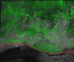
To obtain the water surface from the PIV images, an edge detection technique was applied because a strong light intensity gradient can be observed as a result of laser light reflection at the air–water interface (Reul, Branger & Giovanangeli Reference Reul, Branger and Giovanangeli2008; Shaikh & Siddiqui Reference Shaikh and Siddiqui2010). A Hilbert transform was then used to determine the phase of the overlying flow field (Melville Reference Melville1983; Buckley & Veron Reference Buckley and Veron2016; Porchetta et al. Reference Porchetta, Carlesi, Vetrano, van Beeck and Laboureur2022). An example of the PIV velocity field and the wave phase are shown in figure 2 to demonstrate the instantaneous flow field and the associated vortex structure downstream of the wave crest. Note that the coordinate system is defined as the x direction begins at the left edge of the FOV and the z direction points upwards from the mean free surface elevation.

Figure 2. (a) An example of instantaneous velocity field measured using the PIV technique at Uref = 10.0 m s−1. The horizontal velocities were subtracted by half of the reference velocity to illustrate vortex features. The red curve indicates the detected air–water interface. (b) Detected phase using Hilbert transform along the free surface.
2.3. Surface elevation measurements
An example of a time series of water surface elevation shows that the wave height, length and period increase as the wind speed increases (figure 3, table 1). The power spectrum of the 10-min wave data is shown in figure 4, which is used to determine the dominant wave frequency fp. The dominant wavelength λp and dominant wave speed cp (= λp fp) are then calculated based on linear wave theory. As expected, fp decreases with the increase of wind speed. A secondary, wind speed-dependent peak is observed in each spectral plot, which may be attributed to a nonlinear interaction among waves. This secondary peak appears to be twice the peak frequency which has been observed in other wind-wave systems (Hidy & Plate Reference Hidy and Plate1966; Lake & Yuen Reference Lake and Yuen1978; Komen Reference Komen1980). Table 1 summarizes important wave parameters, including the root-mean-square wave height Hrms and wave amplitude arms, the wave steepness kparms (kp = the dominant wave number), and the significant wave height Hs. Other flow related parameters and dimensionless parameters including bulk Reynolds number, roughness Reynolds number, wave Reynolds number and Bond number are also reported in table 1.

Figure 3. Examples of water surface elevations measured using the wave gauge for: (a) Uref = 6.0 m s−1; (b) Uref = 8.0 m s−1; (c) Uref = 10.0 m s−1.
Table 1. Summary of the parameters. Reference velocity Uref, 10 m equivalent velocity U 10, shear velocity of air  ${u_\ast }$, roughness length z 0, spectral peak frequency fp (obtained from wave power spectra shown in figure 2) and corresponding peak wavelength λp (calculated based on linear wave theory) and peak wave speed cp (= λp fp), root-mean-squared wave height Hrms, significant wave height Hs, peak wavenumber kp (= 2
 ${\rm \pi}$/λp), peak wave steepness kparms with arms being the wave amplitude, bulk Reynolds number
  $R{e_D} = {U_{ref}}D/{\nu _a}$ with D being the channel height and
  ${\nu _a}$ the kinematic viscosity of air, roughness Reynold number
  $R{e_0} = {u_\ast }{z_0}/{\nu _a}$ based on the shear velocity of air and roughness length, wave Reynolds number
  $R{e_w} = {c_p}{\lambda _p}/{\nu _w}$ based on wave properties with
  ${\nu _w}$ being the kinematic viscosity of water, and Bond number
  $Bo = ({\rho _w} - {\rho _a})g/(\sigma k_p^2)$ with
  ${\rho _w}$ being the water density,
  ${\rho _a}$ air density, g gravitational acceleration and
  $\sigma $ surface tension.


Figure 4. Power spectrum of water surface elevation determined from the wave gauge data.
2.4. Velocity triple-decomposition
The instantaneous velocity vector  $\boldsymbol{u}$ from the PIV measurements in the Cartesian coordinate system was decomposed into the phase-averaged velocity
  $\langle \boldsymbol{u}\rangle $ and turbulent fluctuating velocity
  $\boldsymbol{u^{\prime}}$, while the phase-averaged velocity can be further decomposed into the time-averaged velocity
  $\bar{\boldsymbol{u}}$ and the wave induced velocity
  $\tilde{\boldsymbol{u}}$ (Hsu et al. Reference Hsu, Hsu and Street1981), i.e.
 \begin{gather}\boldsymbol{u}(x,z,t) = \langle \boldsymbol{u}\rangle (x,z) + \boldsymbol{u^{\prime}}(x,z,t),\end{gather}
 \begin{gather}\langle \boldsymbol{u}\rangle (x,z) = \bar{\boldsymbol{u}}(z) + \tilde{\boldsymbol{u}}(x,z),\end{gather}
where u = (u, w) is the instantaneous velocity with u and w being the horizontal and vertical velocity components in the x and z directions, respectively. Since the two-dimensional PIV technique has been applied, no measurements on spanwise velocity v are available.
The phase-averaged and the time-averaged velocities were computed in the wave following coordinate system where  $\zeta = 0$ denotes the wavy water surface. The wave-induced component was then converted back onto the Cartesian coordinate system to determine the turbulent velocities. Therefore, the wave-induced and turbulent velocity components are resolved as a function of phase in the Cartesian coordinate system in the presence of waves. Figure 5 shows an example of velocity triple-decomposition into the time-averaged, wave-induced and turbulent velocity components at Uref = 6.0 m s−1. In the horizontal direction (figure 5a), we observe a classic boundary layer profile of the mean flow, an organized, phase dependent wave-induced velocity field and a turbulent flow field which also show a somewhat organized pattern close to the water surface. In the vertical direction (figure 5b), there seems to be a mean downward flow within the measurement location, with decreasing velocity towards the water surface but changing the direction within the wave height. Again, the wave-induced velocity is highly phase dependent and the turbulent fluctuations are relatively chaotic.

Figure 5. An example of velocity triple decomposition at Uref = 6.0 m s−1. (a) Horizontal velocity fields: instantaneous u, time averaged mean  $\bar{u}$, wave induced mean
  $\tilde{u}$ and turbulent velocity
  $u^{\prime}$. (b) Vertical velocity fields: instantaneous w, time averaged mean
  $\bar{w}$, wave induced mean
  $\tilde{w}$ and turbulent velocity
  $w^{\prime}$. Note that the wind blows from left to right and there is variation present on the contour colour bars from panel to panel.
2.5. Estimation of turbulent dissipation rate
To obtain the spatial distribution of turbulent dissipation rate,  $\varepsilon $, a ‘direct method’ can be applied for PIV measurements (Luznik et al. Reference Luznik, Zhu, Gurka, Katz, Smith and Osborn2007; Wang & Liao Reference Wang and Liao2016). The technique is based on the resolved velocity gradient from the PIV data, the continuity equation and necessary assumptions of local isotropy in small scales. The directly estimated turbulent dissipation rate reads:
 \begin{gather}
\varepsilon _D^A = 4\nu \left\langle {{{\left( {\frac{{\partial u^{\prime}}}{{\partial x}}} \right)}^2} + {{\left( {\frac{{\partial w^{\prime}}}{{\partial z}}} \right)}^2} + \frac{3}{4}{{\left( {\frac{{\partial u^{\prime}}}{{\partial z}}} \right)}^2} + \frac{3}{4}{{\left( {\frac{{\partial w^{\prime}}}{{\partial x}}} \right)}^2} + \left( {\frac{{\partial u^{\prime}}}{{\partial x}}\frac{{\partial w^{\prime}}}{{\partial z}}} \right) + \frac{3}{2}\left( {\frac{{\partial u^{\prime}}}{{\partial z}}\frac{{\partial w^{\prime}}}{{\partial x}}} \right)} \right\rangle .\end{gather}
\begin{gather}
\varepsilon _D^A = 4\nu \left\langle {{{\left( {\frac{{\partial u^{\prime}}}{{\partial x}}} \right)}^2} + {{\left( {\frac{{\partial w^{\prime}}}{{\partial z}}} \right)}^2} + \frac{3}{4}{{\left( {\frac{{\partial u^{\prime}}}{{\partial z}}} \right)}^2} + \frac{3}{4}{{\left( {\frac{{\partial w^{\prime}}}{{\partial x}}} \right)}^2} + \left( {\frac{{\partial u^{\prime}}}{{\partial x}}\frac{{\partial w^{\prime}}}{{\partial z}}} \right) + \frac{3}{2}\left( {\frac{{\partial u^{\prime}}}{{\partial z}}\frac{{\partial w^{\prime}}}{{\partial x}}} \right)} \right\rangle .\end{gather} From the two-dimensional PIV data, this method provides an instantaneous turbulent dissipation rate, which can be ensemble-averaged to obtain the phase-dependent  $\varepsilon $ for illustrating the wave effect. However, this method suffers from the coarse spatial resolution when the resolved spatial resolution is more than one order of magnitude larger than the Kolmogorov length scale (Saarenrinne & Piirto Reference Saarenrinne and Piirto2000; Luznik et al. Reference Luznik, Zhu, Gurka, Katz, Smith and Osborn2007; Xu & Chen Reference Xu and Chen2013). In contrast, the velocity spectrum remains quite robust even with coarse spatial resolution (Xu & Chen Reference Xu and Chen2013), such that
  $\varepsilon $ can be estimated reliably by fitting the spectrum to the universal Kolmogorov −5/3 law in the inertial subrange (Tennekes & Lumley Reference Tennekes and Lumley1972):
 \begin{equation}E(k) = \frac{{18}}{{55}}\beta {\varepsilon ^{2/3}}{k^{ - 5/3}},\end{equation}
where  $E(k)$ is the energy spectral density of the one-dimensional streamwise velocity determined in the main flow direction of the wavenumber domain, β = 1.6 is the universal Kolmogorov constant (Doron et al. Reference Doron, Bertuccioli, Katz and Osborn2001) and k is the wavenumber along the main flow direction.
In our time-resolved PIV measurements, the time-series data of instantaneous velocity at any given location above the height of wave crest can be used to calculate the energy spectral density in the frequency domain  $E(\,f)$, which can be converted to
  $E(k) = (U/2{\rm \pi} )E(\,f)$ by revoking the Taylor's frozen turbulence hypothesis, where the frequency
  $f = (U/2{\rm \pi} )k$ and U is the mean streamwise velocity (Li et al. Reference Li, Elliott, Call, Sansom, Jacobson and Wang2023).
Figure 6(a) presents one-dimensional streamwise velocity spectra at several z values in the wavenumber domain, obtained by converting from the frequency domain. At measurement locations within the range of 0.03–0.08 m where the length scale of turbulent eddies in the vertical direction is constrained by the water surface, we observed a clearly defined −5/3 slope in the range of 30–200 rad m−1, corresponding to eddy sizes of approximately 0.03–0.2 m. This suggests that a pronounced −5/3 slope can be observed in the range above the resolved largest length scale in the vertical direction. While turbulence eddies are typically isotropic in the inertial subrange, our findings indicate that the −5/3 slope in the streamwise velocity spectra deviates somewhat from the isotropic expectation, suggesting a degree of relaxation. However, we note that one-dimensional vertical velocity spectra are suppressed by the constraint in the resolved turbulent eddy sizes.

Figure 6. (a) One-dimensional velocity spectra in the horizontal wave number domain for the case of Uref = 10.0 m s−1 wind. The spectrum was converted from that in the frequency domain, which was computed from the time-series data. The shaded region indicates the inertial subrange where the −5/3 universal scaling law was applied to estimate turbulent dissipation rate. (b) Comparison of turbulence dissipation rate estimate using the spectrum and direct method above the maximum wave height for all three reference wind speeds. The dashed line is the linear fit.
After the inertial subrange was identified, regression can then be applied using (2.4) to estimate the turbulent dissipation rate. This method provides the time-averaged turbulent dissipation rate, denoted as  $\varepsilon _S^A$, above the wave crest over the entire measurement period and across all phases of wind waves. Fitting the velocity spectrum at different heights allows for the estimation of a vertical profile of turbulent dissipation rate. If the profile of
  $\varepsilon _S^A$ represents the unbiased estimate of turbulent dissipation rate, we can use this profile as a benchmark to correct underestimation caused by the coarse spatial resolution in the ‘direct method’ (Johnson & Cowen Reference Johnson and Cowen2018; Wu et al. Reference Wu, Wang, DiMarco and Tan2021).
We calculated the vertical profile of  $\varepsilon _D^A$ by averaging it on the same coordinate as that for
  $\varepsilon _S^A$. Therefore, the two vertical profiles can be directly compared, as shown in figure 6(b). The data indicate that
  $\varepsilon _D^A$ is smaller than
  $\varepsilon _S^A$ at almost all heights and underestimate the turbulent dissipation rates as expected. Using
  $\varepsilon _S^A = 0.9$, 1.9 and 4.2 m2 s−3 for an averaged value in the measurement region, the Kolmogorov length scales are estimated to be
  $\eta = {(\nu _a^3/\varepsilon )^{1/4}} = 0.25$, 0.20 and 0.17 mm, for Uref = 6.0, 8.0 and 10.0 m s−1, respectively. Hence, the ratio of PIV resolved spatial resolution to the Kolmogorov length
  $\varDelta /\eta $ is 8.1, 9.8 and 11.8, respectively. Saarenrinne & Piirto (Reference Saarenrinne and Piirto2000) showed the errors in dissipation rate falls more than 90 % when
  $10 < \varDelta /\eta < 15$, while Xu & Chen (Reference Xu and Chen2013) also estimated that dissipation rate using velocity gradients can be less than 25 % of the true dissipation rate when
  $\varDelta /\eta < 14$. The linear regression was used to find the relationship between the two methods:
  $\varepsilon _S^A = 3.9\varepsilon _D^A - 0.8$ (figure 6b). The factor of 3.9 agrees with the expected underestimation given the range of
  $\varDelta /\eta $ in this study (Saarenrinne & Piirto Reference Saarenrinne and Piirto2000; Xu & Chen Reference Xu and Chen2013).
Once the spatial distribution of instantaneous turbulent dissipation rate was estimated using the ‘direct method’, we follow the same procedure as in other mean flow and turbulent quantities to determine their phase-averaged values.
3. Classification of wind waves
3.1. Classification using dominant wavelength
Caulliez (Reference Caulliez2013) classified the wind waves into four categories, depending on the dissipation mechanism of surface waves: (1) capillary waves dissipated by molecular viscosity (category I); (2) gravity-capillary waves dissipated by generation of capillaries (category II); (3) gravity-capillary waves dissipated by generation of capillaries and microscale breaking (category III); and (4) short gravity waves dissipated by generation of micro- and macroscale breaking (category IV). Furthermore, Caulliez (Reference Caulliez2013) proposed a simple criterion based on dominant wavelength using the data from a wind-wave flume over the wind speed of 2.5–12 m s−1 and fetch of 2–26 m (table 2).
Table 2. Flow regime based on dominant wavelength λp proposed by Caulliez (Reference Caulliez2013), corresponding Bond number Bo and the shear-fetch based Reynolds number  $R{e_\ast }$ (
 $= {u_\ast }F/{\nu _a}$), based on the shear velocity of air and fetch length.

To demonstrate the wave classification and flow regime under these waves, we summarized our data along with available data of similar wind waves in laboratory scales, including those of Toba (Reference Toba1972), Siddiqui & Loewen (Reference Siddiqui and Loewen2007) and Caulliez (Reference Caulliez2013), in figure 7. Multiple groups of near-linear relationship are shown in the log–log plot of wavelength as a function of the shear velocity of air (figure 7a). Each group corresponds to a different fetch either within the same wave tank or across different studies. Not surprisingly, the data show that both wind shear and fetch correlate positively to the dominant wavelength. Regression of each data group results in an averaged slope of 0.98 in the log–log plot, suggesting a near-linear relationship between wavelength and the shear velocity.

Figure 7. (a) Comparison between dominant wavelength λp and the shear velocity of air  ${u_\ast }$ with data from Toba (Reference Toba1972), Siddiqui & Loewen (Reference Siddiqui and Loewen2007) and Caulliez (Reference Caulliez2013). The four flow regimes are marked based on the wavelength criterion (Caulliez Reference Caulliez2013, table 2). The slope of the dashed line is 0.98, which is the averaged slope over the different data groups. (b) Comparison between λp and
  $u_\ast ^{5/4}F$. The dashed fitted line is
  ${\lambda _p} = 0.082{(u_\ast ^{5/4}F)^{2/3}}$ with an R 2 value of 0.90.
To account for the combined effects of wind shear and fetch, we plot the dominant wavelength against the quantity  $u_\ast ^{5/4}F$ (figure 7b), an alternative of
  $U_\infty ^{5/4}F$ which is proposed by Lamont-Smith & Waseda (Reference Lamont-Smith and Waseda2008) to characterize the wave frequency
  ${f_p}\; \propto \; {(U_\infty ^{5/4}F)^{ - 0.43}}$, where U ∞ is the mean velocity measured 50 cm above the still water surface in their experiments. The shear velocity
  ${u_\ast }$ was obtained from log-law fitting to the mean velocity profile above the wind waves (see § 4.1). We found that using the quantity
  $u_\ast ^{5/4}F$ is an effective approach to combine wave and fetch in characterizing the dominant wavelength in various laboratory studies. The best-fit relationship across the range of laboratory wind and fetch data gives
  ${\lambda _p} = 0.082{(u_\ast ^{5/4}F)^{2/3}}$.
The data show that our wind wave conditions fall primarily within the category III (figure 7). The case of Uref = 6.0 m s−1 is near the boundary between categories II and III, and the case of Uref = 10.0 m s−1 is near the boundary of III and IV. This indicates the micro-scaling breakings started to form at Uref = 6.0 m s−1, but the surface was primarily covered by capillaries. For Uref = 10.0 m s−1, macroscale breaking was about to form on the water surface while the water surface was covered by microscale breaking. Direct visualization of water surface morphology (figure 8) supports the classification using the dominant wavelength. For Uref = 6.0 m s−1, water surface on the windward side of crest is mainly occupied by a smooth surface, while ripples are observed close to the crest and on the leeward side, known as parasitic capillaries which are commonly observed on short wind-wave surfaces (Cox Reference Cox1958; Zhang Reference Zhang1995). With increasing wind speed, surface roughness increases and the formation of parasitic capillaries is intensified. For Uref = 8.0 m s−1, a small portion of water surface may still be considered smooth. For Uref = 10.0 m s−1, the water surface is completely covered by capillaries and rollers, i.e. microscale breakers. Further increasing wind speed will lead to air-entraining breaking, which was visually confirmed. Similar observations were also made by Toba (Reference Toba1961) who reported that the lowest reference wind speeds for the occurrence of the air entrainment in wind waves were approximately 10.8 and 9.7 m s−1 at fetches of 5.5 and 7.0 m, respectively. Loewen & Siddiqui (Reference Loewen and Siddiqui2006) and Siddiqui & Loewen (Reference Siddiqui and Loewen2007) quantified that the breaking percentage increased from 11 % to 80 % as the wind speed increases from 4.5 to 7.4 m s−1 and increased to 90 % at 11 m s−1 by detecting micro-breaking waves at a fetch of 5.5 m.

Figure 8. Sample images of wind generated waves: (a) Uref = 6.0 m s−1; (b) Uref = 8.0 m s−1; (c) Uref = 10.0 m s−1. Note that the wind blows from left to right.
3.2. Dimensionless parameters
One shortcoming of the above wave classification is that all parameters are evaluated in the physical space, which hinders its application across different measurements. To explore using dimensionless parameters in classifying wind waves, the Bond number has been proposed instead of the dominant wavelength (Deike, Popinet & Melville Reference Deike, Popinet and Melville2015; Wu & Deike Reference Wu and Deike2021):  $Bo = ({\rho _w} - {\rho _a})g{L^2}/\sigma $, where
  ${\rho _w}$ is water density,
  ${\rho _a}$ is air density, g is gravitational acceleration, σ is surface tension and L is the characteristic length scale. In the present study, L is related to the wavelength through wavenumber
  ${k_p}$ as
  $L = 1/{k_p}$, where
  ${k_p} = 2{\rm \pi} /{\lambda _p}$. Because the only varying parameter in Bo is the wavelength in the air–water systems, the classification based on wavelength can be directly converted into a Bond number-based classification.
Here we seek to understand how Bond number can be scaled using dimensionless parameters that are related to wind and waves, so that wind waves can be directly classified using wind and wave parameters in the non-dimensional space. To incorporate shear velocity and fetch in the scaling, we test two dimensionless numbers: shear-fetch based Froude number  $F{r_\ast } = {u_\ast }/\sqrt {gF} $ and shear-fetch based Reynolds number
  $R{e_\ast } = {u_\ast }F/{\nu _a}$ (Wu Reference Wu1971, Reference Wu1973). The relationships of Bo versus
  $F{r_\ast }$ and Bo versus
  $R{e_\ast }$ are plotted in figure 9, including the data from Toba (Reference Toba1972), Siddiqui & Loewen (Reference Siddiqui and Loewen2007), Caulliez (Reference Caulliez2013) and Buckley & Veron (Reference Buckley and Veron2016). The plots in figure 9 are colour-coded using the wave age
  ${c_p}/{u_\ast }$ to illustrate the effect of wave age on the wave classification. Similar to figure 7(a), the data show groups of linear trends in Bo versus
  $F{r_\ast }$ on the log–log scale (figure 9a). The slopes of each line are averaged to be 1.91, giving
  $Bo \propto Fr_\ast ^{1.91}$. Examining all data, we found that wave age is not an influential factor in Bond number-based classification of wind waves as it appears uncorrelated with Bo. However, the relationship of Bo versus
  $R{e_\ast }$ shows that
  $R{e_\ast }$ can universalize the combined effect of wind shear and fetch across the range of available data and the regression suggests
  $Bo \propto Re_\ast ^{8/5}$ (figure 9b). Based on the classification thresholds using dominant wavelength proposed by Caulliez (Reference Caulliez2013), we estimated the thresholds of Bo and
  $R{e_\ast }$ to classify wind waves (table 2). The wind waves in categories I, II and IV are consistent with the wave shapes of nonlinear capillary waves, parasitic capillary waves, and spilling breakers for Bo = 1.47, 25 and 200, respectively, throughout numerical simulation (Wu & Deike Reference Wu and Deike2021). With the dimensionless parameterization, the proposed new classification can be easily applied to other studies, but it needs to be validated in the future.

Figure 9. Flow regimes in the space of dimensionless parameters. Data include the present study, and those from Toba (Reference Toba1972), Siddiqui & Loewen (Reference Siddiqui and Loewen2007), Caulliez (Reference Caulliez2013) and Buckley & Veron (Reference Buckley and Veron2016). (a) Shear-fetch based Froude number  $F{r_\ast }$ versus Bond number Bo. The dashed line indicates the averaged slope of 1.91 over the different data groups. (b) Shear-fetch based Reynolds number
  $R{e_\ast }$ versus Bond number Bo. The dashed fitting line is
  $Bo = 3.02 \times {10^{ - 7}}Re_\ast ^{8/5}$ with an R 2 value of 0.91. Note that the fill colour of each data point is coded with wave age cp/u ∗ according to the colour bar, while the symbol outline colour is coded as given in the legend at the top.
4. Velocity fields and stresses
4.1. Mean velocity
The horizontal velocity profiles averaged over the measurement duration and over all phases show a logarithmic shape similar to those in wall boundary flows (figure 10a). We consider the wave boundary as a quasi-stationary feature at the measurement location, so that the mean velocity profile averaged in the wave-following coordinate can be compared with that in wall bounded turbulent flows. To estimate the wind parameters, including shear velocity, 10 m equivalent velocity and roughness length over the water surface, we used the standard law-of-the-wall (LOW) fitting and selected data points for fitting based on a goodness-of-fit criterion, i.e. R 2 > 0.9. The results of the LOW fitting are summarized in table 1. The fitted shear velocities are positively correlated with the wind speed, and the data are consistent with those reported in the literatures for similar laboratory wind wave measurements, such as 6.9 m fetch by Toba (Reference Toba1972) and 5.5 m fetch by Siddiqui & Loewen (Reference Siddiqui and Loewen2007) (figure 10b).

Figure 10. (a) Profiles of mean horizontal velocity  $\bar{u}$ above the wave surface and the regression lines using law-of-the-wall equation; (b) shear velocity
  ${u_\ast }$ determined from the law-of-the-wall regression as a function of Uref. Data include those from Toba (Reference Toba1972) and Wu (Reference Wu1975) at a fetch of 6.9 and 11 m, respectively.
Based on the measured wind shear and wave parameters, the range of wave ages ( ${c_p}/{u_\ast } = 1.03\unicode{x2013} 1.10$) indicates that the wave fields in this study are young developing waves (Sullivan & McWilliams Reference Sullivan and McWilliams2010). Unlike previously reported numerical and experimental results that cover a wide range of wave ages (e.g. Rutgersson & Sullivan Reference Rutgersson and Sullivan2005; Yang & Shen Reference Yang and Shen2010; Buckley & Veron Reference Buckley and Veron2016), this study focuses on a narrow range of wave ages but various stages of wave categories (i.e. capillary, microscale and macroscale breaking).
4.2. Wave-induced velocity and stress
The phase-averaged wave-induced velocities ( $\tilde{u},\tilde{w}$) and wave-induced stress (analogues of Reynolds shear stress,
  $- \langle \tilde{u}\tilde{w}\rangle $) show consistent spatial patterns above the wind waves for different wind speeds (figure 11). In general,
  $\tilde{u}/{u_\ast }$ is positive over the crest and negative over the trough. Away from the surface (kpz > ∼0.5), the positive
  $\tilde{u}/{u_\ast }$ region on the crest changes its direction from positive to negative on the leeward side of the crest (x/λp = ∼0.25) and back to positive on the windward side of the crest (x/λp = ∼0.75). Close to the surface (kpz < ∼0.5), the direction rapidly shifts passing the crest on the leeward side of the crest (∼0.1 < x/λp < ∼0.25) and relatively smooth transition occurs on the windward side of the crest (∼0.7 < x/λp < ∼0.75). Also, while the intensified positive
  $\tilde{u}/{u_\ast }$ region is located near kpz = ∼0.5 on the crest, the intensified negative region moves close to the surface on the trough with increasing wind speed. The pattern of
  $\tilde{u}/{u_\ast }$ suggests that the wave perturbation causes the airflow to accelerate over the wave crest and decelerate over the wave trough. The patterns are generally consistent with the available experimental results reported with wave age of 1.4 and 2.5 at a fetch of 22.7 m (Buckley & Veron Reference Buckley and Veron2019). In addition, the data show that the positive
  $\tilde{u}/{u_\ast }$ region on the leeward side extends towards the near surface region of the trough and the magnitude decreases with increasing wind speed.

Figure 11. Phase-averaged normalized wave-induced velocities and wave-induced stress, i.e.  $\tilde{u}/{u_\ast }$,
  $\tilde{w}/{u_\ast }$ and
  $- \langle \tilde{u}\tilde{w}\rangle /u_\ast ^2$ at: (a) Uref = 6.0 m s−1; (b) Uref = 8.0 m s−1; (c) Uref = 10.0 m s−1. Note that the wind blows from left to right and there is variation present on the contour colour bars from panel to panel.
Here,  $\tilde{w}/{u_\ast }$ shows negative values on the leeward side and positive values on the windward side, a classic wave-induced velocity pattern above a wavy surface. Similar to
  $\tilde{u}/{u_\ast }$, the magnitude decreases with increasing wind speed, and the patterns are also consistent with a wave age of 1.4 and 2.5 (Buckley & Veron Reference Buckley and Veron2019). Examining the velocity in both horizontal and vertical directions, the wave effect can be interpreted as that the air flow accelerates above the crest with a downward velocity on the leeward side. The flow then moves upwards on the windward side and decelerates above the trough.
The pattern of  $- \langle \tilde{u}\tilde{w}\rangle /u_\ast ^2$ can be explained by the shear flow relative to the mean flow induced by the wave perturbation as indicated above. In the main flow field away from the water surface,
  $- \langle \tilde{u}\tilde{w}\rangle /u_\ast ^2$ is positive near crest on the leeward side and near trough on the windward side, while is negative near trough on the leeward side and near crest on the windward side. Similar to
  $\tilde{u}/{u_\ast }$, near the surface, the positive
  $- \langle \tilde{u}\tilde{w}\rangle /u_\ast ^2$ region on the leeward side extends towards the near surface region of the trough. The positive
  $- \langle \tilde{u}\tilde{w}\rangle /u_\ast ^2$ region, near the surface on the windward side, extends towards the near surface region of the crest.
Figure 12 shows the vertical profile of wave-induced velocities and stress over the course of one wavelength. The wave-induced velocities are negligibly small and wave-induced stress is confined within kpζ < ∼1.5, where ζ is the vertical coordinate in a wave-following system after phase-averaging, i.e. ζ = 0 is the water surface. Away from the confined region, the wave-induced accelerating and decelerating stages of flow compensate for each other, resulting in a quasi-steady flow. The vertical profile of wave-induced stress seems to be quite sensitive to the changing wind speeds and wave stages, compared with the profiles of  $\bar{\tilde{u}}/{u_\ast }$ and
  $\bar{\tilde{w}}/{u_\ast }$ in different cases. For the case of Uref = 6.0 m s−1, a negative peak appears near the water surface. A similar profile was also observed by Yang & Shen (Reference Yang and Shen2010) with the wave age of 2 (figure 12c). The magnitude of wave-induced stress decreases with increasing wind speed. Very different profiles of wave-induced stress were also observed by Yang & Shen (Reference Yang and Shen2010) with the wave age of 14 and 25 and by Buckley & Veron (Reference Buckley and Veron2016) with wave ages of 3.7–31.7. They presented large positive values near the surface and very small negative values above, indicating that the wave-induced stress is influenced by the wave ages. However, as our wave ages are quite similar, we suspect that the wave surface morphology may also contribute to the variability of the wave-induced stress profiles, in addition to the wave age.

Figure 12. Vertical profiles of normalized: (a) horizontal wave-induced velocities  $\bar{\tilde{u}}/{u_\ast }$; (b) vertical wave-induced velocities
  $\bar{\tilde{w}}/{u_\ast }$; and (c) wave-induced stresses
  $- \overline {\tilde{u}\tilde{w}} /u_\ast ^2$.
4.3. Turbulent intensity and Reynolds shear stress
The spatial distribution of the phase-averaged turbulent intensities (i.e. square-root of Reynolds normal stresses) and Reynolds shear stress demonstrates the phase-independent velocity fluctuations and the associated momentum flux above the wavy water surface (figure 13). The data show that the variations of turbulent intensities over different phases of waves are quite small. The values of turbulent intensities are of the same order of the shear velocity, with the horizontal turbulent intensity approximately twice that of the vertical turbulent intensity.

Figure 13. Phase-averaged normalized turbulent intensities and Reynolds shear stress, i.e.  $\sqrt {\langle {{u^{\prime}}^2}\rangle } /{u_\ast }$,
  $\sqrt {\langle {{w^{\prime}}^2}\rangle } /{u_\ast }$ and
  $- \langle u^{\prime}w^{\prime}\rangle /u_\ast ^2$ at: (a) Uref = 6.0 m s−1; (b) Uref = 8.0 m s−1; (c) Uref = 10.0 m s−1. Note that the wind blows from left to right.
Most of the flow field is covered by positive Reynolds shear stress (figure 13). Near the water surface, Reynolds shear stress decreases to close to zero. On the windward side immediately above the water surface, there appears a narrow region of negative Reynolds shear stress, which is likely attributed to the ‘blocking’ effect of the wavy water surface that moves slower than the air. Buckley & Veron (Reference Buckley and Veron2019) also reported negative values over a narrow region on the windward side of the crest (∼0.7 < x/λp < ∼0.9). In addition, they observed intensified positive Reynolds shear stress over a wide region on the leeward side (∼0.1 < x/λp < ∼0.4). In our data, the intensified positive Reynolds shear stress on the leeward side appears as more obvious in the case of Uref = 10.0 m s−1. The intensified Reynolds shear stress is one of the contributors to the strong shear production of TKE at this region (see figure 15). We note that the spatial pattern of the Reynolds shear stress in the wind-wave field is slightly different from that over a stationary wavy wall, where the maximum Reynolds shear stress is located on the trough (x/λp = ∼0.5) and approximately the height of wavy surface, while the negative values lie on both windward and leeward sides (e.g. Hudson, Dykhno & Hanratty Reference Hudson, Dykhno and Hanratty1996; Yang & Shen Reference Yang and Shen2010). The reason for the different spatial patterns between a stationary wavy wall and wind waves must result from the moving boundary, which leads to different slip boundary conditions.
The turbulent intensities and Reynolds shear stress over all phases show quite uniform vertical profiles for kpζ > ∼0.5 when averaged in the wave-following system (figure 14). Here,  $\sqrt {\overline {{{u^{\prime}}^2}} } /{u_\ast }$ increases slightly around the value of 2 with increasing wind speed, whereas
  $\sqrt {\overline {{{w^{\prime}}^2}} } /{u_\ast }$ remains close to 1. Additionally,
  $- \overline {u^{\prime}w^{\prime}} /u_\ast ^2$ seems to change its shape of profile at different wind speeds. For the case of Uref = 6.0 m s−1,
  $- \overline {u^{\prime}w^{\prime}} /u_\ast ^2$ is almost constant with a value of ∼0.7 at kpζ > ∼0.5. With increasing wind speed,
  $- \overline {u^{\prime}w^{\prime}} /u_\ast ^2$ increases near the water surface at kpζ < ∼1.2, but decreases away from the water surface at kpζ > ∼1.2. The changing shape of Reynolds shear stress may be due to the changing roughness and the boundary layer thickness with increasing wind speed. The changing shape of Reynolds shear stress profile was also observed by Buckley & Veron (Reference Buckley and Veron2019), who reported that the Reynolds shear stress increases with higher wind speed and lower wave age, while the thickness of the boundary layer gets thinner.

Figure 14. Vertical profiles of (a) horizontal turbulent intensities  $\sqrt {\overline {{{u^{\prime}}^2}} } /{u_\ast }$, (b) vertical turbulent intensities
  $\sqrt {\overline {{{w^{\prime}}^2}} } /{u_\ast }$, (c) Reynolds shear stresses
  $- \overline {u^{\prime}w^{\prime}} /u_\ast ^2$. All are normalized using shear velocity.

Figure 15. Phase-averaged shear production terms normalized by  $100u_\ast ^3/{\lambda _p}$ at: (a) Uref = 6.0
  ${\rm m}\ {\rm s}^{-1}$; (b) Uref = 8.0 m s−1; (c) Uref = 10.0 m s−1. Note that the wind blows from left to right and there is variation present on the contour colour bars from panel to panel.
Comparing the wave-induced and turbulent components (figures 12 and 14), we found that the magnitudes of  $- \overline {\tilde{u}\tilde{w}} /u_\ast ^2$ are approximately one-quarter of those of
  $- \overline {u^{\prime}w^{\prime}} /u_\ast ^2$ for the case of Uref = 6.0 m s−1, and the magnitude difference between
  $- \overline {\tilde{u}\tilde{w}} /u_\ast ^2$ and
  $- \overline {u^{\prime}w^{\prime}} /u_\ast ^2$ increases with increasing wind speed. This indicates a decreasing wave effect to air flow and the flow becomes more turbulent with increasing wind speed. The small wave-induced stresses compared with turbulent shear stresses are consistent with the results in the case of U 10 = 2.19 m s−1 (
 ${c_p}/{u_\ast } = 6.5$) at a fetch of 22.7 m observed by Buckley & Veron (Reference Buckley and Veron2019). We note that this case of Buckley & Veron (Reference Buckley and Veron2019) is the only one that falls within the same wind-wave category III as those in our study, i.e. microscale breaking waves (figure 9). For the cases in different wind-wave categories, i.e. wave age of 2.5 and 1.4, similar magnitudes of wave-induced stresses and Reynolds stresses were found (Buckley & Veron Reference Buckley and Veron2019). These results suggest that wind-wave categories and stages can significantly affect the mechanism of wave influence on the turbulence and wave-induced flow above the water surface.
5. Turbulent kinetic energy budgets
The governing equation of the TKE budget for the air flow over wind waves under a steady-state condition can be written as (Reynolds & Hussain Reference Reynolds and Hussain1972; Calhoun & Street Reference Calhoun and Street2001)
 \begin{equation}\varepsilon = \mathcal{P} + \mathcal{A} + {\mathcal{T}^t} + {\mathcal{T}^p} + {\mathcal{D}^\nu },\end{equation}
where  $\mathcal{P}$ is the shear production;
  $\varepsilon $ is the dissipation rate of TKE;
  $\mathcal{A}$ is the advection;
  ${\mathcal{T}^t}$ is the turbulence transport;
  ${\mathcal{T}^p}$ is the pressure transport and
  ${\mathcal{D}^\nu }$ is the viscous diffusion.
5.1. Production term
The production of TKE in the phase-averaged spatial domain consists of four terms (Calhoun & Street Reference Calhoun and Street2001; Yang & Shen Reference Yang and Shen2010; Buckley & Veron Reference Buckley and Veron2019):
 \begin{gather}\mathcal{P} = {\mathcal{P}_1} + {\mathcal{P}_2} + {\mathcal{P}_3} + {\mathcal{P}_4},\end{gather}
 \begin{gather}{\mathcal{P}_1} ={-} \langle u^{\prime}w^{\prime}\rangle \frac{{\partial \langle u\rangle }}{{\partial z}},\quad {\mathcal{P}_2} ={-} \langle {u^{\prime 2}}\rangle \frac{{\partial \langle u\rangle }}{{\partial x}},\quad {\mathcal{P}_3} ={-} \langle {w^{\prime 2}}\rangle \frac{{\partial \langle w\rangle }}{{\partial z}},\quad {\mathcal{P}_4} ={-} \langle u^{\prime}w^{\prime}\rangle \frac{{\partial \langle w\rangle }}{{\partial x}}.\end{gather}
To illustrate the contribution of each term to the production of TKE, the phase-averaged  ${\mathcal{P}_\textrm{1}}$,
  ${\mathcal{P}_\textrm{2}}$,
  ${\mathcal{P}_\textrm{3}}$ and
  ${\mathcal{P}_\textrm{4}}$ normalized by
  $100u_\ast ^3/{\lambda _p}$, following Calhoun & Street (Reference Calhoun and Street2001) and Yang & Shen (Reference Yang and Shen2010), are plotted in figure 15. Among the four terms, the shear production term
  ${\mathcal{P}_\textrm{1}}$ is the dominant term, which is generally one order of magnitude larger than
  ${\mathcal{P}_\textrm{2}}$ and
  ${\mathcal{P}_\textrm{3}}$, and two orders of magnitude larger than
  ${\mathcal{P}_\textrm{4}}$. Positive
  ${\mathcal{P}_\textrm{1}}$ is primarily concentrated on the leeward side, indicating that the majority of TKE production occurred in that region. A relatively small region of negative
  ${\mathcal{P}_\textrm{1}}$ is located near the water surface on the windward side. The negative shear production coincides with the negative Reynolds shear stress (figure 13), which may be attributed to the deceleration at that location when the wave travelling velocity is lower than the air flow for growing young waves. Here,
  ${\mathcal{P}_\textrm{2}}$ and
  ${\mathcal{P}_\textrm{3}}$ have similar patterns and show opposite signs in the spatial distribution. For instance, near the leeward side water surface,
  ${\mathcal{P}_\textrm{2}}$ is negative and
  ${\mathcal{P}_\textrm{3}}$ is positive, while
  ${\mathcal{P}_\textrm{2}}$ is positive but
  ${\mathcal{P}_\textrm{3}}$ is negative away from the surface. Although
  ${\mathcal{P}_\textrm{2}}$ and
  ${\mathcal{P}_\textrm{3}}$ are generally smaller than
  ${\mathcal{P}_\textrm{1}}$, accurate estimate of TKE production should include these terms. Especially close to the wavy surface, these two terms are not negligible. This is because the mean flow patterns are significantly altered near the wavy surface, which contributes to the production of turbulence that are associated with large gradients of velocities in addition to
  $\partial \langle u\rangle /\partial z$. Here,
  ${\mathcal{P}_\textrm{4}}$ is positive above the trough and negative above the crest. These general patterns of production terms are also similar to those over a stationary wavy surface (Calhoun & Street Reference Calhoun and Street2001) and wind generated waves with a longer fetch (Buckley & Veron Reference Buckley and Veron2019).
The relative importance of each component in the TKE production varies with wave ages. Within our narrow wave age range (1.03–1.10),  ${\mathcal{P}_\textrm{1}}$ is the single dominant term. Yang & Shen (Reference Yang and Shen2010) reported that
  ${\mathcal{P}_\textrm{1}}$ is dominant with the wave age of 2, 14 and 25. Yang & Shen (Reference Yang and Shen2010) also noted that
  ${\mathcal{P}_\textrm{3}}$ and
  ${\mathcal{P}_\textrm{4}}$ are one order of magnitude smaller, different from what we observed:
  ${\mathcal{P}_\textrm{4}}$ is one order of magnitude smaller than
  ${\mathcal{P}_\textrm{3}}$ and
  ${\mathcal{P}_\textrm{2}}$, and two orders of magnitude smaller than
  ${\mathcal{P}_\textrm{1}}$. However, both Yang & Shen (Reference Yang and Shen2010) and our observation suggest the dominant role of
  ${\mathcal{P}_\textrm{1}}$ in turbulence production in slow, young waves as that in the solid wavy boundary layer. Buckley & Veron (Reference Buckley and Veron2019) observed that
  ${\mathcal{P}_\textrm{1}}$ and
  ${\mathcal{P}_\textrm{2}}$ are one order of magnitude larger than
  ${\mathcal{P}_\textrm{3}}$ and
  ${\mathcal{P}_\textrm{4}}$ with wave age of 1.4, 2.5 and 6.5, equivalent to the wind speed of 16.63, 9.41 and 2.19 m s−1, respectively. Their observation also shows that
  ${\mathcal{P}_\textrm{2}}$ was similar to
  ${\mathcal{P}_\textrm{1}}$, and gradually took over and became larger than
  ${\mathcal{P}_\textrm{1}}$ in their case with the highest wind speed and the youngest wave. This is different from our observation and the numerical simulation of Yang & Shen (Reference Yang and Shen2010). We note that the experiment of Buckley & Veron (Reference Buckley and Veron2019) was conducted at a 22.7 m fetch, and their young waves are within the gravity wave regime where wave energy is primarily dissipated by micro- and macroscale breaking waves (figure 9). Air entrainment has likely occurred, which may have also altered the mechanism of turbulence production. In our observation, TKE production has a consistent mechanism across the wave category III: the Reynold shear stress works against the mean flow gradient, which transfers kinetic energy from the mean flow to the turbulence field.
5.2. Advection term
The phase-averaged advection of TKE by mean flow is defined as follows:
 \begin{equation}\mathcal{A} = {\mathcal{A}_1} + {\mathcal{A}_2},\quad {\mathcal{A}_1} ={-} \langle w\rangle \frac{{\partial \langle q\rangle }}{{\partial z}}\quad \textrm{and}\quad {\mathcal{A}_2} ={-} \langle u\rangle \frac{{\partial \langle q\rangle }}{{\partial x}},\end{equation}
where q is the TKE, taking a value of  $(u^{\prime}u^{\prime} + v^{\prime}v^{\prime} + w^{\prime}w^{\prime})/2$ with
  $v^{\prime}v^{\prime} = (u^{\prime}u^{\prime} + w^{\prime}w^{\prime})/2$ (Yousefi et al. Reference Yousefi, Veron and Buckley2021). The data show similar magnitudes for the vertical advection
  ${\mathcal{A}_\textrm{1}}$ and the horizontal advection
  ${\mathcal{A}_\textrm{2}}\; $(figure 16). Intensified
  ${\mathcal{A}_\textrm{1}}$ is located mainly close to the water surface, with positive value on the leeward side and negative on the windward side. For the lowest wind, an intensified positive
  ${\mathcal{A}_\textrm{1}}$ zone appears above the windward side of the crest. Intensified but weaker
  ${\mathcal{A}_\textrm{2}}$ is observed close the water surface with an opposite sign of
  ${\mathcal{A}_\textrm{1}}$. With increasing speed, we found an additional but weaker positive
  ${\mathcal{A}_\textrm{1}}$ zone immediately past the wave crest. This region coincides with the location of the vortical structure past the crest or air separation shown in figure 2(a). The presence of air separation may produce substantial vertical advection near the separation. This observation is consistent with the experimental results in air flow over hills (Poggi et al. Reference Poggi, Katul, Finnigan and Belcher2008).

Figure 16. Phase-averaged advection terms normalized by  $100u_\ast ^3/{\lambda _p}$ at: (a) Uref = 6.0 m s−1; (b) Uref =8.0 m s−1; (c) Uref = 10.0 m s−1. Note that the wind blows from left to right and there is variation present on the contour colour bars from panel to panel.
Compared with the turbulence production, the advection term is quite small. In a solid wavy surface, Calhoun & Street (Reference Calhoun and Street2001) found that advection is negative on the leeward side and positive on the windward side at a short distance above the wavy boundary. They suggest that the mean flow carries TKE-rich fluid away from the peak turbulence production region on the leeward side, resulting in negative advection there. The TKE-rich fluid is advected toward the windward, upslope boundary, resulting in positive advection on the windward side. However, in our wind-wave boundary, such organized TKE advection was not observed. The negative advection seems to only appear on the leeward side above a positive zone of  ${\mathcal{A}_\textrm{1}}\; $for the case of Uref = 6.0 m s−1. For the other two cases, this negative advection zone is too weak to appear in the distribution plot. In addition,
  ${\mathcal{A}_\textrm{2}}$ seems to offset a substantial portion of
  ${\mathcal{A}_\textrm{1}}\; $so that the net advection is quite weak. The difference of advection pattern between our measurements and those for a solid wavy boundary may be attributed to the travelling of water surface.
5.3. Turbulent transport term
The phase-averaged turbulent transport of TKE is defined as follows:
 \begin{equation}{\mathcal{T}^t} = \mathcal{T}_1^t + \mathcal{T}_2^t,\quad \mathcal{T}_1^t ={-} \frac{{\partial \langle qw^{\prime}\rangle }}{{\partial z}}\quad \textrm{and}\quad \mathcal{T}_2^t ={-} \frac{{\partial \langle qu^{\prime}\rangle }}{{\partial x}}.\end{equation}
The data show that for all wind speeds,  $\mathcal{T}_\textrm{1}^\textrm{t}$ is a dominant term in the turbulent transport of TKE (figure 17), indicating the dominant role of turbulent eddies that carry and exchange TKE in the vertical direction. Here,
  $\mathcal{T}_\textrm{1}^\textrm{t}$ is positive in a narrow region immediately adjacent to the water surface on the windward side and negative above the positive region. The result suggests that the redistribution of TKE due to turbulent motions mainly occurred in these areas (kpz < ∼0.7). In a high wind condition (Uref = 10.0 m s−1), the positive region of
  $\mathcal{T}_\textrm{1}^\textrm{t}$ close to the wavy surface shrinks and the negative region extends towards the wave crest.

Figure 17. Phase-averaged turbulent transport terms normalized by  $100u_\ast ^3/{\lambda _p}$ at: (a) Uref = 6.0
  ${\rm m}\ {\rm s}^{-1}$; (b) Uref = 8.0 m s−1; (c) Uref = 10.0 m s−1. Note that the wind blows from left to right and there is variation present on the contour colour bars from panel to panel.
5.4. Dissipation term
A high turbulent dissipation rate occurred near the water surface and decreased away from the surface (figure 18). The leeward side generally has higher TKE dissipation than the windward side. The high dissipation rate at the leeward side coincides with the strong turbulence shear production in that region but closer to the crest. With increasing wind speed, both windward- and leeward-side dissipation become similar. Immediately above the trough, the dissipation rate is smaller due to the shelter effect of the wave slope. This sheltered region near the trough was also observed using LES with a wave age of 1.4 (Husain et al. Reference Husain, Hara, Buckley, Yousefi, Veron and Sullivan2019).

Figure 18. Phase-averaged turbulent dissipation  $\varepsilon $ normalized by
  $100u_\ast ^3/{\lambda _p}$ at: (a) Uref = 6.0
  ${\rm m}\ {\rm s}^{-1}$; (b) Uref = 8.0 m s−1; (c) Uref = 10.0 m s−1. Note that the wind blows from left to right and there is variation present on the contour colour bars from panel to panel.
To further investigate turbulence dissipation and compare with that in the solid wall boundary layer, figure 19 plots the averaged dissipation rate across the entire phases with the corresponding canonical LOW scaling,  ${\varepsilon _{LOW}} = u_\ast ^3/\kappa z$, where
  $\kappa $ is the von Kármán constant, taken as 0.41. The data show that the dissipation rate in the wind wave field has a similar decaying profile away from the boundary as that from solid walls, but the value of dissipation rate in the wind-wave field are approximately 60–78 % smaller than that estimated using the LOW scaling. We found the mean ratio
  $\overline {\varepsilon /{\varepsilon _{LOW}}} = 0.21$, 0.35 and 0.40 for the cases of Uref = 6.0, 8.0 and 10.0 m s−1, respectively.

Figure 19. Vertical profile of turbulence dissipation rate: wind waves above water versus the corresponding law of the wall (LOW) above a solid boundary at the maximum wave height.
5.5. Turbulent kinetic energy budget
Finally, the phase-averaged TKE budget is illustrated in figure 20, which plots all budget terms and the residual term. In general, the three cases have similar spatial patterns of TKE budget terms, with subtle differences. All strong TKE budget terms are concentrated close to the water surface, except for the advection, which is patched in the entire measured region with weak substantial accumulations close to the surface.

Figure 20. Phase-averaged shear production  $\mathcal{P}$, advection
  $\mathcal{A}$, turbulent transport
  ${\mathcal{T}^t}$, turbulent dissipation
  $\varepsilon $ and residual Res terms normalized by
  $100u_\ast ^3/{\lambda _p}$ at: (a) Uref = 6.0 m s−1; (b) Uref = 8.0 m s−1; (c) Uref =10.0 m s−1. Note that the wind blows from left to right and there is variation present on the contour colour bars from panel to panel.
To summarize, the mechanism of the TKE can be interpreted as follows: strong shear in the mean flow above the wave surface produces TKE close to the wave crest and extends downwind, leading to a high positive shear production region on the leeward side. Approaching the wave trough, shear production reduces substantially to zero and changes to negative values on the windward side near the surface. The spatial distribution of mean advection of TKE appears to be relatively weak with some intensification close to the surface. The relatively weak spatial distribution of TKE advection is due to the opposite effect of mean flow and TKE production. The mean velocity is small close to the water surface where most of the TKE is produced, whereas weaker TKE is produced in the high flow region away from the surface. The turbulent transport process redistributes the TKE through moving TKE-rich fluids to the low TKE region. Therefore, there is an accumulated negative turbulent transport region that coincides with the high TKE production region, which mainly moves the TKE towards the region close to the water surface, showing a thin layer of positive turbulent transport immediately above the water surface. Turbulent dissipation accumulated close to the surface primarily dissipates the TKE generated from the shear production, i.e. local equilibrium.
Taken together, we found that the residual term is substantial within one wave height and shows a distinct spatial distribution. Specifically, most residuals show the opposite sign of the production term for balancing the TKE budget. The viscous diffusion was calculated and found to be negligible in this study. Although the current calculation does not include the TKE transport caused by pressure, its contribution to the TKE budget is usually small (Yang & Shen Reference Yang and Shen2010). Therefore, we suspect that the residual term is unlikely the result of an unresolved pressure transport term.
The difference in several TKE budget terms between windward and leeward sides of wind waves motivates us to examine them by conditional averaging based on the directions relative to the wind (figure 21). Not surprisingly, most differences occur within approximately one wave height ( $\mathrm{\zeta } <\, {\sim} 2{a_{rms}}$) above the water surface, except for the advection term (especially for the case of Uref = 10.0 m s−1). Consistently with the spatial distribution plot, turbulence production is larger on the leeward side, with the maximal value approximately twice that on the windward side. The peak production occurs between 0.5 and 1.5 wave amplitudes. Advection is relatively small, but the profiles of advection are not strictly consistent among all three cases. The turbulent transport is quite consistent on both sides. The negative turbulent transport term around the location of peak turbulence production indicates the mechanism of the turbulent transport, i.e. redistributing TKE from a TKE-rich to TKE-weak region. There seems to be no difference in TKE dissipation rate on leeward and windward sides. Together, the TKE is largely balanced for the three cases. Within one wave height, the residual appears to be positive on the windward side and negative on the leeward side, indicating that the TKE budget is not locally balanced at various phases. The difference of residual on windward and leeward sides substantially increases with increasing wind speed.

Figure 21. Averaged vertical profiles of turbulent kinetic energy budgets with averaging over all phase, leeward and windward sides: shear production  $\bar{\mathcal{P}}$, advection
  $\bar{\mathcal{A}}$, turbulent transport
  $\overline {{\mathcal{T}^t}} $, turbulent dissipation
  $\bar{\varepsilon }$ and residual Res normalized by
  $100u_\ast ^3/{\lambda _p}$ at: (a) Uref = 6.0 m s−1; (b) Uref = 8.0 m s−1; (c) Uref = 10.0 m s−1.
5.6. Vertical profiles of averaged turbulent kinetic energy budgets
The profiles of TKE budget terms averaged over all wave phases are plotted in figure 22. As discussed above, turbulence production occurs significantly close to the surface, with the peak at approximately ζ = 0.5arms to ζ = 1.5arms. The advection is relatively small. Turbulent transport is a source immediately above the water surface and changes to a sink within kpζ = 0.1–0.2. The turbulent dissipation rate is the primary sink term. The data indicate that the TKE budget is generally closed among these terms with relatively small residual for the two low wind conditions. There is a noticeable negative residual within ζ < arms for the highest wind speed condition. The peak magnitude of the residual is approximately half of the peak shear production. While the measurement uncertainty in high-order turbulence terms very close to the water surface may be a contributor, the exact cause of the observed residual is subject to future explorations.

Figure 22. Averaged vertical profiles of turbulent kinetic energy budgets normalized by  $100u_\ast ^3/{\lambda _p}$ at: (a) Uref = 6.0 m s−1; (b) Uref = 8.0 m s−1; (c) Uref = 10.0 m s−1.
Although the TKE budgets seem balanced, the production-dissipation ratio  $\bar{\mathcal{P}}/\bar{\varepsilon }$ is 1.49, 1.48 and 2.18 at ζ = 1.6arms, 1.2arms and 0.6arms for the case of Uref = 6.0, 8.0 and 10.0 m s−1, respectively, based on the location where the production is at a peak. The results for the two lower wind cases are slightly smaller than the production-dissipation ratio of 1.6 from numerical simulation with a wave age of 2 (Yang & Shen Reference Yang and Shen2010). The ratios are much smaller than the production-dissipation ratio of 3 reported by Shaikh & Siddiqui (Reference Shaikh and Siddiqui2010) with a wave age of approximately 2. The difference may be due to the method used for calculating the dissipation rate. For instance, our calculation indicates that the ‘direct method’ based on coarse-resolution PIV measurements without calibration may substantially underestimate the turbulence dissipation rate. With our data, we found that the production-dissipation ratio for the case of Uref = 10.0 m s−1 is approximately 45 % higher than the other two cases. We note that this case lies on the boundary of wave regimes III–IV, where substantial increase of microscale breaking waves would occur (Siddiqui & Loewen, Reference Siddiqui and Loewen2007). Therefore, we suspect that the increase in the production-dissipation ratio may be attributed to the increased surface roughness due to the onset (or near onset) of macroscale breakers and the significant coverage of microscale breakers on the water surface (figure 8).
6. Conclusions
In this paper, we presented an experimental study using particle image velocimetry (PIV) to resolve the turbulence structure over the wind waves and to analyse the budget of turbulent kinetic energy (TKE) of the overlying airflow. The experiment was designed to focus on developing young waves (i.e.  ${c_p}/{u_\ast } = 1.03\unicode{x2013} 1.10$) with a short fetch (i.e. F = 6.2 m), which were travelling slower than the bulk air flow velocity (i.e. wind-driven sea).
Using measured wave characteristics and the data from the literature, we found a dimensionless power-law relationship between Bond number and Reynolds number based on shear velocity and fetch:  $Bo\sim Re_\ast ^{8/5}$, which can be used to classify the wave regime depending on the primary mechanism of the wave energy dissipation. Although all wind waves are young in this study, they represent the entire regime of the wave category III, where the wave energy is mainly dissipated by capillaries and microscale breakers. The case of Uref = 6.0 m s−1 is close to the wave category II, and hence represents the early stage of wave category III, i.e. the water surface was primarily covered by capillaries with onset of microscale breaking. The case of Uref = 10.0 m s−1 is close to the wave category IV, and hence represents the late stage of wave category III, where the water surface was primarily covered by microscale breakers with onset of macro-breaking.
Through velocity triple-decomposition, our analysis provided the structures of wave-induced flow and the phase-independent turbulent flow above the varying phases of the waves. Our result demonstrated that the turbulent intensities and the velocity fluctuation-induced stresses are at least four times larger than the wave-induced counterparts, indicating that weaker kinetic energy in the air flow is coherent with wave motions and stronger kinetic energy is associated with phase-independent turbulence. However, the turbulent intensities were suppressed close to the wave boundary, where the organized turbulent motions generated intensified turbulent Reynolds shear stress on the leeward side of the waves.
The structures of TKE budget terms illustrate the wave-related spatial distributions of production, advection, transport and dissipation of the TKE. In a young wave covered by microscale breakers, the shear production dominated the generation of TKE, where the contributions from the normal stresses were small. This TKE generation mechanism is similar to that for solid wavy boundaries, and differs from those for the old waves or young waves at strong wind and long fetches that might be covered by macroscale breakers. In addition, the leeward side turbulence production was approximately twice of that on the windward side. The advection was weak compared with the TKE production. The turbulent transport term acted as expected, transporting the TKE away from the high turbulence production region.
Time-resolved PIV allowed us to estimate the dissipation rate of TKE above the wavy surface using the spectral fitting method to calibrate the directly calculated values from velocity gradients. Using an adequate sampling frequency, we resolved the universal Kolmogorov scaling in the inertial subrange of the energy cascade, which was used to estimate the turbulent dissipation rate that was not biased by the coarse spatial resolution in the PIV measurement. The data show that the intensified turbulent dissipation rate occurred at the wave crest, which coincided with the strong shear production in that region. The region immediately above the wave trough was sheltered by the leeward wave slope and showed weaker turbulence dissipation. The turbulent dissipation rates above the wind waves in our study were approximately 60–78 % smaller than those following the canonical law-of-the-wall (LOW) scaling.
Finally, the TKE budget analysis showed that the turbulence production, advection, turbulent transport and dissipation were generally in balance in all three cases. Although the TKE budgets seem balanced, the production-dissipation ratio for the highest wind speed was increased by 45 % compared with that for the two lower wind speeds. The increase of production-dissipation ratio might be caused by the increased roughness over the significant coverage of micro-breaking waves and near onset of macro-breakers. Further studies are needed to clarify this phenomenon.
Declaration of interests
The authors report no conflict of interest.


 Open access