


1. Introduction
The use of wind-tunnel testing with simplified geometries is a common method for investigating the fundamental aerodynamics of road vehicles. One widely used standard model is the Ahmed body, developed by Ahmed, Ramm & Faltin (Reference Ahmed, Ramm and Faltin1984), which is designed for vehicle geometries that generate large regions of separated flow. This model features a flat front face that is perpendicular to the flow, with rounded corners that connect to a long rectangular body. While the rear face of the Ahmed body can have various slant angles to mimic different types of vehicles, a flat-back Ahmed body with a rear face perpendicular to the flow has become popular for investigating bluff body aerodynamics. Other simple models with different frontal geometries and aspect ratios also produce large, separated flows with similar flow features. Examples of such models include the Windsor body (Howell, Sheppard & Blakemore Reference Howell, Sheppard and Blakemore2003), the ground transportation system (Croll et al. Reference Croll, Gutierrez, Hassan, Suazo and Riggins1996) and the simplified lorry model (Cabitza Reference Cabitza2013).
The measurements of Ahmed et al. (Reference Ahmed, Ramm and Faltin1984) for a flat-back Ahmed body at a Reynolds number of  $R{e_H} = 1.3 \times {10^6}$ show that the low-pressure zone at the rear face forms approximately 72 % of the total drag force. Here, ReH is defined as U∞H/ν, where U∞ is the free-stream velocity, H is the height of the rear face and ν is kinematic viscosity. In a more recent investigation at a lower ReH of 4 × 10⁵, Evrard et al. (Reference Evrard, Cadot, Herbert, Ricot, Vigneron and Délery2016) estimated that approximately 52 % of total drag is due to the low pressure at the rear face. Despite the apparent discrepancy between these two investigations, both highlight the importance of the flow motions that generate the low-pressure zone and increase the vehicle drag. Experimental and numerical investigations have identified several flow motions in the wake region, including bi-stable wake motions (Grandemange, Gohlke & Cadot Reference Grandemange, Gohlke and Cadot2012), vortex shedding (Khalighi, Chen & Iaccarino Reference Khalighi, Chen and Iaccarino2012; Grandemange, Gohlke & Cadot Reference Grandemange, Gohlke and Cadot2013) and bubble pumping (Duell & George Reference Duell and George1999; Volpe, Devinant & Kourta Reference Volpe, Devinant and Kourta2015). The bi-stable and vortex-shedding motions have been confirmed by many investigations while there are still discrepancies regarding the bubble-pumping motion.
The experiments of Grandemange et al. (Reference Grandemange, Gohlke and Cadot2012) demonstrated a pitchfork bifurcation in which the Ahmed body wake transitioned from a steady symmetric state into a steady asymmetric topology at ReH = 340. In the asymmetric state, the recirculation zone leaned towards an arbitrary spanwise side and maintained its orientation for an indefinite time. Grandemange et al. (Reference Grandemange, Gohlke and Cadot2012) showed that this asymmetry persists even in the turbulent regime at  $R{e_H} = 9.2 \times {10^4}$ although it occasionally switches from one spanwise side to another. The subsequent experiments showed that the switching in the turbulent regime is random, and the two asymmetric states are equiprobable (Grandemange et al. Reference Grandemange, Gohlke and Cadot2013; Volpe et al. Reference Volpe, Devinant and Kourta2015). Grandemange et al. (Reference Grandemange, Gohlke and Cadot2013) also estimated that the average switching period is approximately 1000H/U∞, three orders of magnitude greater than the vortex-shedding time scale. The bi-stable motion has been identified using several parameters, for example, based on the barycentre location of the wake deficit (Grandemange et al. Reference Grandemange, Gohlke and Cadot2013; Volpe et al. Reference Volpe, Devinant and Kourta2015; Haffner et al. Reference Haffner, Borée, Spohn and Castelain2020), spanwise pressure gradient on the rear face (Evrard et al. Reference Evrard, Cadot, Herbert, Ricot, Vigneron and Délery2016; Li et al. Reference Li, Barros, Borée, Cadot, Noack and Cordier2016; Dalla Longa, Evstafyeva & Morgans Reference Dalla Longa, Evstafyeva and Morgans2019) and the leading mode obtained from the proper orthogonal decomposition (POD) of velocity field or base pressure (Volpe et al. Reference Volpe, Devinant and Kourta2015; Pavia, Passmore & Sardu Reference Pavia, Passmore and Sardu2018; Fan et al. Reference Fan, Chao, Chu, Yang and Cadot2020; Pavia et al. Reference Pavia, Passmore, Varney and Hodgson2020).
The previous experimental and numerical investigations have led to a better understanding of the wake topology during asymmetric states. Using particle image velocimetry (PIV) measurements, Evrard et al. (Reference Evrard, Cadot, Herbert, Ricot, Vigneron and Délery2016) speculated that the mean topology of each bi-stable state consists of a large horseshoe vortex – the bound section of the horseshoe vortex crosses through the off-centred recirculation zone of the wake while the two trailing sections extend in the downstream direction. However, Perry, Pavia & Passmore (Reference Perry, Pavia and Passmore2016b) proposed the presence of an additional smaller horseshoe vortex to explain a small recirculating region seen on the opposing spanwise side. Using PIV measurement in cross-flow planes, Pavia et al. (Reference Pavia, Passmore and Sardu2018) suggested that the two horseshoe vortices are connected and form a single vortex with a relatively complex topology. Fan et al. (Reference Fan, Chao, Chu, Yang and Cadot2020) also proposed a similar vortex model. In a recent investigation, Pavia et al. (Reference Pavia, Passmore, Varney and Hodgson2020) developed a reduced-order model of the wake topology by applying POD to three-dimensional (3-D) flow measurements obtained using tomographic PIV (tomo-PIV). They identified two C-shaped horseshoe vortices on each spanwise side of the wake, and showed that the vortex crossing through the larger recirculation zone was stronger. However, the vortex topologies described by Evrard et al. (Reference Evrard, Cadot, Herbert, Ricot, Vigneron and Délery2016), Perry et al. (Reference Perry, Pavia and Passmore2016b), and Pavia et al. (Reference Pavia, Passmore and Sardu2018, Reference Pavia, Passmore, Varney and Hodgson2020) appear different from the toroidal vortex shown by the numerical simulations of Lucas et al. (Reference Lucas, Cadot, Herbert, Parpais and Délery2017) and Dalla Longa et al. (Reference Dalla Longa, Evstafyeva and Morgans2019). The instantaneous visualization of the latter investigations demonstrates a toroidal topology that is skewed to conform to the asymmetric state of the recirculation zone. The discrepancy warrants additional investigations of the wake topology during the bi-stable states.
Early evidence of periodic oscillations in the Ahmed body wake is seen in the hot-wire measurements of Duell & George (Reference Duell and George1999). The detailed measurements of Grandemange et al. (Reference Grandemange, Gohlke and Cadot2013) identified two flow oscillations in spanwise and vertical directions at Strouhal numbers of StH = 0.127 and 0.174. Here, StH is defined as f × H/U∞ where f is frequency. As expected, the vertical shedding was mainly present in the upper and lower shear layers, while the spanwise shedding was detected in the side shear layers. Volpe et al. (Reference Volpe, Devinant and Kourta2015) and Fan et al. (Reference Fan, Chao, Chu, Yang and Cadot2020) also measured similar StH values in their experiments. Plumejeau et al. (Reference Plumejeau, Delprat, Keirsbulck, Lippert and Abassi2019) observed greater StH when the Ahmed body was installed at a smaller ground clearance, but the values decreased to those reported by other investigations with increased ground clearance. The smaller time scale of the vortex-shedding motion relative to the bi-stability time scale indicates that several vertical and spanwise oscillations occur within the duration of each asymmetric state. Grandemange et al. (Reference Grandemange, Gohlke and Cadot2013) discussed that the bi-stability does not affect the dynamics of vertical shedding, but it results in a one-sided spanwise shedding from the stronger vertical shear layer. This one-sided vortex shedding is consistent with large hairpin vortices shed from the skewed side of the toroidal vortex seen in the numerical investigation of Dalla Longa et al. (Reference Dalla Longa, Evstafyeva and Morgans2019). However, the streamwise orientation of these hairpin vortices is opposite to the horseshoe/hairpin vortices described by Evrard et al. (Reference Evrard, Cadot, Herbert, Ricot, Vigneron and Délery2016), Perry et al. (Reference Perry, Pavia and Passmore2016b) and Pavia et al. (Reference Pavia, Passmore and Sardu2018, Reference Pavia, Passmore, Varney and Hodgson2020). To the authors’ knowledge, it is unclear how the later vortical structures interact with the vortex-shedding mechanism.
The bubble-pumping motion was originally defined to describe streamwise expansions and contractions of the separation bubble behind axisymmetric geometries such as disks and spheres (Berger, Scholz & Schumm Reference Berger, Scholz and Schumm1990). For axisymmetric geometries, this pumping motion occurs at low frequencies and features in-phase pressure fluctuations around the rear face of the body. For Ahmed body, Duell & George (Reference Duell and George1999) observed in-phase pressure fluctuations at StH of 0.07 only at the two spanwise sides of the rear face. In contrast, Volpe et al. (Reference Volpe, Devinant and Kourta2015) and Pavia et al. (Reference Pavia, Passmore and Sardu2018) observed in-phase pressure fluctuations at the top and bottom of the rear face at a similar StH of 0.08. These investigations attributed the in-phase pressure fluctuations to bubble-pumping motions limited to different planes of the wake. Another evidence of bubble pumping is seen in the spectra of area-averaged base pressure at StH = 0.04 to 0.08 (Khalighi et al. Reference Khalighi, Zhang, Koromilas, Balkanyi, Bernal, Iaccarino and Moin2001; Dalla Longa et al. Reference Dalla Longa, Evstafyeva and Morgans2019; Haffner et al. Reference Haffner, Borée, Spohn and Castelain2020). Haffner et al. (Reference Haffner, Borée, Spohn and Castelain2020) investigated the bubble pumping using cross-sectional area and strength of separation bubble from planar PIV measurements. The spectra of these quantities showed a peak at StH = 0.06, indicating energetic expansion and contraction of the separation bubble at a low frequency. In addition, evidence of bubble pumping has also been presented based on the spatial pattern of POD modes that capture in-phase fluctuations (Volpe et al. Reference Volpe, Devinant and Kourta2015). The POD analysis of the velocity field by Fan et al. (Reference Fan, Chao, Chu, Yang and Cadot2020) shows spatial modes that exhibit the pulsation of wake deficit and recirculation bubble in horizontal and vertical planes of the wake, respectively. Despite these observations, the detailed experimental investigation of Grandemange et al. (Reference Grandemange, Gohlke and Cadot2013) did not detect any indication of bubble pumping. In summary, the presence of the bubble-pumping mode and its 3-D dynamics remain unclear.
Understanding the complete 3-D dynamics of the Ahmed body wake is a challenging task, partly due to the limitations imposed by experimental and numerical simulations. In experiments, complex 3-D motions of the turbulent flow have to be inferred from point-wise hot-wire or 2-D-PIV measurements. To address this shortcoming, Perry et al. (Reference Perry, Almond, Passmore and Littlewood2016a) used tomo-PIV for 3-D wake measurements of a Windsor model. Their flow analysis was preliminary, but they highlighted the challenges regarding the number density of tracer particles and spatial-dynamic range for large-scale tomo-PIV measurements. Later, Pavia et al. (Reference Pavia, Passmore, Varney and Hodgson2020) utilized a large-scale tomo-PIV for an in-depth analysis of flow topology. Booysen, Das & Ghaemi (Reference Booysen, Das and Ghaemi2022) also used 3-D particle tracking velocimetry (3-D-PTV) to investigate Ahmed body wake at various side-slip angles. Although Pavia et al. (Reference Pavia, Passmore, Varney and Hodgson2020) and Booysen et al. (Reference Booysen, Das and Ghaemi2022) obtained 3-D measurements, hardware limitations did not allow for time-resolved analysis. As a result, their 3-D investigation was limited to ensemble averages and POD analysis, which hinders the full analysis of the flow dynamics.
The POD technique used by most previous investigations of the wake flow behind the Ahmed body and similar bluff bodies is based on the space-only formulation (e.g. POD analysis of Volpe et al. Reference Volpe, Devinant and Kourta2015; Perry et al. Reference Perry, Almond, Passmore and Littlewood2016a,Reference Perry, Pavia and Passmoreb; Pavia et al. Reference Pavia, Passmore and Sardu2018, Reference Pavia, Passmore, Varney and Hodgson2020; Fan et al. Reference Fan, Chao, Chu, Yang and Cadot2020; Podvin et al. Reference Podvin, Pellerin, Fraigneau, Evrard and Cadot2020; Booysen et al. Reference Booysen, Das and Ghaemi2022). In this technique, eigenvectors and eigenvalues of the two-point ‘spatial’ correlation tensor result in spatial modes that are modulated in time by a set of coefficients. The space-only formulation does not require time-dependent measurements, and the coefficients of the spatial modes have random time dependence (Sirovich Reference Sirovich1987; Schmid Reference Schmid2010; Towne, Schmidt & Colonius Reference Towne, Schmidt and Colonius2018). As a result, the spatial modes do not necessarily represent structures that are coherent in time and each mode may represent a mix of several flow motions with different frequencies. Such a decomposition of the velocity field is not ideal for identifying complex turbulent motions. In contrast to the space-only POD, the alternative space–time formulation decomposes the two-point ‘space–time’ correlation tensor into modes that each oscillate at a certain frequency (Lumley Reference Lumley1970; Picard & Delville Reference Picard and Delville2000). This technique is referred to as spectral POD (SPOD) and requires time-dependent flow realizations. To the authors’ knowledge, only Haffner et al. (Reference Haffner, Borée, Spohn and Castelain2020) and Venning et al. (Reference Venning, Mcqueen, Jacono, Burton, Thompson and Sheridan2022) applied SPOD to time-resolved planar PIV measurements of Ahmed body wake. The SPOD analysis of Haffner et al. (Reference Haffner, Borée, Spohn and Castelain2020) demonstrated evidence of pumping, shedding and a localized high-frequency mode at StH ~ 1, while the SPOD analysis of Venning et al. (Reference Venning, Mcqueen, Jacono, Burton, Thompson and Sheridan2022) characterized oscillatory modes behind a slant back body when varying its aspect ratio. Although computational fluid dynamics provides time-resolved flow fields, computational resources have limited access to long data sequences suitable for SPOD. An alternative technique that can address the shortcoming of space-only POD is dynamic mode decomposition. Dynamic mode decomposition was applied by Evstafyeva, Morgans & Dalla Longa (Reference Evstafyeva, Morgans and Dalla Longa2017) in a streamwise–spanwise plane of Ahmed body wake at 310 < ReH < 435, and by Dalla Longa et al. (Reference Dalla Longa, Evstafyeva and Morgans2019) for a simplified lorry model at ReH = 20 000.
The present investigation employs a unique approach to investigate the turbulent motions occurring in the wake of the Ahmed body. This approach involves the utilization of time-resolved tomo-PIV to measure 3-D velocity fields. Subsequently, these velocity fields are subjected to modal decomposition using SPOD, which allows for the identification of spatial modes at specific frequencies. The results address the lingering questions regarding the 3-D topology of bi-stability, vortex shedding and shear layer instability. Additionally, the findings reveal the existence of swinging/flapping motions over a wide StH range, which encompass certain characteristics associated with the bubble-pumping mode. In § 2, a detailed description of the experimental set-ups and the implementation of SPOD are presented. Sections 3 and 4 analyse the mean flow field and the barycentre location of the wake deficit, respectively. To facilitate comparison with existing literature, a space-only POD analysis is conducted in § 5. In § 6, the characterization of the spatio-temporal dynamics of the coherent structures using SPOD is presented. Finally, § 7 summarizes the most important observations and conclusions from this investigation.
2. Experimental methodology
The flow facility and the model's size were selected to enable time-resolved tomo-PIV within a measurement volume covering the full near-wake region. For this reason, the experiments were carried out in a water flume to benefit from two factors. First, for a desired Reynolds number, the smaller kinematic viscosity of water requires a smaller model and, therefore, a smaller measurement volume relative to experiments carried out using air in wind tunnels. Second, the density of water allows utilizing of large tracers that scatter more light for tomo-PIV imaging. Consequently, the smaller measurement volume and the larger tracer particles allowed the recording of tomo-PIV images with sufficient signal-to-noise ratio for a volumetric measurement with dimensions of 78 × 45 × 66 mm3 (equivalent to 2.6H × 1.5H × 2.2H) in the streamwise (x), vertical (y) and spanwise (z) directions, respectively. In addition to tomo-PIV, planar PIV measurements were carried out for preliminary characterization of the flow upstream and downstream of the model. In the following sections, the flow facility, planner PIV, tomo-PIV and the implementation of the modal decomposition are described.
2.1. Flow facility
The test section of the water flume has a length, width and height of 5.0 m, 0.68 m and 0.50 m, respectively. Two centrifugal pumps operate in parallel to circulate the flow in the flume. The reservoir of the flume consists of guide vanes, a honeycomb structure, and two layers of mesh and is connected via a small contraction section to the downstream test section. To provide optical access, the bottom and side walls of the test section are made of glass. The free-stream speed was set to  ${U_\infty } = 0.396\ \textrm{m}\ {\textrm{s}^{ - 1}}$ during all the measurements.
An Ahmed body was mounted upside down on a flat plate as seen in figure 1(a). The flat plate had a total length of 700 mm and a width of 620 mm. It featured an optimized leading-edge (LE) profile and a tapered trailing edge (Hanson, Buckley & Lavoie Reference Hanson, Buckley and Lavoie2012). The Ahmed body was located along the spanwise centre of the test section, 195 mm above the bottom wall of the flume, and 126 mm below the free surface of the water flume. These distances minimized the interference of the wake flow with the boundary layer on the flume walls and the free-surface waves.

Figure 1. (a) Schematic of the experimental configuration showing the test section of the water flume, the flat plate and the Ahmed body. (b) An upside-down schematic of the flat plate, Ahmed body, the laser sheet and two cameras used for planar PIV. The coordinate system is shown in the enlarged view of the model with the origin, O, at the centre of the rear face. (c) An upside-down schematic of the tomo-PIV configuration showing the four high-speed cameras, the laser light (green) and the measurement volume  $V$ (red).
The LE of the Ahmed body was at a distance of l 1 = 259 mm downstream of the plate's LE. At this location, the Reynolds number, Re, of the boundary layer based on l 1 and U∞, is 1.0 × 10⁵, slightly smaller than the critical Reynolds number for natural laminar-to-turbulent transition. Preliminary planar PIV measurements without the Ahmed body showed that the shape factor at this location was 1.86, confirming a transitional state (Schlichting & Gersten Reference Schlichting and Gersten2016). Therefore, a tripping tape with a rectangular cross-section of 1 mm × 4.5 mm (wall-normal height × streamwise length) was installed at l 2 = 160 mm downstream of the plate LE. The location of the tape (l 2) and height (h) were selected to ensure the laminar-to-turbulent transition according to the criteria described by Braslow & Knox (Reference Braslow and Knox1958) and Schlichting & Gersten (Reference Schlichting and Gersten2016). In addition, PIV measurements showed a shape factor of 1.47 at l 1 (without the Ahmed body), indicating that the trip wire resulted in a turbulent boundary layer. When the Ahmed body was not installed, the boundary layer thickness (based on 99 % of U∞) at l 2 was δ 2 = 5.7 mm, and at l 1 was δ 1 = 8.6 mm. The distance between the tripping tape and the Ahmed body is 17.5δ 2, which allows sufficient flow development before the flow reaches the Ahmed body (Elsinga & Westerweel Reference Elsinga and Westerweel2012).
The Ahmed body featured a flat back (no taper at the rear face) and had a 1 : 9.6 scale with respect to the original model of Ahmed et al. (Reference Ahmed, Ramm and Faltin1984). The model was machined from acrylic using a computerized numerical control router. The front and rear faces were painted in black to reduce reflections of the laser light during the experiments. The total length L of the model was 109.0 mm, and the height H and width W of the rear face were 30.0 mm and 40.0 mm, respectively. The uncertainty in these dimensions is approximately ±0.03 mm, accounting for potential thermal expansion or contraction of the model. The Reynolds number, defined as ReH = U∞H/ν, is 10 000. This ReH matches the ReH of recent numerical simulations by Podvin et al. (Reference Podvin, Pellerin, Fraigneau, Evrard and Cadot2020, Reference Podvin, Pellerin, Fraigneau, Bonnavion and Cadot2021). Podvin et al. (Reference Podvin, Pellerin, Fraigneau, Evrard and Cadot2020) employed POD analysis on the flow field derived from their numerical simulation and noted a good agreement with the experimental findings reported by Evrard et al. (Reference Evrard, Cadot, Herbert, Ricot, Vigneron and Délery2016) at a higher  $R{e_H} = 4.0 \times {10^5}$. Consequently, based on the observations of Podvin et al. (Reference Podvin, Pellerin, Fraigneau, Evrard and Cadot2020), the flow structures characterized in the current investigation may hold relevance at higher ReH. The model was connected to the plate using four cylinders with a 3 mm diameter. The clearance between the model and plate, C, was set to 11.2 mm. The clearance-to-height ratio of the current set-up is C/H = 0.37, which is larger than the C/H = 0.17 used by Ahmed et al. (Reference Ahmed, Ramm and Faltin1984). The larger clearance is chosen to compensate for the large δ 1/H = 0.29 of the current experiment. In general, Grandemange et al. (Reference Grandemange, Gohlke and Cadot2013) and Cadot, Evrard & Pastur (Reference Cadot, Evrard and Pastur2015) showed that bi-stability is present when C/H > 0.1.
As shown from the enlarged view of the Ahmed body in figure 1(b), the origin of Cartesian coordinate system O is at the middle of the rear face. In the following sections, the directions of the axes are defined as x in the streamwise direction, y in the spanwise direction and z in the direction normal to the flat plate. The components of instantaneous velocity are defined as U, V and W, following the same order as the coordinate system axes. Lastly, the lowercase letters u, v and w represent the fluctuating velocity components. The mean value and the absolute magnitude of any quantity are indicated as  $\langle \cdots \rangle $ and
  $|\cdots |$, respectively.
2.2. Planar particle image velocimetry
A planar PIV experiment was carried out to characterize the mean flow upstream and downstream of the Ahmed body. The PIV system consisted of two Imager ProX (LaVision GmbH) 14-bit CCD cameras with a pixel size of 7.4 × 7.4 μm2. Both cameras were equipped with Nikon lenses with a focal length of f = 105 mm and an aperture setting of f/5.6. The upstream and downstream measurements were conducted simultaneously using a common laser sheet aligned with the x–y plane, as shown in figure 1(b). The first camera imaged the field-of-view (FOV) indicated as FOV1 upstream of the Ahmed body, while the second camera imaged FOV2 downstream of the model. Both cameras imaged the flow using cropped sensors with 2047 × 1001 pixel. FOV1 and FOV2 had similar dimensions of 146.4 × 71.5 mm2 and 149.8 × 73.2 mm2, respectively. The digital resolution of FOV1 was 71.5 μm pixel−1, and the digital resolution of FOV2 was 73.2 μm pixel−1. A dual-cavity Nd:YAG laser (Gemini, NewWave Research) with 110 mJ pulse−1 was used as the illumination source. Combining two cylindrical and two spherical lenses converted the laser beam into a wide sheet with 1 mm thickness covering FOV1 and FOV2. Two sets of 1500 double-frame images were collected at an acquisition rate of 9.4 Hz and with a laser pulse separation of Δt = 1500 μs.
Glass beads with the thin silver coating (SG02S40 Potters Industries) were used as tracer particles for planar PIV. These monodisperse tracers have a mean diameter of dp = 2 μm and a density of  ${\rho _p} = 4\ \textrm{g}\ \textrm{c}{\textrm{m}^{ - 3}}$ (Das & Ghaemi Reference Das and Ghaemi2021). Their response time,
  ${t_p} = {\rho _p}d_p^2/18\mu$, and settling velocity,
  ${u_p} = ({\rho _p} - \rho )d_p^2g/18\mu$, are 9.8 × 10⁻⁷ s and 7.2 × 10⁻⁶ m s−1, respectively. Here, ρ and μ are water's density and dynamic viscosity, and g is the gravitational acceleration. Assuming that the flow time scale is estimated based on the vortex-shedding period (~7 × H/U∞), the Stokes number of these tracers, Stk = tp/tf, is 1.8 × 10⁻⁶, which is smaller than the recommended value of 0.1 (Samimy & Lele Reference Samimy and Lele1991). The Froude number Fr is also estimated as up/U∞, which is 1.8 × 10⁻⁵, several orders of magnitude smaller than unity (Bewley, Sreenivasan & Lathrop Reference Bewley, Sreenivasan and Lathrop2008).
To improve the image's signal-to-noise ratio, the minimum intensity of all images was calculated and then subtracted from each image. The resulting images were then normalized using the average intensity of the images. The 2-D vector fields were obtained through double-frame cross-correlation with a multi-pass algorithm in Davis 8.3 (LaVision GmbH). The final interrogation window was 32 × 32 pixels (2.2 × 2.2 mm2). A window overlap of 75 % was applied between neighbouring interrogation windows, resulting in 55 and 73 vectors along the height and width of the model, respectively. Approximately 3 % of the velocity vectors were identified as spurious and were removed based on the universal outlier detection method (Westerweel & Scarano Reference Westerweel and Scarano2005).
2.3. Tomographic particle image velocimetry
The tomo-PIV system consisted of four high-speed cameras (Phantom v611, Vision Research) imaging the illuminated volume from the camera arrangement shown in figure 1(c). The cameras feature a complementary metal-oxide-semiconductor sensor with 1280 × 800 pixels; each pixel 20 × 20 μm2. The two upstream cameras had a small viewing angle of approximately 5° with respect to the z-axis, while the two downstream cameras had a larger viewing angle of approximately 35°. To minimize image distortion at high imaging angles, the latter two cameras imaged through two water-filled prisms installed on the glass wall of the flume. The cameras had a digital resolution of approximately 70 μm pixel−1 and a magnification of 0.3. All cameras had Nikon lenses ( f = 105 mm) and Scheimpflug adapters. An aperture setting of f/22 was used for all cameras, resulting in a depth-of-focus of approximately 66 mm.
A dual-cavity Nd:YLF laser (DM20-527DH, Photonics Industries) with 20 mJ pulse−1 illuminated the measurement volume. The laser light was directed perpendicular to the flat plate (in the negative y direction) from the bottom glass wall of the water flume. The beam passed through multiple cylindrical lenses to first form an elliptical cross-section. Then four knife edges at the bottom wall of the flume cropped the edges of the expanded beam. This resulted in a rectangular cross-section and a relatively ‘top hat’ intensity profile across its cross-section. The illuminated volume had a cross-section of (Δx, Δz) = (85 mm, 67 mm) at y = −H/2 and (81 mm × 65 mm) at y = +H/2 plane. The measurement volume, indicated by the red colour in figure 1(c), had dimensions of 78 × 45 × ~66 mm3 (2.6H × 1.5H × 2.2H) in x, y and z, respectively.
To address the limited energy of the high-repetition laser, we used relatively large polystyrene spheres (TS250 Dynoseeds) with a mean diameter of dp = 250 μm and density of 1.05 g cm−3. The larger tracers increase the intensity of the scattered light  $({\sim} d_p^2)$, while their nearly neutral density in water results in a small response time of
  ${t_p} = 4 \times {10^{ - 3}}\ \textrm{s}$. Based on the vortex-shedding time scale, the estimated Stk number of these particles is 7.6 × 10⁻³, which is smaller than the maximum recommended value of 0.1 (Samimy & Lele Reference Samimy and Lele1991). The settling velocity of the tracers is also 1.9 × 10⁻³ m s−1, and therefore their Fr is 4.7 × 10⁻³, which is also several orders of magnitude smaller than unity (Bewley et al. Reference Bewley, Sreenivasan and Lathrop2008). Based on visual inspection of the tomo-PIV images, the particle image diameter is between 3 and 5 pixels, and the seeding density is 0.03 particles per pixel. Combining these two parameters results in the maximum recommended source density of Ns = 0.3 (Scarano Reference Scarano2012).
The imaging system was calibrated using a dual-plane 3-D calibration plate (type 10, Lavision GmbH) that was traversed to five z locations with 12 mm spacing. The mapping function of measurement volume was initially constructed using a third-order polynomial fit in Davis 8.4 (LaVision GmbH). To improve the calibration accuracy, this was followed with a volume self-calibration procedure (Wieneke Reference Wieneke2008). Using self-calibration, the root-mean-square of the calibration error reduced from 1.3 to 0.05 pixels, which is below the recommended 0.1 pixels.
The tomo-PIV images were recorded as double-frame and time-resolved single-frame images. The double-frame images allowed for obtaining a longer duration of non-correlated data at a low acquisition frequency for faster statistical convergence. In contrast, the single-frame data at a higher acquisition frequency allowed for resolving the high-frequency dynamics of the flow. For double-frame recording, 3 datasets of 3107 double-frame images were collected at 25 Hz using a laser pulse separation of Δt = 3500 μs. The total duration of each set is 124.3 s, which is equivalent to 1641 × H/U∞ (larger than the bi-stability time scale of ~1000H/U∞). For time-resolved measurements, 10 datasets of 6212 single-frame images were collected at a recording rate of 280 Hz. Each time-resolved dataset was 22.2 s, which is 292 × H/U∞ (shorter than the bi-stability time scale). The time-resolved data can be used for spectral analysis of the flow between StH of 0.003 and 21.2 (half the acquisition frequency). A similar maximum particle displacement of around 18 pixels was obtained for both double-frame and single-frame images. The 10 time-resolved datasets provide the stochastic ensemble required for SPOD computations.
For processing the tomo-PIV images, first, the minimum of all images was subtracted from each image. This was followed by subtracting the local minimum of image intensity within a kernel size of 5 pixels. The images were also normalized using a local average with a kernel of 100 pixels. The measurement volume was reconstructed using the fast multiplicative algebraic reconstruction technique (fast-MART) in Davis 8.4 (LaVision GmbH) following the algorithm of Atkinson & Soria (Reference Atkinson and Soria2009). The reconstructed volume has 1116 × 645 × 931 voxels in x, y, and z directions. The vector field was obtained using the direct correlation in Davis 8.4 (LaVision GmbH). The final interrogation volume was 48 × 48 × 48 voxels (3.36 × 3.36 × 3.36 mm3) with a 75 % overlap, resulting in 93 × 54 × 78 vectors in the x, y and z directions, respectively. The spurious vectors formed approximately 2 % of the total number of vectors. These vectors were detected using the universal outlier detection (Westerweel & Scarano Reference Westerweel and Scarano2005) and replaced using linear interpolation. Finally, the measurement volume,  $V$, was further cropped to 83 × 47 × 56 vectors (2.3H × 1.3H × 1.6H) to remove noisy borders. The fast-MART and direct correlation processes for each single-frame dataset (6213 images) were carried out using a 16-core processor (AMD Ryzen 9 5950X) over a duration of 2 weeks.
The bi-stability motion, discussed earlier, leads to prolonged periods of spanwise asymmetry in the flow field. Consequently, achieving spanwise symmetry of time-averaged velocity fields becomes challenging, particularly for tomo-PIV measurements that generate large datasets and require intensive computations. To address this challenge, we adopt the technique utilized by Podvin et al. (Reference Podvin, Pellerin, Fraigneau, Evrard and Cadot2020) to enforce spanwise symmetry. This involves appending the original vector fields of the 10 time-resolved tomo-PIV datasets with 10 additional copies, each flipped along the spanwise direction. The copied vector fields also undergo a reversal of the spanwise velocity component to ensure a divergence-free flow field. A similar symmetrization process is also applied to the 3 double-frame tomo-PIV datasets. The resulting symmetry-enforced database eliminates any spanwise asymmetry in time-averaged fields and modal decomposition and improves the statistical convergence of the results.
2.4. Modal decomposition
The POD computations are carried out based on the snapshot method of Sirovich (Reference Sirovich1987) and using the 6 symmetry-enforced double-frame tomo-PIV datasets. The vector fields obtained from the double-frame images are temporally uncorrelated, resulting in faster statistical convergence of the POD modes. To begin the POD computations, three instantaneous velocity fluctuations (u, v and w) from all the grid points of each tomo-PIV snapshot were stacked into a column vector  ${\boldsymbol{x}_i} \in {R^N}$. Here, N equals the number of flow variables times the number of grid points (3 × 218 456). The xi vectors were then grouped together in a 2-D matrix
  ${\boldsymbol{\mathsf{X}}} = [{\boldsymbol{x}_1},{\boldsymbol{x}_2}, \ldots ,{\boldsymbol{x}_M}] \in {R^{N \times M}}$ where M = 18 642 is the total number of snapshots. The singular value decomposition of the correlation matrix, XT X, was computed to obtain UσVT. The parameters U and V are the left and right matrices of eigenvectors, and σ is the eigenvalues matrix. The matrix of spatial modes is
  $\boldsymbol{\varPhi}$ = XUσ−1/2, where each spatial POD mode,
  $\varPhi$j, is a column of
  $\boldsymbol{\varPhi}$. The energy of each POD mode, σj, is obtained from the diagonal components of σ. This method is equivalent to carrying out an eigendecomposition of XT X according to XT XU = Uσ−1/2 and calculating the spatial modes following
  $\boldsymbol{\varPhi}$ = XUσ−1/2.
An SPOD code was developed in MATLAB (MathWorks) based on the SPOD algorithm detailed by Towne et al. (Reference Towne, Schmidt and Colonius2018). The computations used the 20 symmetry-enforced time-resolved tomo-PIV datasets, each consisting of 6212 snapshots recorded at 280 Hz. Each dataset is divided into 3 equal segments with 50 % overlap, which results in a total of S = 60 segments. The data within each data segment are organized in a 2-D matrix,  ${{\boldsymbol{\mathsf{X}}}_k} = [{\boldsymbol{x}_1},{\boldsymbol{x}_2}, \ldots ,{\boldsymbol{x}_M}] \in {R^{N \times M}}$, where k is the segment's index varying from 1 to 60. Similar to POD, xi is a column-wise vector of the tomo-PIV snapshot with a length of N = 3 × 218 456. The total number of snapshots within each segment, M, equals 3106 since the segment length is half the size of the time-resolved dataset. The current segmentation procedure is slightly different from the algorithm described by Towne et al. (Reference Towne, Schmidt and Colonius2018), in which one long dataset was divided into multiple segments. This difference is imposed by the finite onboard memory of high-speed cameras, which prevents acquiring longer datasets.
In addition, due to the limited memory of the processing computers, each data segment, Xk, is processed separately. The rows of Xk matrices are multiplied by a Hamming window and then converted to the frequency domain by performing the fast Fourier transform operation. The Fourier representation of each Xk is  ${{\boldsymbol{\mathsf{Q}}}_k} = [{\boldsymbol{q}_1},{\boldsymbol{q}_2}, \ldots ,{\boldsymbol{q}_K}] \in {C^{N \times K}}$, where ql is a column-wise vector of Fourier coefficients at frequency index l, varying from 1 to M/2 = 1553. The index l = 1 corresponds to a frequency of 0 Hz, while the last index of l corresponds to 140 Hz (StH = 10.6). The resolution of the spectral domain is also 0.09 Hz (equivalent to ΔStH of 0.007). Next, the column vectors ql corresponding to frequency index l from all Qk matrices are grouped into a single matrix,
  ${{\boldsymbol{\mathsf{Q}}}_l^{\prime}} = [\boldsymbol{q}_l^1,\boldsymbol{q}_l^2, \ldots ,\boldsymbol{q}_l^S] \in {C^{N \times S}}$. Once
  ${{\boldsymbol{\mathsf{Q}}}_l^{\prime}}$ is computed, matrix Cl, for each frequency index l, is constructed as
  ${{\boldsymbol{\mathsf{C}}}_l} = (1/S){\boldsymbol{\mathsf{Q}}}^{\prime T}_l{{\boldsymbol{\mathsf{Q}}}_l^{\prime}}$ using the method of snapshots (Sirovich Reference Sirovich1987). Finally, the SPOD modes and eigenvalues are computed following
  ${{\boldsymbol{\mathsf{C}}}_l}{\boldsymbol{\phi }_l} = {\boldsymbol{\phi }_{\!l}}{\boldsymbol{\lambda }_l}$ and
  ${\boldsymbol{\varPsi }_{\!l}} = {{\boldsymbol{\mathsf{Q}}}_l}{\boldsymbol{\phi }_l}$. Here, ϕl is the eigenvector of Cl, and
  $\boldsymbol{\varPsi}\!$l includes the SPOD modes at frequency index l. The matrix
  $\boldsymbol{\varPsi}\!$l has the form of
  $[\varPsi _l^1,\varPsi _l^2, \ldots ,\varPsi _l^S] \in {C^{N \times S}}$. The eigenvalue
  $\lambda _l^n$ corresponding to SPOD mode n at wavenumber l is embedded in the diagonal elements of λl.
In the analysis of the subsequent sections, the SPOD modes are used to reconstruct a periodic reduced-order model (ROM) at selected frequencies (Nekkanti & Schmidt Reference Nekkanti and Schmidt2021). The ROM model of the U component at frequency index, l, is computed according to
 \begin{equation}{U_{ROM}} = \langle U\rangle /{U_\infty } + \mathcal{R}e({\varPsi _{u,l}}/{U_\infty } \times {\textrm{e}^{\textrm{i}\varPhi }}).\end{equation}
Here,  $\mathcal{R}e$ is the real part of a complex number. For any grid point of the measurement domain,
  $\langle U\rangle$ is the average velocity,
  $\varPsi_{u}$,l denotes the streamwise component of SPOD mode at frequency index l. The phase
  $\varPhi$ is also defined as 2
 ${\rm \pi}$flt in which fl is the frequency (in Hz) corresponding to index l. The duration of each ROM cycle is different as it is equal to 1/fl. Similar equations based on
  $\varPsi_{v}$,l and
  $\varPsi_{w}$,l are also used to reconstruct ROMs of the V and W components indicated as VROM and WROM, respectively. In addition, to reconstruct the ROM of the velocity fluctuations, (2.1) is reduced to
 \begin{equation}{u_{ROM}} = \mathcal{R}e({\varPsi _{u,l }}/{U_\infty } \times {\textrm{e}^{\textrm{i}\varPhi }}).\end{equation}
Similar equations are also used to reconstruct vROM and wROM.
3. Mean flow characterization
This section evaluates the mean flow characteristics using planar- and tomo-PIV measurements. Figure 2(a) shows the  $\langle U\rangle$/U∞ contour in the x–z plane upstream of the Ahmed body. A small reversed flow region is observed over the flat plate right after the tripping tape at x/H ≈ −7. The streamlines show a parallel flow that encounters the front face of the Ahmed body, forming a stagnation point on the front face of the body at z/H ~ 0. In figure 2(b), contours of
  $\langle U\rangle$/U∞ in the x–z plane show a recirculation zone downstream of the Ahmed body holding two counter-rotating vortices. The strongest backflow is between the two vortices and reaches a magnitude of ~0.25U∞, similar to the observations of the previous investigations (Grandemange et al. Reference Grandemange, Gohlke and Cadot2013; Volpe et al. Reference Volpe, Devinant and Kourta2015; Perry et al. Reference Perry, Almond, Passmore and Littlewood2016a; Fan et al. Reference Fan, Chao, Chu, Yang and Cadot2020; Pavia et al. Reference Pavia, Passmore, Varney and Hodgson2020).

Figure 2. Flow streamlines and contours of normalized streamwise velocity from planar PIV (a) upstream and (b) downstream of the Ahmed body in the y/H = 0 plane.
The clearance between the bottom face of the Ahmed body and the flat plate affects the underbody flow rate. If this flow rate is too small, a secondary separation bubble forms on the flat plate downstream of the Ahmed body, and the bi-stable switching of the wake disappears (Plumejeau et al. Reference Plumejeau, Delprat, Keirsbulck, Lippert and Abassi2019). In figure 2(b), no indication of a secondary separation bubble is present, suggesting the underbody clearance is sufficient. The sufficient underbody clearance is also evident when the shear layer thickness is compared with the underbody clearance. The shear layer thickness is 0.2C in the current investigation, estimated based on the region of intense vorticity. This value is comparable to the shear layer thickness of 0.1C estimated by Grandemange et al. (Reference Grandemange, Gohlke and Cadot2013) and 0.27C by Kang et al. (Reference Kang, Essel, Roussinova and Balachandar2021).
The length of the separation bubble, Ls, is an important parameter since it is inversely proportional to the base drag of the vehicle (Grandemange, Gohlke & Cadot Reference Grandemange, Gohlke and Cadot2014). This parameter can be estimated from the location of the saddle point labelled with the letter ‘S’ in figure 2(b). The estimated Ls of the current flow is 1.24H, which is smaller than Ls of 1.4H to1.5H reported at higher ReH by Grandemange et al. (Reference Grandemange, Gohlke and Cadot2013), Volpe et al. (Reference Volpe, Devinant and Kourta2015) and Fan et al. (Reference Fan, Chao, Chu, Yang and Cadot2020). The smaller Ls of the current investigation is consistent with the trend observed by Plumejeau et al. (Reference Plumejeau, Delprat, Keirsbulck, Lippert and Abassi2019), showing that the Ls reduced from 1.41H to 1.31H when ReH decreased from 4.29 × 10⁵ to 1.43 × 10⁵.
The state of the boundary layer developed on the upper surface of the Ahmed body can be evaluated by characterizing the intensity of the fluctuations. At the streamwise location of x/H = 0, the maximum standard deviation of the velocity fluctuations within the boundary layer is approximately 0.2U∞, indicating the turbulent state of the upper boundary layer. Similar measurements by Grandemange et al. (Reference Grandemange, Gohlke and Cadot2013) indicated a maximum standard deviation of 0.35U∞ at the upper edge of the rear face.
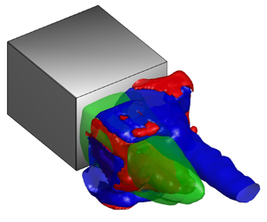
The 3-D topology of the mean flow is characterized using the symmetry-enforced double-frame tomo-PIV measurements in figure 3. The 3-D isosurface of zero streamwise velocity (green isosurface) in figure 3(a) shows the boundaries of the mean separation bubble. The main vortical structure of the mean flow is also a toroidal vortex, as seen from the purple isosurface of the Q-criterion (Hunt, Wray & Moin Reference Hunt, Wray and Moin1988). The 2-D streamlines of figure 3(d) in z/H = 0 plane show that the two mean recirculation regions are identical, and the saddle point is at y/H ~ 0.2, as expected from the averaging of the symmetry-enforced data.

Figure 3. The 3-D and 2-D visualizations of the mean velocity field from tomo-PIV measurements. (a) Isosurface of  $\langle U\rangle$/U∞ = 0 (green) and normalized Q-criterion,
  $Q{H^2}/U_\infty ^2 = 0.48$ (purple). (b) Isosurfaces of
  $\langle W\rangle$/U∞ = ±0.1, and (c)
  $\langle V\rangle$/U∞ = ±0.1. Red shows +0.1, and blue shows −0.1. (d) Two-dimensional contours of
  $\langle U\rangle$/U∞ at z/H = 0 plane, (e) contour of
  $\langle W\rangle$/U∞ at y/H = 0 and ( f) contour of
  $\langle V\rangle$/U∞ at z/H = 0.
In figure 3(b), the negative and positive isosurfaces of  $\langle W\rangle$/U∞ show different topologies for the isosurfaces of downward and upward flow. The downward flow (blue isosurface) consists of two lobes. The shape indicates that the intense downward motions are on either side of the spanwise centre at y/H ~ ±0.33. In contrast, the upward flow topology (red isosurface) shows a single triangular-shaped region with the peak of the upward at the spanwise centre. Kang et al. (Reference Kang, Essel, Roussinova and Balachandar2021) also demonstrated two off-centred downward zones and a strong central upward for an Ahmed body placed in a thick boundary layer. Despite the shape difference, the volume within the displayed isosurfaces of upward and downward is approximately similar. Figure 3(e) also shows the upward and downward motions where the streamlines curve around the end of the separation bubble at x/H ~ 1. In addition, the recirculation zones generate an upward zone close to the upper edge and a downward zone close to the lower edge of the rear face.
The spatial organization of the two opposing spanwise motions is shown in figures 3(c) and 3( f). There are small zones of spanwise motion near the rear face in figure 3(c), while the larger zones are farther downstream. The zones of spanwise motions are elongated in the z direction and symmetric with respect to the y/H = 0 plane. Figure 3( f) shows that the weaker spanwise motions form upstream of the recirculation zone, while the stronger motions form close to the end of the separation bubble at x/H ~ 1.
4. Barycentre of the wake deficit
To evaluate the presence of the bi-stable mode and investigate the oscillations of the separation bubble, the barycentre of the wake deficit is analysed. Unlike previous investigations that calculated the barycentre within 2-D planes (e.g. Grandemange et al. Reference Grandemange, Gohlke and Cadot2013; Haffner et al. Reference Haffner, Borée, Spohn and Castelain2020), the current study computes the barycentre using 3-D velocity fields obtained from tomo-PIV measurements. Using the 3-D data, the spanwise barycentre location is calculated following
 \begin{equation}{y_b} =
\frac{\displaystyle{\iiint_{\varOmega} {y(1 - U/{U_\infty
})\,\textrm{d}\varOmega} }}{\displaystyle{\iiint_{\varOmega} {(1 - U/{U_\infty
})\,\textrm{d}\varOmega} }}.\end{equation}
\begin{equation}{y_b} =
\frac{\displaystyle{\iiint_{\varOmega} {y(1 - U/{U_\infty
})\,\textrm{d}\varOmega} }}{\displaystyle{\iiint_{\varOmega} {(1 - U/{U_\infty
})\,\textrm{d}\varOmega} }}.\end{equation}
Here, the integrals are calculated within volume  $\varOmega$ of the wake where U/U∞ < 1. A similar equation is used for calculating xb and zb.
Figure 4 displays the distributions of the joint probability density function (JPDF) for yb and zb. These distributions were obtained from the original three double-frame datasets and ten time-resolved datasets of tomo-PIV measurements in figures 4(a) and 4(b), respectively. The symmetry-enforced data are not utilized in this figure to allow for the observation of asymmetry present in the original dataset. Figure 4(a) shows two high probability yb locations at ±0.05H due to the spanwise bi-stability (Grandemange et al. Reference Grandemange, Gohlke and Cadot2013). These yb/H locations are consistent with the values reported by Grandemange et al. (Reference Grandemange, Gohlke and Cadot2013) and Fan et al. (Reference Fan, Chao, Chu, Yang and Cadot2020). However, a slight disparity in the magnitudes of the two peaks is observed due to an insufficient statistical convergence resulting from the prolonged duration of each bi-stable state. As expected, the wake only demonstrates one high probability location in the z direction at zb/H = −0.03, indicating no bi-stable motion in the vertical direction. For time-resolved data with shorter overall duration, the asymmetry increases in figure 4(b) showing a stronger peak at yb = +0.05H relative to the peak at yb = −0.05H. Upon inspecting the time-series datasets, it is evident that out of the 10 datasets, yb maintained a positive value in 8 datasets, was negative in one dataset and switched between positive and negative in the remaining dataset. In terms of duration, yb was positive in 88 % of the measurement time, and negative in 12 % of the time for the time-resolved data. The asymmetry can be avoided by collecting additional datasets, but the prolonged tomo-PIV data processing prohibited us from collecting additional datasets. As explained in § 2.3, the asymmetry of the data is addressed by creating a symmetry-enforced dataset, achieved through appending the original dataset with a spanwise-flipped copy of the data.

Figure 4. The JPDF of the barycentre of momentum deficits for (a) 3 double-frame and (b) 10 time-resolved tomo-PIV datasets.
Figure 5(a) displays the pre-multiplied power spectral density (PSD) of normalized fluctuations of the barycentre locations (i.e.  ${x^{\prime}_b}/H$,
  ${y^{\prime}_b}/H$, and
  ${z^{\prime}_b}/H$). These spectra depict both the frequency and magnitude of fluctuations in the separation bubble's position. For calculating the PSD, the time series of barycentre location from each time-resolved tomo-PIV dataset is divided into 3 segments with 50 % overlap and then weighted by a hamming window. Therefore, in total 30 segments, each 73H/U∞ long, are used for calculating the PSDs. Note that the analysis of figure 5 is also carried out using the original data without symmetry enforcement since it does not affect the PSDs of figure 5.

Figure 5. (a) The pre-multiplied PSD of the normalized fluctuations in barycentre location  $({x^{\prime}_b}/H,{y^{\prime}_b}/H,{z^{\prime}_b}/H)$, (b) the normalized fluctuations in backflow volume,
  $\varPi '\!\big/$
 $\langle \varPi\rangle$. (c) The coherence function computed between
  $({x^{\prime}_b}/H,{y^{\prime}_b}/H,{z^{\prime}_b}/H)$ and
  $\varPi'\!\big/$
 $\langle \varPi\rangle$.
At the low StH end of the spectrum, the pre-multiplied PSD of  ${y^{\prime}_b}$ exhibits higher energy levels than that of
  ${x^{\prime}_b}$ and
  ${z^{\prime}_b}$, possibly due to spanwise bi-stability. The PSD shows two regions of high energy: the first is between StH values of 0.03 and 0.09, which is similar to the StH range reported previously for bubble-pumping motion (Duell & George Reference Duell and George1999; Khalighi et al. Reference Khalighi, Zhang, Koromilas, Balkanyi, Bernal, Iaccarino and Moin2001; Volpe et al. Reference Volpe, Devinant and Kourta2015; Dalla Longa et al. Reference Dalla Longa, Evstafyeva and Morgans2019). However, additional investigation is required to determine if the
  ${y^{\prime}_b}$ fluctuations at this range are due to the bubble-pumping motion. The pre-multiplied PSD of
  ${x^{\prime}_b}$ also displays low-frequency fluctuations between StH = 0.05 and 0.1, but they are less significant than those observed for
  ${z^{\prime}_b}$. The second region of high energy for
  ${y^{\prime}_b}$ is between StH values of 0.11 and 0.18 and is attributed to the barycentre oscillations generated by vortex-shedding motion, which is proposed based on its similarity to the StH value reported for spanwise vortex shedding (Grandemange et al. Reference Grandemange, Gohlke and Cadot2013). Similar energetic motions are also observed in the pre-multiplied PSD of
  ${x^{\prime}_b}$ and
  ${z^{\prime}_b}$, with narrower and stronger peaks. The peak of
  ${z^{\prime}_b}$ occurs at StH = 0.16, which is consistent with vertical vortex shedding observed by Grandemange et al. (Reference Grandemange, Gohlke and Cadot2013). Finally, a third small peak at StH of 1.15 is visible in the
  ${x^{\prime}_b}$ fluctuations spectrum.
Figure 5(b) presents the pre-multiplied PSD of the fluctuations in the separation bubble's volume. The volume of the separation bubble,  $\varPi$, is identified where the velocity U < 0, and its fluctuations are denoted as
  $\varPi$′. The spectrum exhibits a low StH zone at StH = 0.04 to 0.1, which is energetically more significant than the low StH zone observed for
  ${y^{\prime}_b}$ in figure 5(a). Haffner et al. (Reference Haffner, Borée, Spohn and Castelain2020) investigated the pre-multiplied PSD of the recirculation size based on the streamwise-spanwise cross-sectional area obtained from 2-D-PIV measurements. They found a narrow peak at StH = 0.06, which they attributed to the bubble-pumping mode. The narrower peak in Haffner et al. (Reference Haffner, Borée, Spohn and Castelain2020) could be due to the use of 2-D area instead of the 3-D volume used in figure 5(b). However, further investigation of the corresponding flow motions is necessary to confirm if the low StH range observed in figure 5(b) is consistent with the bubble-pumping motion. The mid-frequency peak at StH of 0.15 to 0.19 is in agreement with the vortex-shedding process, which varies the volume of the separation bubble through vortex roll-up. Additionally, the third peak at StH = 1.15 is more pronounced than the peak observed for
  ${x^{\prime}_b}$ in figure 5(a). This high StH motion with smaller energy is attributed to shear layer instabilities mentioned in studies by Duell & George (Reference Duell and George1999), Khalighi et al. (Reference Khalighi, Zhang, Koromilas, Balkanyi, Bernal, Iaccarino and Moin2001) and Haffner et al. (Reference Haffner, Borée, Spohn and Castelain2020).
To investigate the correlation between the fluctuations in barycentre location and the separation volume, the coherence function between each coordinate of the barycentre fluctuations  $({x^{\prime}_b},{y^{\prime}_b},{z^{\prime}_b})$ and
  $\varPi$′ is shown in figure 5(c). The analysis reveals that at the vortex shedding StH of 0.16, the fluctuations in
  $\varPi$′ correlated with the fluctuations of all three coordinate locations
  ${x^{\prime}_b}$,
  ${y^{\prime}_b}$ and
  ${z^{\prime}_b}$. Interestingly, the low StH fluctuations of
  $\varPi$′ correlate with the fluctuations in
  ${x^{\prime}_b}$, whereas it shows a smaller correlation with
  ${y^{\prime}_b}$ and
  ${z^{\prime}_b}$. At the higher StH of 1.15, the fluctuations in
  $\varPi$′ also only correlated with
  ${x^{\prime}_b}$.
The results indicate that the fluctuations of  $\varPi$′ at StH = 0.04 to 0.1 are a result of low energy oscillations of the barycentre in the x-direction, consistent with the expected dynamics of the bubble-pumping motion. However, the fluctuations of
  $\varPi$′ at the vortex shedding StH of 0.15 to 0.19 occur along with the barycentre oscillations in all three coordinate directions. Notably, the shear layer instabilities at StH = 1.15 only result in barycentre oscillations in the x-directions, leading to fluctuations of
  $\varPi$′. It's important to note that although the spectral analysis of figure 5 allows us to compare the StH of these motions with those reported in the literature, it only allows us to speculate about the mechanism behind them. In § 6, we will demonstrate the dynamics of these motions at each StH in detail using the SPOD technique.
5. Proper orthogonal decomposition
Several studies have used the POD technique to model and characterize the wake dynamics of an Ahmed body. For instance, Volpe et al. (Reference Volpe, Devinant and Kourta2015) and Pavia et al. (Reference Pavia, Passmore and Sardu2018) employed POD to analyse pressure fluctuations at the rear-face. Pavia et al. (Reference Pavia, Passmore and Sardu2018) also performed POD of stereoscopic PIV measurements at two cross-flow planes. Perry et al. (Reference Perry, Almond, Passmore and Littlewood2016a), Pavia et al. (Reference Pavia, Passmore, Varney and Hodgson2020) and Booysen et al. (Reference Booysen, Das and Ghaemi2022) applied POD analysis to 3-D flow measurements. Fan et al. (Reference Fan, Chao, Chu, Yang and Cadot2020) compared the POD analysis of planar PIV measurements with the POD of planar data from a numerical simulation. Podvin et al. (Reference Podvin, Pellerin, Fraigneau, Evrard and Cadot2020, Reference Podvin, Pellerin, Fraigneau, Bonnavion and Cadot2021) applied POD to a large 3-D domain obtained from direct numerical simulations. To identify similarities and highlight limitations of the POD analysis, the present study briefly compares its results with those of previous investigations.
Figure 6(a) shows the energy distribution of the ten leading POD modes. The first mode in the current study contains 9.9 % of the total turbulent kinetic energy, which is smaller than the energy reported in previous studies using 3-D measurements. For example, the first mode contained 15 % of the turbulent kinetic energy in Perry et al. (Reference Perry, Almond, Passmore and Littlewood2016a), 21 % in Pavia et al. (Reference Pavia, Passmore, Varney and Hodgson2020) and 33 % in Booysen et al. (Reference Booysen, Das and Ghaemi2022). This discrepancy is likely due to several factors, including the lower ReH of the current experiment and differences in the duration, domain size and spatial resolution of the measurements. Nevertheless, the energy of the first mode in the current experiment is close to the 8 % energy reported for the lead mode by Podvin et al. (Reference Podvin, Pellerin, Fraigneau, Evrard and Cadot2020) at a similar Reynolds number of ReH = 10 000. Figure 6(b) shows that the remaining POD modes have significantly smaller energy relative to the first mode. Specifically, the second mode contains approximately 1.4 % of the total energy, and the higher-order modes contain an even smaller percentage of the total energy. The large energy difference between the first POD mode and the remaining modes is consistent with previous POD investigations.

Figure 6. (a) Energy of 10 leading POD modes. Panels (b) to (g) show the spatial structures of the u-component for the six leading POD modes ordered from modes 1 to 6, respectively. The red and blue iso-surfaces show similar magnitudes of the streamwise component but with opposite signs.
The u-component of the first POD mode in figure 6(b) exhibits two streamwise-elongated structures with opposite signs, resulting in a strong antisymmetry of the wake with respect to the vertical midspan plane of y = 0. This mode is known as the spanwise symmetry-breaking mode (Pavia et al. Reference Pavia, Passmore and Sardu2018). Similar modes have been observed in 3-D POD analyses by Pavia et al. (Reference Pavia, Passmore, Varney and Hodgson2020), Podvin et al. (Reference Podvin, Pellerin, Fraigneau, Evrard and Cadot2020), and Booysen et al. (Reference Booysen, Das and Ghaemi2022). A spanwise antisymmetry has also been observed in the first POD mode of base pressure in Volpe et al. (Reference Volpe, Devinant and Kourta2015) and cross-flow PIV fields in Pavia et al. (Reference Pavia, Passmore and Sardu2018). While Pavia et al. (Reference Pavia, Passmore, Varney and Hodgson2020) and Podvin et al. (Reference Podvin, Pellerin, Fraigneau, Evrard and Cadot2020) attributed the first POD mode to the bi-stability motion, other investigations, including Volpe et al. (Reference Volpe, Devinant and Kourta2015), Pavia et al. (Reference Pavia, Passmore and Sardu2018), and Booysen et al. (Reference Booysen, Das and Ghaemi2022), associated the first POD mode with both bi-stability and spanwise vortex shedding, based on spectral analyses of the mode coefficient.
The second POD mode in figure 6(c) consists of two large structures at the upper and lower halves of the wake. The two structures are antisymmetric with respect to the horizontal mid-height plane (z = 0). The vertical antisymmetry of this mode resembles the 3-D structures shown in mode 3 of Pavia et al. (Reference Pavia, Passmore, Varney and Hodgson2020). The third mode in figure 6(d) shows two pairs of structures at x/H ~ 1 and 2 that are also antisymmetric with respect to the horizontal mid-height plane (z = 0) and demonstrates a strong streamwise periodicity. Similar modes with vertical antisymmetry and streamwise periodicity are seen in Fan et al. (Reference Fan, Chao, Chu, Yang and Cadot2020) and Podvin et al. (Reference Podvin, Pellerin, Fraigneau, Evrard and Cadot2020). These features are consistent with the spatial characteristics of a vertical vortex-shedding process. Examining the coefficients of modes 2 and 3 made it apparent that these two modes undergo oscillations with a consistent phase shift of  ${\rm \pi}$/2, which results in periodic oscillations in the streamwise direction.
Figure 6(e) displays the fourth POD mode, which exhibits three large streamwise-elongated structures. Two structures with similar signs are observed at the spanwise sides, while a structure with the opposite sign is located along the mid-span of the wake. This mode exhibits both spanwise and vertical symmetry, as it is symmetric with respect to both the vertical mid-span plane and the horizontal mid-height plane. Previous studies have reported similar symmetry-preserving modes in the POD analysis of base pressure (Volpe et al. Reference Volpe, Devinant and Kourta2015; Pavia et al. Reference Pavia, Passmore and Sardu2018), planar PIV (Pavia et al. Reference Pavia, Passmore and Sardu2018; Fan et al. Reference Fan, Chao, Chu, Yang and Cadot2020), tomo-PIV (Pavia et al. Reference Pavia, Passmore, Varney and Hodgson2020), and 3-D-PTV measurements (Booysen et al. Reference Booysen, Das and Ghaemi2022). Modulating this spatial pattern results in the elongation and shortening of the separation bubble in the streamwise direction, which can be associated with the bubble-pumping motion.
In figure 6( f), the fifth POD mode exhibits streamwise structures with alternating signs along the four corners of the base. This mode displays spanwise and vertical antisymmetry, consistent with both spanwise and vertical vortex shedding. Similarly, in figure 6(g), mode 6 demonstrates comparable antisymmetry to mode 5, while also exhibiting streamwise periodicity. Analysis of the coefficients of modes 5 and 6 shows that they oscillate with a  ${\rm \pi}$/2 offset. Therefore, this pair of spatial modes can contribute to the vortex-shedding process in both spanwise and vertical directions.
Figure 6 displays spatial modes that can be linked to known wake motions. However, the significance of most modes, except for mode 1, is unclear due to their low energy. Furthermore, as noted in the Introduction Section, not every POD mode necessarily corresponds to a coherent structure, meaning there may not be a direct one-to-one relationship between modes and coherent structures. For instance, modes 2 and 3 capture vertical vortex shedding, while modes 5 and 6 capture both vertical and spanwise shedding. As a result, a more rigorous analysis utilizing SPOD is necessary to identify the coherent structures.
6. Spectral proper orthogonal decomposition
Figure 7 displays the spectrum of SPOD eigenvalues after multiplying by StH for the first 10 SPOD modes. The gap between the energy of the first and second SPOD modes is relatively narrow, and at certain StH values, the energy of these modes almost overlaps. Integration across the frequency spectrum shows that the first mode constitutes 23.1 % of the total turbulent kinetic energy, while the second mode contributes 15.5 %. The spectra in figure 7 also shows that the energy of the first and second modes is significantly higher than the energy of the remaining higher-order modes. The spectrum shown in figure 7 is divided into five distinct zones, taking into account the spatio-temporal characteristics of the flow motions, which will be elaborated on in the subsequent subsections. Table 1 summarizes the flow motions of these zones, their corresponding StH range, and their energy percentage. The latter is calculated with respect to the total energy of the first and second mode within 0.007 ≤ StH ≤ 10.60 range.

Figure 7. Pre-multiplied spectra of eigenvalues for the first 10 SPOD modes. The thick black and grey lines show the spectra of the first and second SPOD modes, respectively. The remaining thin grey lines indicate the higher-order modes. The frequency domain is divided into five zones as described in table 1.
Table 1. The flow motion, StH range, and energy percentage of each zone specified in figure 7.

Zone A corresponds to the bi-stable behaviour observed at StH < 0.014. This motion has a long time scale, which manifests in the lowest StH range of the spectrum. According to table 1, this zone forms 17.5 % of the first mode energy, and 6.5 % of the second mode energy. However, due to the limited number of spanwise switching of the wake barycentre captured in the 20 time-resolved tomo-PIV datasets, the energy of the bi-stability is potentially underestimated. Zone B captures spanwise and vertical swinging/flapping motions of the wake, in the range of 0.014 ≤ StH < 0.123. Although no major peak is present within this zone, these motions form 14.2 % of the first mode energy and 18.6 % of the second mode energy. Zone C captures vortex-shedding motions in the range of 0.123 ≤ StH < 0.234. This zone forms 31.4 % of the first mode energy and 27.3 % of the second mode energy. There are two local peaks at StH = 0.164 and 0.218 within zone C. Zone D represents small-scale structures with no apparent spatio-temporal features within 0.234 ≤ StH < 1.024. The small energy gap between the modes also demonstrates the complexity of flow motions contained in Zone D. Finally, zone E features a peak at StH = 1.146 and is associated with shear layer instability with a small energy contribution. For StH ≥ 1.228, no peak can be identified from the pre-multiplied spectrum and the energy gap between the SPOD modes is notably small. The following subsections examine the spatio-temporal characteristics of the first SPOD mode within all the zones, except for zone D, which lacks coherent structures. The spatio-temporal characteristics of the second SPOD mode are also discussed when its energy at any StH is comparable to that of the first mode.
6.1. Bi-stable motions
Figure 8 depicts the spatial organization of the first SPOD mode at StH = 0.007 in zone A. This SPOD mode features two antisymmetric structures that extend the entire streamwise length of the domain, with their axes positioned slightly above the mid-height plane at z/H ~ 0.2. In figures 8(a) and 8(c), smaller and weaker structures are also visible closer to the wall at z/H ~ −0.4. The observed symmetry-breaking pattern provides strong evidence of a spanwise asymmetry in the wake that undergoes switching. The x-component of the reduced-order model, uROM, generated using this SPOD at StH = 0.007, can be viewed in supplementary movie 1 available at https://doi.org/10.1017/jfm.2024.288. The movie reveals that the two structures switch signs at phase  $\varPhi$ =
  ${\rm \pi}$ and then revert back to their initial sign at
  $\varPhi$ = 2
 ${\rm \pi}$.

Figure 8. Spatial organization of the first SPOD mode at StH = 0.007 in (a) isometric view, (b) top view and (c) back view. The red and blue isosurfaces show  $\varPsi_{u}$,l/U∞ = ±0.25 for frequency index l = 2.
The barycentre position during the full cycle of the ROM generated using the SPOD mode at StH = 0.007 is shown in figure 9. The variation of the barycentre in the y–z plane is presented in figure 9(a), and the variation in the x–z plane is shown in figure 9(b). The phases of the ROM, when yb is at the most negative location, zero and the most positive location, are indicated with  $\varPhi$1 = 0.1
 ${\rm \pi}$,
  $\varPhi$2 = 0.6
 ${\rm \pi}$ and
  $\varPhi$3 = 1.1
 ${\rm \pi}$, as seen in figure 9(a). Note that reference phase of
  $\varPhi$ = 0 does not have any physical significance and merely acts as a reference point. In other words, a constant value can be subtracted from
  $\varPhi$1,
  $\varPhi$2,
  $\varPhi$3. Although the trace of the barycentre forms a closed loop, it appears as a line because it retraces its own path. Therefore, the trajectory follows a line that slightly moves between zb/H ~ −0.04 and −0.02, consistent with the single most probable zb/H position observed in figure 4. In contrast, yb/H varies over a large range from yb/H = −0.18 to 0.18. This variation is larger than the range observed in JPDFs of yb/H in figure 4. The discrepancy suggests that SPOD modes at other frequencies reduce the range of spanwise motion and the asymmetry caused by the first SPOD mode at StH = 0.007. Moreover, figure 9(b) demonstrates that the motion of the barycentre in the x–z plane is negligible. Therefore, the SPOD mode at StH = 0.007 mainly causes the wake to fluctuate in the y-direction, which is consistent with the definition of the bi-stable motion.

Figure 9. The variations of the wake barycentre based on ROM obtained using the SPOD mode at StH = 0.007. (a) The trace of zb/H versus yb/H, and (b) zb/H versus xb/H.
Figure 10 provides a visualization of the wake topology of the SPOD mode at StH = 0.007 for  $\varPhi$1,
  $\varPhi$2 and
  $\varPhi$3 phases. The vortical structures and separation bubble are shown in figure 10(a–c), and y–z cross-sections that display the streamlines and mode values are seen in figure 10(d–f). To visualize the direction of rotation for streamwise vortices, a modified parameter called Q′ is used in conjunction with the Q-criterion. Specifically, Q′ was defined as
  ${\omega _x}/|{\omega _x}|\times [Q{H^2}/U_\infty ^2]$, where ωx is streamwise vorticity. Given that Q’ has the same absolute value as Q, it identifies vortical structures similar to those identified by Q, but its sign denotes the direction of streamwise vorticity. Specifically, a positive Q’ corresponds to a positive ωx, whereas a negative Q’ corresponds to a negative ωx.

Figure 10. Visualizations of the ROM reconstructed from the SPOD mode at StH = 0.007 at (a,d)  $\varPhi$1 = 0.1
 ${\rm \pi}$, (b,e)
  $\varPhi$2 = 0.6
 ${\rm \pi}$ and (c, f)
  $\varPhi$3 = 1.1
 ${\rm \pi}$. In (a–c), the green isosurface shows UROM = 0, red shows Q′ = 0.48 and blue shows Q′ = −0.48. In (d–f), 2-D streamlines correspond to VROM and WROM components of the ROM, and the contours show uROM at the cross-flow plane of x/H = 1.33.
At  $\varPhi$1 = 0.1
 ${\rm \pi}$ in figure 10(a), vortical structures form a toroidal vortex and a streamwise vortex that extend downstream. The streamwise vortex (blue) rotates in a clockwise direction due to its negative ωx, which is also evident at (y/H, z/H) = (0, 0.3) of the y–z cross-section shown in figure 10(d). This vortex results in a strong spanwise motion in the negative y direction. Inspection of the streamlines in figure 10(d) shows that, in addition to this vortex, there is evidence of a weak counterclockwise vortex at (y/H, z/H) = (0.3, −0.1) that did not appear in the 3-D visualization of figure 10(a). The toroid in figure 10(a) is skewed, with the side at negative y/H shifted in the downstream direction, and the separation bubble tilted towards negative y/H. This asymmetry is consistent with the barycentre location being at the most negative location at
  $\varPhi$1 in figure 9(a). At
  $\varPhi$2 = 0.6
 ${\rm \pi}$ in figure 10(b), the wake symmetry is recovered, and the Q′ isosurface shows a symmetrical toroid around the separation bubble, with no evidence of strong streamwise vortices. Figure 10(e) shows that the magnitude of the SPOD mode (
 $\varPsi$u,l) is negligible, with the mean velocity dominating the ROM. A stagnation line also appears in the streamlines of figure 10(e). At phase
  $\varPhi$3 = 1.1
 ${\rm \pi}$, the separation bubble is tilted toward positive y, and a strong streamwise vortex with counterclockwise rotation appears in figure 10(c). Generally, the flow topology at phase
  $\varPhi$3 is opposite to that of
  $\varPhi$1, with the separation bubble tilted towards the positive y direction. Supplementary movie 2 provides additional perspectives of the vortical structures and separation bubble at different viewing angles and phases. The top view of the movie clearly shows the streamwise vortex remains at the spanwise centre while changing its rotation direction as the separation bubble shifts from one spanwise side to the other.
The dynamics of the bi-stable motion shown in figure 10 is relatively consistent with the vortical structures of asymmetric states identified by Pavia et al. (Reference Pavia, Passmore and Sardu2018) using stereoscopic PIV in cross-flow planes, and by Pavia et al. (Reference Pavia, Passmore, Varney and Hodgson2020) through flow reconstruction using 3-D POD modes. In both investigations, an upper streamwise vortex dominates over a weaker bottom streamwise vortex. Furthermore, Pavia et al. (Reference Pavia, Passmore, Varney and Hodgson2020) demonstrated that the streamwise vortices originate from the skewed toroid, consistent with visualizations of figure 10. However, according to the numerical studies conducted by Dalla Longa et al. (Reference Dalla Longa, Evstafyeva and Morgans2019) and Fan et al. (Reference Fan, Chao, Chu, Yang and Cadot2020), large hairpin vortices separate from the toroid during the switching of asymmetric states. The SPOD mode at StH = 0.007 does not capture these hairpin vortices. It is plausible that the hairpin shedding is captured by the SPOD mode at higher StH.
The backflow probabilities, γ, have been calculated using the UROM of the first SPOD mode at StH = 0.007, and their contours are depicted in figures 11(a) and 11(b) at the z/H = 0 and x/H = 0.5 planes, respectively. In figure 11(a), the darkest red contour (γ = 100 %) represents the area that always contains a backward flow, whereas the lightest red contour indicates the maximum extent of the backflow region caused by the oscillations of the bi-stable motion. Notably, the contours demonstrate that the backflow region extends and reaches x/H = 1.7 when the wake is skewed in the y direction. Figure 11(b) shows a relatively symmetrical distribution of γ in the cross-flow plane at x/H = 0.5 with no bi-stable motion in the vertical direction.

Figure 11. The backflow probability, γ, obtained from UROM of the first SPOD mode at StH = 0.007 in the (a) z/H = 0 and (b) x/H = 0.5 planes.
Figure 11(a) shows that the separation bubble length, Ls, is longer for asymmetric states than for the symmetric state. Based on the ROM, the average Ls for the asymmetric states with yb ≠ 0 is 1.48H, longer than the Ls of 1.24H for yb = 0 state. This is in agreement with Grandemange et al. (Reference Grandemange, Gohlke and Cadot2013), who reported the length of the conditionally averaged asymmetric wake is slightly longer than the mean separation bubble length. Grandemange et al. (Reference Grandemange, Gohlke and Cadot2014) also found that the Ls of a stable asymmetric wake forced by a small rod placed in the wake flow becomes 4 % longer than the Ls of the undisturbed wake. However, the shorter separation bubble length at yb = 0 in figure 11(a) may contradict some findings of Grandemange et al. (Reference Grandemange, Gohlke and Cadot2014) and Haffner et al. (Reference Haffner, Borée, Spohn and Castelain2020). Grandemange et al. (Reference Grandemange, Gohlke and Cadot2014) generated a stable symmetric wake by placing a small rod along the spanwise centreline of the wake, resulting in an even longer Ls than that of the asymmetric states. Haffner et al. (Reference Haffner, Borée, Spohn and Castelain2020) also reported a 2 % longer separation bubble length during wake switching between the two asymmetric states. The apparent discrepancy could be due to the presence of other motions in the symmetric states obtained by Grandemange et al. (Reference Grandemange, Gohlke and Cadot2014) and Haffner et al. (Reference Haffner, Borée, Spohn and Castelain2020) or the method used to obtain the symmetric states in these studies.
Figure 12 demonstrates the impact of the SPOD mode at StH = 0.007 on the separation bubble volume by displaying the fluctuations of the separation volume,  ${\varPi ^{\prime}_{ROM}}$, over a 2
 ${\rm \pi}$ phase duration. Here
  ${\varPi ^{\prime}_{ROM}}$ is calculated as
  $\varPi$ROM −
  $\langle \varPi\rangle$, where
  $\langle \varPi\rangle$ is the mean separation bubble volume. The figure shows that the volume fluctuations are positive, varying from zero to 0.45
 $\langle \varPi\rangle$. This figure, together with the 3-D visualizations in figure 10, suggests that as the wake tilts in the spanwise direction towards
  $\varPhi$1 = 0.1
 ${\rm \pi}$ and
  $\varPhi$3 = 1.1
 ${\rm \pi}$, the separation bubble expands. This is also in agreement with the longer Ls observed in figure 11 during the asymmetric states. The separation bubble returns to a similar size as
  $\langle \varPi\rangle$ when the wake symmetry is restored at
  $\varPhi$2 = 0.6
 ${\rm \pi}$. Additionally, figure 12 reveals that the bi-stable motion results in relatively large variations in volume that can reach up to 45 % of
  $\langle \varPi\rangle$.

Figure 12. The normalized fluctuations of separation volume  $\varPi'\!\big/$
 $\langle \varPi\rangle$ based on UROM obtained using the SPOD mode at StH = 0.007.
6.2. Swinging/flapping motions
This section characterizes the SPOD modes within zone B covering the range of 0.014 ≤ StH < 0.123. Figures 13(a)–13(c) illustrate a sample of the first SPOD modes at StH = 0.034 from different viewing angles. These modes consist of three streamwise-elongated structures, where the two outer structures have the same sign, while the middle one has an opposite sign. This configuration forms a symmetry-preserving pattern with respect to the y = 0 plane. However, there is no symmetry in the vertical direction with respect to the z = 0 plane, as evident in figure 13(c). An animation of the first SPOD mode at StH = 0.034 is presented in supplementary movie 3. The animation demonstrates that with increasing  $\varPhi$, the structures move in the vertical direction while always maintaining spanwise symmetry. As the structures move vertically, they are gradually replaced with streamwise structures of opposite sign. The dynamics of this ROM indicates that this mode can only result in vertical and streamwise motions of the separation bubble.

Figure 13. Spatial organization of the first SPOD mode at StH = 0.034 (l = 6) in (a) isometric view, (b) top view and (c) back view, and at StH = 0.041 (l = 7) in (d) isometric view, (e) top view and ( f) back view. The mode at StH = 0.041 is shown at  $\varPhi$ = 0.5
 ${\rm \pi}$. The red and blue isosurfaces show
  $\varPsi_{u}$,l/U∞ = ±0.08.
The first SPOD mode at a slightly higher StH = 0.041 is shown in figures 13(d)–13( f). This mode is visualized here at  $\varPhi$ = 0.5
 ${\rm \pi}$ when the structures are fully extended. In contrast to the previous case, this StH features only two streamwise-elongated structures that are antisymmetric with respect to the y = 0 plane. The structures are similar to the bi-stability mode presented in figure 8. However, considering that the isosurfaces in figure 13 are displayed at
  $\varPsi_{u}$,l/U∞ = ±0.08, a value smaller than the
  $\varPsi_{u}$,l/U∞ = ±0.25 limit in figure 8, it can be concluded that the structures in figure 13 are notably weaker. The ROM of this mode at StH = 0.041 in supplementary movie 4 shows the structures become longer with increasing phase
  $\varPhi$, then gradually fade, and transform to structures with an opposing sign. Smaller and weaker streamwise structures also emerge closer to the wall at z/H ~ −0.4 when
  $\varPhi$ is approximately 0.5
 ${\rm \pi}$ and 1.5
 ${\rm \pi}$. Therefore, this mode is anticipated to contribute to spanwise oscillations of the wake, although a smaller displacement is expected compared with those observed for the bi-stability mode at StH = 0.007.
Examining other first and second SPOD modes within the range of 0.014 ≤ StH < 0.123 shows either spanwise symmetric structures similar to those in figure 13(a–c) or anti-symmetric structures resembling figure 13(d–f). Notably, no specific difference is evident between the first and second SPOD modes, as both exhibit either spanwise symmetric or anti-symmetric structures. Moreover, there is no apparent trend with increasing StH within the 0.014 ≤ StH < 0.123 range, except for a decrease in strength and therefore irregularity in the visualization of the SPOD modes. In summary, the first and second SPOD modes with 0.014 ≤ StH < 0.123 all have symmetric or anti-symmetric structures similar to those shown in figure 13.
Figure 14(a) shows the trajectory of the barycentre in the y–z plane derived from the ROM of the first SPOD mode for all StH values in the range 0.014 ≤ StH < 0.123. The trajectory at StH = 0.034 (shown in red) indicates displacements of the barycentre from zb/H = −0.06 to −0.02, with no displacement in the y direction. This aligns with the spanwise symmetry observed in the spatial pattern of figure 13(a–c) and supplementary movie 3. For future reference, the phases of the ROM, when the trajectory is at the most negative, zero and most positive zb/H, are labelled in figure 14 as  $\varPhi$3 = 1.5
 ${\rm \pi}$,
  $\varPhi$2 =
  ${\rm \pi}$ and
  $\varPhi$1 = 0.5
 ${\rm \pi}$ (in red font). In contrast, the barycentre trajectory for StH = 0.041 (shown in black) results in a spanwise motion with no displacement in the vertical direction. Although this barycentre motion is similar to the bi-stability mode in figure 9, the range of motion spans from y/H = −0.05 to 0.05, which is 3.5 times smaller than the spanwise displacement of the bi-stability. The phases of the ROM for the StH = 0.041 case, when the trajectory is at the most negative, zero and most positive yb/H, are labelled in figure 14(a) as
  $\varPhi$1 = 0.3
 ${\rm \pi}$,
  $\varPhi$2 = 0.8
 ${\rm \pi}$ and
  $\varPhi$3 = 1.3
 ${\rm \pi}$.

Figure 14. The trajectory of the wake barycentre projected in the (a) y–z and (b) x–z planes obtained from UROM for each StH within 0.014 ≤ StH < 0.123 range. The red and black lines correspond to the first SPOD modes at StH = 0.034 and 0.041, respectively. The trajectories for the remaining StH values of the first SPOD mode are shown in blue.
The trajectories of the remaining StH values for the first SPOD mode also exhibit similar vertical or horizontal motions of the barycentre in the y–z plane. However, these trajectories (blue lines) are not distinctly visible in figure 14(a) as they are obscured by the red and black lines representing the trajectory of the first SPOD mode at StH = 0.034 and 0.041. Inspection of the trajectories resulting from the second SPOD mode also shows vertical or horizontal motions and are consequently not shown here for brevity.
The trajectories shown in figure 14(b) within the x–z plane show two types of trajectories: elliptical paths involving both vertical and streamwise motions, and a stationary point with no motion in the streamwise or vertical direction. Due to the presence of vertical displacement, the elliptical paths correspond to the symmetry-preserving modes such as the one at StH = 0.034. In contrast, the stationary points correspond to the symmetry-breaking modes such as the one at StH = 0.041 with only spanwise motions. For the elliptical paths the streamwise translations have a similar range as the translations observed in the vertical direction. Examining the trajectories of the second mode (not shown) demonstrates no difference from those of the first SPOD mode in the x–z plane.
To investigate the spanwise motions, the flow filed reconstructed using the SPOD mode at StH = 0.041 at  $\varPhi$1,
  $\varPhi$2 and
  $\varPhi$3 is presented in figure 15. The top visualizations of the figure show 3-D vortical structures and the separation bubble, while the lower figures present 2-D contours of streamwise mode magnitude (
 $\varPsi_{u}$,l) and streamlines in x/H = 1.33 plane. The vortical structures are visualized using normalized Q-criterion defined as
  ${Q^\ast } = Q{H^2}/{U_\infty }2$. At
  $\varPhi$1, as shown in figure 15(a), the separation bubble is slightly skewed towards the negative y direction, and the toroidal vortex is tilted away from the negative y side of the rear-face. The 2-D streamlines of figure 15(d) show a node that is skewed towards the region of blue isocontour, indicating a greater momentum deficits. In contrast, the reconstructed flow at
  $\varPhi$2 in figure 15(b) shows a symmetric separation bubble and toroidal vortex. Inspection of the 2-D streamlines in figure 15(e) reveals that the node is close to the centre of the y–z plane. At
  $\varPhi$3 in figure 15(c), the separation bubble and the toroidal vortex are skewed towards positive y, showing a pattern opposite to figure 15(a). The node is also displaced towards positive y as seen in figure 15( f). Supplementary movie 5 provides an animation that corresponds to the flow reconstruction shown in figure 15. The animation demonstrates that as
  $\varPhi$ increases, the separation bubble and the toroid oscillate between two skewed states. While the toroidal vortex and the separation bubble appears similar to that of the bi-stability in figure 10, a streamwise vortex is not present in the ROM of figure 15 and supplementary movie 5. Therefore, it is concluded that the absence of the streamwise vortex leads to a smaller spanwise motion of the barycentre compared with the spanwise displacement observed in the bi-stability motion.

Figure 15. Visualizations of the ROM reconstructed from the SPOD mode at StH = 0.041 at (a,d)  $\varPhi$1 = 0.3
 ${\rm \pi}$, (b,e)
  $\varPhi$2 = 0.8
 ${\rm \pi}$ and (c, f)
  $\varPhi$3 = 1.3
 ${\rm \pi}$. In (a–c), the green isosurface shows UROM = 0, red shows Q* = 0.24. In (d–f), 2-D streamlines correspond to V and W components of the ROM, and the contours show uROM for l = 7 at the cross-flow plane of x/H = 1.33.
For brevity, the flow field reconstructed using the first SPOD mode at StH = 0.034 is only depicted in supplementary movie 6. This movie shows vortical structures using Q′ (in red and blue), while the separation bubble is visualized in green. The movie shows a toroidal vortex that undergoes deformation and slightly protrudes in the downstream direction with increasing  $\varPhi$. Additionally, the movie illustrates two weak counter-rotating streamwise vortices emerging at
  $\varPhi$ =
  ${\rm \pi}$. At this phase, the top view reveals the separation bubble extending downstream, reaching its maximum length. Subsequently, as
  $\varPhi$ increases, the separation bubble contracts, attaining its minimum length at
  $\varPhi$ = 2
 ${\rm \pi}$. This motion resembles the expansion and contraction characteristic of the bubble-pumping motion, although the streamwise displacement is small, as seen in figure 14(b). According to the observed barycentre trajectory in figure 14(b) for StH = 0.034 (the red line), the outward motion of the barycentre in the streamwise direction (+x) occurs along with its upward movement (+z). Conversely, the inward streamwise motion (−x) is coupled with a downward motion (−z) of the barycentre.
The probability of backflow based on the UROM of SPOD mode at StH = 0.041 is depicted in figure 16 for x–y and y–z cross-sections. Overall, the figure shows that the displacements of the backflow region are relatively small, and the edge of the backflow region does not oscillate considerably. The transition from γ = 100 % (red) to γ = 0 (white) occurs over a short length of approximately 0.1H across the spanwise edge of the separation bubble. Therefore, the effect of the first SPOD mode at StH = 0.041 on the spanwise motion of the separation bubble is negligible compared with the bi-stable mode shown in figure 11.

Figure 16. Backflow probabilities from UROM of the SPOD mode at StH = 0.041 in (a) z/H = 0 and (b) x/H = 0.5 planes.
Figure 17 presents the variations in recirculation volume obtained from ROM for each StH of the first SPOD mode within the range of 0.014 ≤ StH < 0.123. Thin blue lines represent all StH cases, except for StH = 0.034 and 0.041, which are illustrated with red and black lines, respectively. The figure shows that the separation volume approximately fluctuates in the range ±0.1 $\langle \varPi\rangle$, which is significantly smaller than the variations observed due to the bi-stability motion in figure 12. The variation of
  $\varPi$′ can also become negative for StH = 0.034, which involves vertical barycentre translation, in contrast to the positive
  $\varPi$′ observed in figure 12. The figure also shows that the
  $\varPi$′ variation for StH = 0.034 is slightly larger than
  $\varPi$′ variation for StH = 0.041, characterized by spanwise translation of the barycentre. In general, the results indicate that the motions within 0.123 ≤ StH < 0.212 result in small the expansion and contraction of the separation bubble.

Figure 17. The normalized fluctuations of separation volume  $\varPi'\!\big/$
 $\langle \varPi\rangle$ obtained from UROM of the first SPOD mode for each StH within 0.014 ≤ StH < 0.123 range. The red and black lines indicate the UROM for StH = 0.034 and 0.041, respectively, while the blue lines correspond to the other StH values.
The variations for StH = 0.041 demonstrate that  $\varPi$′ reaches maximum and minimum values at approximately
  $\varPhi$ = 0.6
 ${\rm \pi}$ and 1.05
 ${\rm \pi}$, respectively, closely aligning with the asymmetric states observed in figures 15(a) and 15(c) at
  $\varPhi$1 = 0.5
 ${\rm \pi}$ and
  $\varPhi$3 = 1.3
 ${\rm \pi}$. The midpoint between these extrema in figure 17 also approximately coincides with the symmetric state at
  $\varPhi$2 = 0.8
 ${\rm \pi}$ in figure 15(b). For StH = 0.034, the maximum and minimum
  $\varPi$′ occur at
  $\varPhi$ =
  ${\rm \pi}$ and 0, respectively. Upon inspecting the top view in supplementary movie 6, it becomes clear that these phase values correspond to the longest and shortest separation bubbles, indicative of the maximum and minimum separation volume. This observation leads to two conclusions when revisiting figures 14 and 5. First, examination of phase values in figure 14(b) reveals that the maximum and minimum volumes at
  $\varPhi$ =
  ${\rm \pi}$ and 0 do not align with the barycentre's maximum and minimum z locations (top and bottom points of the trajectory). In fact, the maximum and minimum volumes correspond to the barycentre being at maximum and minimum x locations when the barycentre crosses z = 0. Second, the correlation between volume fluctuations (
 $\varPi$′) and the coordinates of the barycentre in figure 5(c) indicates that
  $\varPi$′ fluctuations within 0.014 ≤ StH < 0.123 range mainly corresponds to the streamwise oscillations of the wake barycentre. This indicates that the primary cause of volume oscillations is the streamwise motions of the barycentre due to the vertical swinging motion.
The SPOD analysis showed flow motions within the range of 0.014 ≤ StH < 0.123 result in a small vertical or spanwise movement of the barycentre. The vertical motions were caused by a symmetry-preserving SPOD mode while the spanwise motions were generated by a symmetry-breaking SPOD mode. Both vertical and spanwise motions are referred to as swinging (or flapping) motions here, using the terminology introduced by Pavia (Reference Pavia2019) and Pavia et al. (Reference Pavia, Passmore, Varney and Hodgson2020) to describe movements of the separation bubble that are unrelated to bi-stability motion. The spanwise swinging differs from spanwise bi-stability, as the range of the spanwise motion of the wake barycentre during the swings is several times smaller than the range of spanwise motions of the barycentre induced by the bi-stability. Additionally, visualizations of the flow structures using ROM revealed that the asymmetric state of the swinging motions comprises solely a skewed toroidal vortex, lacking any strong streamwise vortex that was observed in the asymmetric state of the bi-stability motion.
The investigated swinging motions in this study includes the StH range of 0.04 to 0.08, a range previously associated with bubble-pumping motion in studies by Duell & George (Reference Duell and George1999), Khalighi et al. (Reference Khalighi, Zhang, Koromilas, Balkanyi, Bernal, Iaccarino and Moin2001), Volpe et al. (Reference Volpe, Devinant and Kourta2015) and Pavia et al. (Reference Pavia, Passmore and Sardu2018). The current investigation shows that vertical swinging motions lead to streamwise displacements of the barycentre and variations in the separation bubble volume, aligning with the definition of bubble-pumping motion. However, it is important to note that the change in the separation bubble volume is relatively small, constituting only approximately 10 % of the mean separation bubble volume. Similarly, spanwise swinging motions result in a comparable variation in separation volume, even in the absence of any streamwise motion of the barycentre. Furthermore, the expected in-phase fluctuations around the rear face of the Ahmed body, characteristic of the original bubble-pumping motions, are not apparent in the ROM presented in movie 6. Instead, the in-phase pressure fluctuations noted by Duell & George (Reference Duell and George1999) at the two spanwise sides of the rear face align with the dynamics of the spanwise-symmetric SPOD mode at StH = 0.034. Consequently, a limited version of the bubble-pumping motion, defined as a small contraction and expansion of the separation bubble and in-phase fluctuations only at the spanwise sides of the rear face, is consistent with the vertical swinging motions observed in the StH range of 0.014 to 0.123. However, the term swinging/flapping motion describes the key feature of the SPOD motions within this StH range, specifically referring to the vertical and spanwise motions of the barycentre.
6.3. Vortex shedding
This section investigates the SPOD mode for a range of 0.123 ≤ StH < 0.234, corresponding to zone C. Within this zone, the distinguishing characteristic of the SPOD mode is the manifestation of multiple alternating structures in the streamwise direction. These alternating structures, which exhibit opposite signs in the SPOD modes, result in vortex-shedding behaviour. The ROMs of the flow provide further confirmation of this, revealing the presence of large vortical structures that are shed downstream. Such unique features set these structures apart from those observed in other zones.
In figure 18(a–c), the SPOD mode for a sample StH = 0.164 is displayed from different viewing angles. This StH corresponds to the high energy peak seen in the eigenvalue spectrum of figure 7. The SPOD mode displays a pair of structures with opposite signs arranged vertically at the downstream region of the measurement domain. Another pair of smaller structures with opposite signs is also observed closer to the rear face of the Ahmed body. This spatial arrangement bears a resemblance to the third POD mode in figure 6(d), which was attributed to the vertical vortex shedding. The structures of figure 18(a–c) exhibit spanwise symmetry, consistent with utilizing symmetry-enforced data. They also demonstrate an approximate anti-symmetry in the vertical direction with respect to z = 0 plane as seen in figure 18(c). The animation of this SPOD mode is available in supplementary movie 7, showing streamwise advection of pairs of structures with alternating sign. The movie also shows that the structures within each vertical pair are not precisely identical, exhibiting a slight deviation from vertical anti-symmetry.

Figure 18. Visualization of the first SPOD mode at StH = 0.164 (l = 25) in (a) isometric view, (b) top view and (c) back view, and at StH = 0.218 (l = 33) in (d) isometric view, (e) top view and ( f) back view. The red and blue isosurfaces show  $\varPsi_{u}$,l/U∞ = ±0.08 for l = 25 and
  $\varPsi_{u}$,l/U∞ = ±0.05 for l = 33.
A visualization of the first SPOD mode corresponding to the smaller peak of the pre-multiplied spectra of eigenvalues in figure 7 at StH = 0.218 is presented in figure 18(d–f). This visualization also shows vertical pairs of structures with alternating signs that possess spanwise symmetry. However, the structures of each pair are significantly dissimilar; the downstream pair consists of an ellipsoidal structure at the spanwise centre (in blue), while its lower counterpart consists of an arch-shaped structure (in red). Consequently, there is no antisymmetry in the vertical direction. Nevertheless, the visualization in supplementary movie 8 shows that these structures also advect in the streamwise direction, thus they correspond to the vortex-shedding category.
The barycentre trajectory from the ROM of the modes within the 0.123 ≤ StH < 0.234 range is depicted in figure 19. All trajectories are represented by thin blue lines, except for StH = 0.164 and 0.218, which are shown with a thick black and red lines, respectively. The barycentre motions for StH = 0.164 and 0.218 follow a vertical trajectory in the y–z plane and an oblique trajectory in the z–x plane. Note that many vertical trajectories in the y–z plane are not visible as they are obscured by the thicker black and red lines. This applies to the trajectories for most StH values, except for a few cases that demonstrate solely spanwise motion in the y–z plane. In these instances, the trajectory in the x–z plane forms a point. Generally, the range of motions is greater in the z-direction compared with the x-direction, with the smallest range observed in the y-direction. This order is in line with the magnitudes of spectral peaks observed at StH = 0.16 in figure 5(a), showing a larger peak for  ${z^{\prime}_b}$, followed by
  ${x^{\prime}_b}$, and finally
  ${y^{\prime}_b}$. Overall, the unique feature of trajectories for zone C is the oblique motion of the barycentre in the x–z plane that moves the barycentre upwards and away from the wall, then downwards and closer to the rear face. Therefore, the barycentre motions generated by the vortex-shedding motions are distinct from those caused by bi-stability and swirling motions.

Figure 19. The trajectory of the wake barycentre in the (a) y–z and (b) x–y planes. The coordinates of the barycentre (xb, yb, zb) are obtained from UROM of the first SPOD mode for each StH within 0.123 ≤ StH < 0.234. The black and red lines indicate the UROM for StH = 0.164 and 0.218. Blue lines show the trace of the remaining StH values.
Figure 20 shows the spatial organization of vortical structures at three selected phases of the ROM reconstructed using the SPOD mode at StH = 0.164. These three phases,  $\varPhi$1,
  $\varPhi$2 and
  $\varPhi$3, are indicated on the barycentre trajectory in figure 19. At
  $\varPhi$1 = 0.8
 ${\rm \pi}$, figure 20(a) displays two counter-rotating quasi-streamwise vortices that are connected to the toroidal vortex and extended outwards in the downstream direction. Examination of supplementary movie 9 reveals that these two vortices initiate from the inner-bound of the toroid and divert outwards in the spanwise direction. Consequently, they have vorticity components in both the x and y directions. These quasi-streamwise vortices move downstream and out of the measurement domain with increasing
  $\varPhi$. At
  $\varPhi$2 = 1.3
 ${\rm \pi}$, only the tail of these vortices is visible in the downstream region of figure 20(b) and new streamwise vortices start forming at the toroidal vortex. As the phase increases to
  $\varPhi$3 = 1.8
 ${\rm \pi}$, the new pair of quasi-streamwise vortices with an opposite direction of rotation have extended from the toroid as seen in figure 20(c). The new vortex pair extends in the downstream direction, and their rotation is opposite to those observed at
  $\varPhi$1. Additionally, supplementary movie 9 shows that the streamwise vortices arise from the inner part of the toroidal vortex.

Figure 20. Visualizations of ROM reconstructed from the first SPOD mode at StH = 0.164 at (a)  $\varPhi$1 = 0.8
 ${\rm \pi}$, (b)
  $\varPhi$2 = 1.3
 ${\rm \pi}$ and (c)
  $\varPhi$3 = 1.8
 ${\rm \pi}$. The red isosurface shows Q′ = +0.52, and blue shows Q′ = −0.52.
For brevity, the spatial organization of vortical structures for the SPOD mode at StH = 0.218 is only shown in supplementary movie 10. The visualization resembles the spatial organization observed at StH = 0.164, demonstrating quasi-streamwise vortices moving in the downstream direction. Upon analysing other StH values within zone C, the results indicate that the shedding process primarily involves quasi-streamwise vortices. Therefore, an important observation is that the shedding process mainly consists of quasi-streamwise vortices.
To demonstrate how vortex-shedding results in velocity fluctuations, figure 21 illustrates vROM and wROM of the SPOD mode at StH = 0.164. The reconstructions correspond to the three selected phases,  $\varPhi$1,
  $\varPhi$2 and
  $\varPhi$3. At
  $\varPhi$1 = 0.8
 ${\rm \pi}$ in figure 21(a), the velocity field displays two large zones of upward and downward velocity fluctuations along the centreline. The two quasi-streamwise vortices seen in figure 20(a) generate the Y-shaped upward velocity region (in green) in their outer boundary, while they induce a combined zone of downward velocity between them (in blue). These vortices also generate strong spanwise motions in both the positive and negative y directions, as seen in figure 21(d). The vertical and spanwise motions persist and advect downstream, as seen at
  $\varPhi$2 = 1.3
 ${\rm \pi}$ in figures 21(b) and 21(e). Similarly, figures 21(c) and 21( f), corresponding to
  $\varPhi$3 = 1.8
 ${\rm \pi}$, show similar structures as
  $\varPhi$1 but with opposite magnitudes, consistent with the reversal of the direction of rotation of the vortices in figure 20(c). Vertical and spanwise velocity fluctuations for the SPOD mode at StH = 0.218 exhibit patterns similar to those shown in figure 21. The corresponding figures are not shown for brevity.

Figure 21. Visualizations of the wROM and vROM of the SPOD mode at StH = 0.164 at (a,d)  $\varPhi$1 = 0.8
 ${\rm \pi}$, (b,e)
  $\varPhi$2 = 1.3
 ${\rm \pi}$ and (c, f)
  $\varPhi$3 = 1.8
 ${\rm \pi}$. In (a–c), the green isosurface shows wROM = +0.1, and blue shows wROM = −0.1. In (d–f), yellow isosurface shows vROM = +0.1, and pink shows vROM = −0.1.
Figure 22 illustrates the variations of the separation bubble volume for all StH values of zone C. All trajectories are shown with thin blue lines except for StH = 0.164 and 0.218, which are shown in black and red, respectively. The ROM shows that  $\varPi$′ for StH = 0.164 varies between minimum and maximum values of −0.07
 $\langle \varPi\rangle$ and +0.13
 $\langle \varPi\rangle$ occurring at
  $\varPhi$ = 0.8
 ${\rm \pi}$ and 1.6
 ${\rm \pi}$, respectively. The minimum
  $\varPi$′ corresponds to the moment shown in figure 20(a), wherein the streamwise vortices have reached full extension and are still connected to the toroidal vortex. As illustrated in figure 21(a), these vortices generate a strong upward motion in the positive z-direction. At
  $\varPhi$ = 1.6
 ${\rm \pi}$ of the maximum
  $\varPi$′, as demonstrated in supplementary movie 9, new quasi-streamwise vortices are formed, although not fully extended. However, due to their opposite rotation direction, these vortices induce a downward motion in the z-direction. This observation aligns with the oblique barycentre trajectory illustrated in figure 19(b), where the separation bubble experiences simultaneous streamwise stretching and upward motion, followed by simultaneous streamwise contraction and downward motion. The
  $\varPi$′ variations for the mode at StH = 0.218 are smaller than the variations for StH = 0.164, which is consistent with its weaker structures observed in figure 18. The magnitude of volume fluctuations is comparable to those of the swinging motion seen in figure 17 but smaller than the bi-stable motion illustrated in figure 12.

Figure 22. The normalized fluctuations of separation volume  $\varPi'\!\big/$
 $\langle \varPi\rangle$ obtained from UROM of the SPOD modes within 0.123 ≤ StH < 0.218 range. The black and red lines indicate StH = 0.164 and 0.218, respectively. The blue lines show other StH values in zone C.
The present investigation highlights that the shedding of a pair of counter-rotating quasi-streamwise vortices is the primary mechanism behind vortex shedding, leading to regions of spanwise and vertical velocity fluctuations. Notably, flow visualization experiments conducted by Grandemange et al. (Reference Grandemange, Gohlke and Cadot2012) at ReH = 365 also indicate the presence of alternating quasi-streamwise vortices shed from the centre of the toroid, although they referred to them as vortex loops. Similarly, phase-averaged visualizations by Evstafyeva et al. (Reference Evstafyeva, Morgans and Dalla Longa2017) based on simulations at ReH = 435 showed that vortex shedding primarily involved quasi-streamwise structures extending from the toroid's centre and skewed towards one spanwise side. Based on analysing the coherence function and spectra of hot-wire measurements at ReH of 9.2 × 10⁴, Grandemange et al. (Reference Grandemange, Gohlke and Cadot2013) suggested that separate vortex loops shed from the vertical and horizontal edges of the rear face at different frequencies. They explained that the rotational direction of successive vortex loops shed from the horizontal edges alternate, while the rotation direction of successive vortices shed from the vertical edge remained consistent due to the spanwise bi-stability. Grandemange et al. (Reference Grandemange, Gohlke and Cadot2013) noted the difficulty of presenting a combined sketch of the two shedding loops due to their distinct frequencies. The simulation conducted by Lucas et al. (Reference Lucas, Cadot, Herbert, Parpais and Délery2017) also provides some evidence of one-sided vortex loops shed in instantaneous visualizations. However, at the high ReH of 4.0 × 10⁵, the cluttered nature of the vortical structures made it challenging to accurately characterize the vortex topology. These vortex loops bear resemblance to the shedding of instantaneous hairpin-like structures observed just before the wake switching in numerical simulations by Dalla Longa et al. (Reference Dalla Longa, Evstafyeva and Morgans2019) and Fan et al. (Reference Fan, Chao, Chu, Yang and Cadot2020).
6.4. Shear layer instability
To examine the spatio-temporal dynamics of fluctuations within the 1.024 ≤ StH < 1.228 range, the SPOD mode at StH = 1.147 is presented in figure 23. This StH corresponds to the peak in the eigenvalue spectrum shown in figure 7. Figure 23 shows small structures with alternating signs along the shear layers. Stronger structures are observed in the top and vertical shear layers while the structures in the lower shear layer are weak and barely visible in figure 23. Supplementary movie 11 demonstrates that these structures evolve along the shear layers and gradually diminish as they move downstream.

Figure 23. Spatial organization of the first SPOD mode at StH = 1.147 in (a) isometric view, (b) top view and (c) back view. The red and blue isosurfaces show  $\varPsi_{u}$,l/U∞ = ±0.03 for l = 169.
To understand the source of the structures observed in figure 23, their Strouhal number is calculated using the local thickness of the shear layer (ξ), which is obtained based on the thickness of the layer with intense vorticity measured using planar PIV. At x/H = 0.3, ξ is found to be 0.16H for both upper and lower shear layers. The Strouhal number of the structures, calculated as Stξ = f × ξ/U∞ with f = 15.14 Hz and ξ = 0.16H, is determined to be 0.18. This value is similar to the Strouhal number of 0.2 obtained from the linear stability theory for Kelvin–Helmholtz instabilities (Monkewitz & Huerre Reference Monkewitz and Huerre1982). Therefore, the analysis suggests that the structures observed in figure 23 are generated by the instabilities of the shear layers. The structures observed in figure 23 are consistent with those identified in the SPOD mode at StH ≈ 1 by Haffner et al. (Reference Haffner, Borée, Spohn and Castelain2020). They applied SPOD analysis to velocity fields in the streamwise–spanwise plane and light intensity images in the wall-normal–streamwise plane. Their analysis revealed that the spatial pattern of the SPOD mode at StH ≈ 1 is linked to the interaction between the recirculating flow and the shear layer on the opposite side, leading to the amplification of shear layer instabilities and the roll-up of vortices.
Figure 24(a) displays the isosurface of Q* for StH = 1.147, computed using the velocity fields obtained from the ROM at  $\varPhi$ = 0. The visualization shows two successive toroidal vortical structures that resemble the toroidal vortex of the mean flow. Supplementary movie 12 corresponds to the animation of figure 24, which shows that these toroidal vortices gradually weaken and eventually vanish as they move downstream. In addition, figure 24(b) presents the vertical velocity fluctuations, which consist of small structures along the span of the top and side shear layers. In contrast, the spanwise velocity fluctuations in figure 24(c) are predominantly observed in the side shear layers. After examining the spatial variations of the barycentre and the fluctuations of separation volume, it was found that they are negligible compared with those of previously discussed flow motions. As a result, the corresponding plots are not included here to keep the discussion short.

Figure 24. Visualizations of ROM obtained for the SPOD mode at StH = 1.147 at  $\varPhi$ = 0. (a) The red isosurface shows Q* = 0.32, (b) green and blue isosurface shows wROM = +0.035 and −0.035, respectively, (c) yellow and pink isosurfaces show vROM = +0.035 and −0.035, respectively.
7. Conclusion
The objective of this study was to address the knowledge gaps regarding the dynamics of turbulent motions in the wake of an Ahmed body. These gaps are primarily attributed to limitations in measurements and the shortcomings of the commonly used space-only POD technique to effectively differentiate flow motions at different frequencies. To overcome these limitations, the combination of time-resolved 3-D flow measurements using tomo-PIV and SPOD of the flow fields was employed. This approach allowed for the identification and characterization of coherent motions within the wake flow at discrete frequencies. The investigations were carried out in a water channel at a Reynolds number of ReH = 10 000 and with an elevated ground clearance of 0.37H between the Ahmed body and the underlying flat plate. Here, H is the height of the Ahmed body.
The frequency spectrum of the first and second modes in SPOD analysis revealed the presence of four distinct types of flow motions. Each motion corresponds to a specific range of the Strouhal number (StH) and exhibits a unique flow dynamics. The findings of this study shed light on the phenomena of bi-stability, swinging/flapping motions, vortex shedding and shear layer instability for Ahmed body's wake. Here is a brief description of each motion:
(i) Bi-stability motion: at the lower end of the frequency spectrum where StH < 0.014, the wake exhibited a bi-stable motion that accounts for 17.5 % of the energy in the first SPOD mode. This motion tilted the separation bubble in the spanwise direction and as a result the barycentre of the separation bubble moved between two spanwise locations. During the asymmetric states, the wake consisted of a toroidal vortex that was tilted and attached to a strong streamwise vortex. The streamwise vortex was located along the spanwise centre of the wake and closer to the upper edge of the Ahmed body. It generated a strong spanwise motion towards the separation bubble and the wake barycentre. When the wake transitioned from an asymmetric to a symmetric state, the toroidal vortex became symmetric, and the streamwise vortex vanished. In the opposing asymmetric state, the streamwise vortex reappeared at the same location wake, and its rotational direction reversed. The ROM demonstrated that the volume of the separation bubble increased by up to 45 % when the separation bubble was tilted in the spanwise direction into its asymmetric state.
(ii) Swinging/flapping motion: the swinging (or flapping) motion was observed within the range of 0.014 ≤ StH < 0.123 and accounted for 14.2% and 18.6% of the energy of the first and second SPOD modes, respectively. The motion at each StH resulted in small spanwise or vertical movements of the wake barycentre through symmetry-breaking or symmetry-preserving SPOD modes, respectively. The spanwise movements of the barycentre occurred in isolation without any streamwise or vertical displacements. These spanwise movements differ from those of the bi-stability motion, as they were several times smaller than the spanwise motion associated with bi-stability. Furthermore, in the asymmetric state of the spanwise swings, the wake consisted of a skewed toroidal vortex without the streamwise vortex seen in the asymmetric state of the bi-stability motion. The results demonstrated that the vertical swings occurred along with streamwise movement of the barycentre and expansion/contraction of the separation volume, characteristics associated with the bubble-pumping motion. However, it is important to note that the variations in the separation volume were small, reaching a maximum of 10 % of the mean volume of the separation bubble. Also, in-phase fluctuations of the vertical swinging motions were only observed at the two spanwise sides of the rear face.
(iii) Vortex shedding: the vortex-shedding motions were observed in the range of 0.123 ≤ StH < 0.234 and accounted for 31.4 % and 27.3 % of the energy in the first and second SPOD modes, respectively. The vortex-shedding phenomenon primarily involved the shedding of a pair of counter-rotating quasi-streamwise vortices from the centre of the toroid. They also induced vertical and spanwise velocity fluctuations that advected downstream with them. The shedding of these quasi-streamwise vortices resulted in the wake's barycentre following an oblique path in the streamwise-vertical plane. Compared with the bi-stability and swirling motions, the vertical displacement associated with vortex shedding was larger. Notably, the analysis revealed that the magnitude of variation in the separation bubble volume caused by vortex shedding was comparable to that induced by vertical swinging motions.
(iv) Shear layer instabilities: these motions correspond to the Kelvin–Helmholtz instability within the shear layers and were observed in the range of 1.024 ≤ StH < 1.228. Despite their presence, these motions contribute to a mere 2 %–3 % of the energy in the first and second SPOD modes and have negligible effects on the wake barycentre and the volume of the separation bubble. The topology associated with the shear layer instabilities primarily consists of weak toroidal vortices that rapidly dissipate as they advect downstream. The vortices induce small-scale vertical velocity fluctuations within the top shear layer and spanwise velocity fluctuations within the side shear layers. However, their influence on the overall wake dynamics, as indicated by the minimal modifications to the wake barycentre and separation bubble volume, is relatively insignificant.
It is important to note that the above observations have been made at ReH = 10 000 and the Ahmed body model was installed with a large ground clearance. Further evaluations of turbulent structures at higher ReH and with a ground clearance more representative of road vehicles should be conducted in the future when experimental or numerical capabilities permit.
Supplemental movies
Supplementary movies are available at https://doi.org/10.1017/jfm.2024.288.
Funding
We acknowledge the support of the Future Energy Systems at the University of Alberta (grant number T15-P05).
Declaration of interests
The authors report no conflict of interest.


 Open access