The inviscid incompressible limit of Kelvin–Helmholtz instability for plasmas

1 Introduction

The Kelvin–Helmholtz Instability (KHI) [1] develops between two fluids flowing passed one another, producing a shear layer. KHI is ubiquitous in the Universe, found to occur in distant astrophysical jets [2], solar system objects, e.g., solar atmosphere [3], cometary tails [4], planetary magnetospheres [5]), and geostrophic flows. In particular, evidences of KHI vortices have been observed in solar wind Coronal Mass Ejections [6] and at the outer flanks of the Earth’s magnetosphere [7–9]. Global, three-dimensional (3D), high-resolution magnetohydrodynamic (MHD) simulations confirme that KHI is an important process governing magnetospheric dynamics [10–12] and potentially within the shear layers of the propagating solar wind [13]. Hwang et al. [14] propose a 5 spacecraft mission to directly observe KHI-driven magnetopause dynamics. The missions would study the solar wind-magnetosphere coupling and the mechanisms responsible for how mass and energy are transported between the magnetopause flanks and the central plasma sheet region. KHI causes magnetic reconnection [15–17] and enhanced plasma turbulence [18–20], all contributing to acceleration and injection of energetic particles into the near-Earth environment and threatening space assets. An extended review of theoretical and numerical studies devoted to KHI evolution in the Earth’s magnetosphere and the nonlinear dynamics they drive is available in Faganello and Califano [21].

KHI can also be responsible for edge plasmas modes in tokamaks [22–24]. In Inertial Fusion Confinement (ICF), KHI has been observed at the gold/gas interface in an indirect drive, causing deleterious gold/gas mixing [25]. KHI is studied from an experimental point of view in Hurricane et al. [26]; Harding et al. [27]; Smalyuk et al. [28], where baroclinic vorticity is deposited along the interface between two different density materials by the passage of a laser generated blast-wave, namely, a shock. The subsequent post-shock flow develops characteristic KHI roll-up structures that are analyzed with x-ray imaging. Recent simulations anticipate increased perturbation growth from non-uniform laser heating in magnetized direct-drive implosions [29]. The experimental designs are conceived to avoid radiative effects [30–32] so that the High Energy Density (HED) system corresponds to a classical hydrodynamic description [33].

The stabilizing effect of a tangential magnetic field along the flow direction is well known since Chandrasekhar [1]. In 2D, when the equilibrium density and magnetic field are uniform, the KHI is completely stabilized if the parallel Alfvén Mach number, $M_a^{\Vert }=\mathrm{\Delta }U/v_a^{\Vert }$, is smaller than two [34]: here ΔU is the velocity jump across the shear layer, and $v_a^{\Vert }$ the Alfvén velocity associated to the component of the magnetic field parallel to the flow. If $2<M_a^{\Vert }<5$ the KHI is linearly unstable, but the resulting structures remain wavelike, due to the tension of magnetic field lines [35]. For $M_a^{\Vert }>5$, vortices fold the interface between the two flowing plasmas and roll-up magnetic field lines, creating magnetic inversion layer in the 2D plane, where magnetic reconnection occurs as “Type II Vortex Induced Reconnection” (VIR) if some non-ideal MHD term is active [36,37].

Moreover, supersonic stabilization for non-magnetized KHI was conjectured by Landau in 1944, and a threshold of M = ΔU/C_s = 2, where M is the Mach number and C_s the sound speed of compressible waves, has been identified by Blumen [38], when vanishing solutions are imposed at the boundaries. Actually, if radiative boundaries are taken into account, the KH growth rate drops but does not vanish for M > 2 [39,40]. In this case, the interaction between the supersonic flow and KH vortices, acting as obstacles, leads to the formation of shocks [41,42]. It is therefore worth investigating KHI mitigation mechanisms encompassing both space and fusion applications. Magnetized KHI is a canonical case for benchmarking hydrocode simulations with extended MHD options, as we will do in this study.

This paper is the start of a series of upcoming benchmark research studies. Here, we first address the limit of an inviscid incompressible (un)magnetized plasma, for which some theoretical results exist in canonical configurations of KHI. As we perform these benchmarks, we define a method to follow for identifying and quantifying differences in the numerical results. The method is based on the comparison of 2D profiles, 1D profiles averaged along the flow direction, and spectra.

The incompressible limit is discussed in the review of Soler and Ballester [43] on KHI for partially ionized plasma. This limit is useful for verification/validation of Hall magnetized turbulent flows within MHD models since the intrinsic complexity of the Hall MHD system is reduced to a more tractable incompressible Hall MHD system [44–46]. Using a normal mode analysis for linear incompressible waves, Martínez-Gómez et al. [47] explain whether or not turbulent flows in solar prominences with sub-Alfvénic flow velocities could be interpreted as consequences of KHI in partially ionized plasmas.

The questions we address in this article are the following: can incompressible arguments explain the damped density profile and interesting filamentary structures seen in the MHD case with strong magnetic field? Do we see the formation of secondary instabilities in the incompressible regime and, if so, what triggers their onset? What are the differences between single-mode and multi-mode KHI, and how do the modes interact in the multi-mode case? Answering these questions allows to address the more fundamental question about whether or not, and under which conditions, we can use an incompressibility hypothesis to describe the dynamics of a fully compressible system.

To this aim, we use the Grid Agnostic MHD for Extended Research Applications (GAMERA) code, a general purpose MHD code developed primarly for space physics applications, to explore the impact of a large range of varying parameters (including sonic and Alfvén Mach numbers, Atwood number, Reynolds number) on KHI stability. GAMERA is a reinvention of the Lyon–Fedder–Mobarry (LFM) code [48], initially developed for global simulations of the terrestrial magnetosphere and used for decades for magnetospheric research (see Merkin et al. [49] and references therein). GAMERA possesses high-order spatial reconstruction, geometric flexibility through the use of arbitrary nonorthogonal curvilinear grids, and a constrained transport scheme fulfilling the ∇ ⋅B = 0 condition to machine precision [50]. GAMERA has not been applied so far been in the Boussinesq limit for which the flow density is slightly varying around a reference value. In the hydrodynamic case, the STRATOSPEC code solves the incompressible Navier–Stokes equations under the Boussinesq approximation (SBO) with a pseudo-spectral method and as such provides a reference solution of infinite order. The SBO version has been used to investigate turbulent mixing in the Faraday instability [51]. It has been recently extended to MHD for the turbulent mixing of plasmas within the Rayleigh–Taylor instability [52,53]. Yet, no cross comparisons with results from a full-MHD code have been performed. The verification of GAMERA in the MHD case and its wide use for magnetized flows [50] will this time serve as reference, provided an agreement is obtained in the hydrodynamic incompressible limit.

The codes are run with conditions quite similar to those used by McNally et al. [54], a reference study that compared 2D KHI within several other numerical codes. We, however, consider a smaller Atwood number (a smaller density contrast) to minimize the appearance of secondary small-scale vortices. This provides a well-resolved solution, which is essential as stressed in Lecoanet et al. [55]. Furthermore, we investigate the effects of a magnetic field upon the stabilization of the KH vortices by varying the magnetic field from 0 in the hydrodynamic limit to the value required for the stabilization of the KH wave.

The last aspect of the article is devoted to extracting the growth rates from the magnetized KHI simulations. Typical growth rates are derived in Soler et al. [56] for compressible/incompressible neutrals (no magnetic field) and for compressible/incompressible collisionless ion-electron fluid, following the formalism of the seminal stability curves of magnetized KHI in the linear regime obtained by Miura and Pritchett [57]. Today, the growth rate curves obtained by Miura and Pritchett for parallel and perpendicular magnetic fields, showing a typical bell-shaped dispersion (Figure 3; Figure 4 therein), remain the well-known reference for analyzing and understanding KHI development for compressible plasmas in a wide range of astrophysical studies [13,21]. Similarly, Ong and Roderick [58] derived stability diagrams from linear theory in the vicinity of the incompressible limit (magneto-acoustic Mach number below 0.1) applied to the equatorial magnetopause in the case of a finite thickness of the shear layer and a linear profile of the interface. Inhere, we extract numerical KHI growth rates of the linear regime from the compressible case to the inviscid incompressible limit in the conditions of [57], both for verification purposes and to assess the effects of compressibility under increasing magnetic field.

The article is organized as follows. In section 2, we briefly present the STRATOSPEC and GAMERA codes, along with the definition of the initial conditions. Section 3 is devoted to reaching the inviscid incompressible limit for both codes and analysing the results in the hydrodynamic limit, for both single-mode and multi-mode perturbations. In section 4, we treat similarly the MHD case with a mean magnetic field parallel to the flow, again for single-mode and multi-mode perturbations. Section 5 is devoted to the linear stability of magnetized KHI and to the analysis of the compressibility effects upon the growth rates following the method of Miura and Pritchett [57]. Conclusions are gathered in the final section.

2 Numerical methods and configuration

2.1 STRATOSPEC

STRATOSPEC is a pseudo-spectral code that solves the incompressible Navier–Stokes equations, either under the Boussinesq approximation (SBO) with the MHD framework, or under the Variable-Density approximation (SVD), where there is no magnetic field. Pseudo-spectral methods have the advantage to reach a spatial accuracy of infinite order. The SBO version has been used recently to investigate turbulent mixing in the Faraday instability [51] and in the magnetic Rayleigh–Taylor instability [52,53]; whereas the SVD version was used to investigate the varying properties of weakly coupled plasma under spherical compression [59].

A classical spectral Fourier collocation method is used with two-third rule dealiasing. The P3DFFT algorithm is used to perform massively parallel Fast Fourier Transforms [60]. The time increment is determined using a third-order, low-storage, strong-stability-preserving Runge–Kutta scheme, with an implicit treatment of diffusive terms. These numerical methods are common for both SBO and SVD.

STRATOSPEC-BOUSSINESQ (SBO): Within the incompressible Boussinesq and MHD approximations, the equations solved by STRATOSPEC are the following ones

where V is the total velocity field and B is the magnetic field scaled as a velocity, defined as $\mathit{B}=\tilde{\mathit{B}}/\sqrt{{\rho }_0{\mu }_0}$, where $\tilde{\mathit{B}}$ is the true magnetic field, μ₀ is the magnetic permeability, ρ₀ = (ρ₁ + ρ₂)/2 is the reference density, with ρ₁ and ρ₂ the minimum and maximum values of the density in the simulation domain. Π = P/ρ₀ is the reduced pressure, ν, η and κ are the kinematic viscosity, magnetic diffusivity and molecular diffusivity respectively, and Θ is the dimensionless scalar field related to the density fluctuations around the reference state ρ₀ through

Hence, within the Boussinesq approximation, one has simply ρ = ρ₀(1 + Θ). Moreover, note that within the Boussinesq approximation, the volume and mass fractions α are identical, and related to Θ and ρ through

where $\mathcal{A}=({\rho }_2-{\rho }_1)/({\rho }_1+{\rho }_2)$ is the Atwood number.

STRATOSPEC-VARIABLE-DENSITY (SVD): The Variable-Density approximation is a low Mach number limit for which density fluctuations can be large, in contrast to the Boussinesq approximation. Hence, the scalar field Θ defined in (2) is modified into

Note that the generalized pressure Π is now normalized by the total density for convenience. The hydrodynamic evolution equations are then

Note that the advection equation for Θ is formally the same between SBO and SVD, but there is an additional nonlinear term in (5a) involving the pressure, which translates the more complex effects of strong density gradients. In addition, the flow is not incompressible anymore with (5c): this equation shows that the scalar field is driven by the velocity divergence, and that the mixture between two incompressible fluids is compressible. Finally, the Poisson equation to obtain Π is solved using the GMRES algorithm [61].

2.2 GAMERA

The GAMERA code [50] solves the MHD equations (ideal, resistive or Hall) in 3D using a finite volume method for curvilinear non-orthogonal geometries. It is mainly used in magnetospheric and heliospheric simulations. It shares the numerical methods and the philosophy of the MHD Lyon–Fedder–Mobarry (LFM) code [48]. In addition, GAMERA was built from scratch for modern numerical architectures. It provides some improvements over LFM numerical schemes (e.g., seventh order upwind or eighth order centered numerical scheme) and the addition of computational advances such as massive hybrid parallelization, loop vectorization or data organization in blocks to optimize execution speed.

In this paper, the ideal compressible MHD equations solved by GAMERA are presented as follows

where E_P = ρu²/2 + P/(γ − 1) is the plasma energy, E the electric field and ρ the plasma density. The energy equation is formulated using the plasma energy E_P rather than the total energy which makes the system not totally conservative. However this choice was motivated by the fact that this formulation simplifies the numerical calculations with strong background magnetic fields and cold ambient plasmas which can be representative of some regimes present in magnetospheric simulations. In the ideal MHD case, Ohm’s law is simplified to

One numerical complexity of the compressible MHD equation system is the potential violation of the magnetic field solenoidal behavior. GAMERA uses the constrained transport algorithm [62] and guarantees that at each iteration the zero magnetic field divergence is maintained to machine precision. The sound speed is given by

with γ = 7/5 (rather than 5/3 in general, e.g., [11]). The Mach number is defined as

where ΔU is the imposed initial velocity jump across the shear layer between the two fluids.

2.3 Single- and multi-mode initial perturbations

The KH configuration is greatly inspired by McNally et al. [54]. It consists of a 2D counter flow of two fluids of densities ρ₂ and ρ₁ < ρ₂, at a fixed pressure P₀ = 2.5, with zero gravity (g = 0), in a square box of width L = 1 with periodic boundary conditions. The light fluid surrounds the heavy fluid, and streams in the positive x direction with imposed velocity U₁, while the heavier fluid moves in the negative x direction at velocity U₂. The shear velocity, ΔU = U₁ − U₂ = 1, is used to determine the global Mach number M defined in (9).

The initial profiles of density and velocity are given by:

with ρ_m = (ρ₁ − ρ₂)/2 and U_m = (U₁ − U₂)/2. In McNally et al. [54], the Atwood number is $\mathcal{A}=1/3$, which sets the Mach number M = 0.535. The parameter σ = 0.025 is a smoothing parameter that defines the thickness of the initial interface. Smoother profiles have the advantage to ease the convergence in terms of spatial resolution. The initial profiles are illustrated in Figure 1.

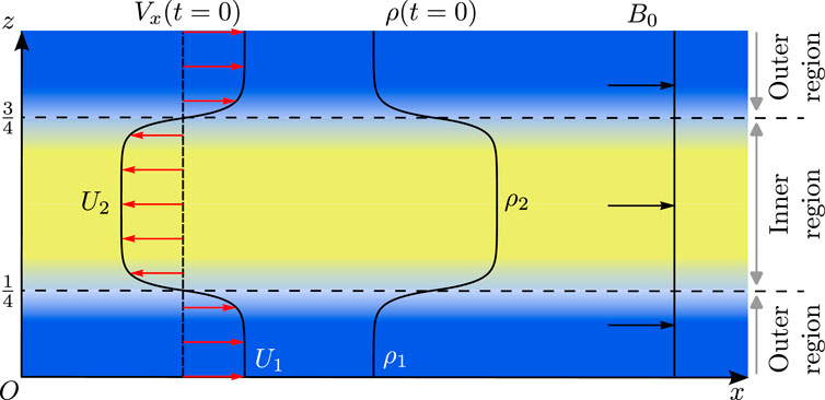
Figure 1. Initial condition for the density field (black) given by (10a), velocity field (red arrows) given by (10b) and uniform horizontal magnetic field (black arrows).

The initial perturbation is inspired from Nykyri et al. [63], with the initial vertical velocity profile being a sum of m_max contributions as follows

where V₀ = 0.01 and each ϕ_m is a random phase that is fixed for all the GAMERA and STRATOSPEC simulations. Two initial conditions are considered in the next sections. The single-mode configuration (SM), with m_min = m_max = 2 (thus only the m = 2 mode is present) and ϕ₂ = 0, so that (11) reduces to the initial condition used in McNally et al. [54]. In the multi-mode configuration (MM), we set m_min = 1 and m_max = 25.

For MHD simulations, an initial uniform magnetic field is imposed parallel to the flow, written as B_x(t = 0) = B₀.

2.4 Objectives and methodology

As mentioned in the introduction, the objective of the present study is to compare GAMERA and STRATOSPEC in the inviscid incompressible limit. This amounts to decrease the Mach number in GAMERA, which solves the compressible Euler equations, and to decrease the diffusion coefficients in STRATOSPEC, which solves the Boussinesq Navier–Stokes equations.

To do so, we first consider the hydrodynamic case in section 3, and both the single-mode and multi-mode initial conditions. We choose to work with small density contrasts between the counter flowing fluids to approach the Boussinesq limit, where the MHD module is available in STRATOSPEC. Hence, starting from the McNally et al. [54] configuration, the Atwood number is decreased from $\mathcal{A}=0.33$ to $\mathcal{A}=0.05$, and this value is kept throughout the study. Still, the large density contrast case for $\mathcal{A}=0.33$ is addressed briefly in the Supplementary Figure S3A to show that the criteria chosen for $\mathcal{A}=0.05$ are still relevant. In addition, even smaller density contrasts are also investigated in the Supplementary Figure S2A, namely, $\mathcal{A}=0.01$, which require more constrained parameters.

In the following analysis, the results of the simulations are compared at three levels: i) qualitatively, ii) 1D profiles in z averaged along the flow direction x, and iii) spectral analysis of the perturbed quantities. Qualitatively, plots of the full density fields are compared at three different dimensionless times, t = 1, 2 and 3 (with t = t^⋆ΔU/L, with t^⋆ the dimensioned time), to assess whether the structures are well reproduced within the two codes GAMERA and STRATOSPEC. Then, averages are performed, at t = 3, along the horizontal, homogeneous, periodic direction x to produce 1D profiles that depend only on the vertical coordinate z. The average of some quantity A along the flow direction is defined as

and the average in the inhomogeneous direction reads

with a′ = A − ⟨A⟩ and ΔL = L_top − L_bottom. For the SM initial condition, due to the top/bottom symmetry of the flow, the average is performed from L_bottom = L/2 to L_top = L, whereas for the MM initial condition, L_bottom = 0. Finally, spectral scale-by-scale comparisons are also provided at t = 3. We write $\widehat{a}$ as the Fourier transform of the fluctuating field a′ and k the modulus of the wavevector k. The various spectra are defined as follows

where a is either v_x, v_z or ρ and S_k is the spherical shell of radius k = |k|. The one-point global variance can then be obtained either from the spherically-averaged spectra or the 1D profiles through

This methodology is used for both the hydrodynamic case in section 3 and the MHD case in section 4.

3 Hydrodynamic regime

We first consider the single-mode case (SM). We investigate the sensitivity of the results in GAMERA to a decreasing Mach number M in order to reach the incompressible limit, along with the effects of decreasing the diffusion coefficients in STRATOSPEC to approach the Euler limit. Afterwards we compare the two codes and extend the comparison to the MM case.

3.1 The inviscid incompressible limit

The density contrast is set to $\mathcal{A}=0.05$, with the averaged density being ρ₀ = (ρ₁ + ρ₂)/2 = 1. To evaluate the effects of compressibility for a given Atwood number, the Mach number M is decreased in GAMERA by gradually increasing the reference pressure from P₀ = 2.5 to P₀ = 80. Results are shown in Figure 2A.

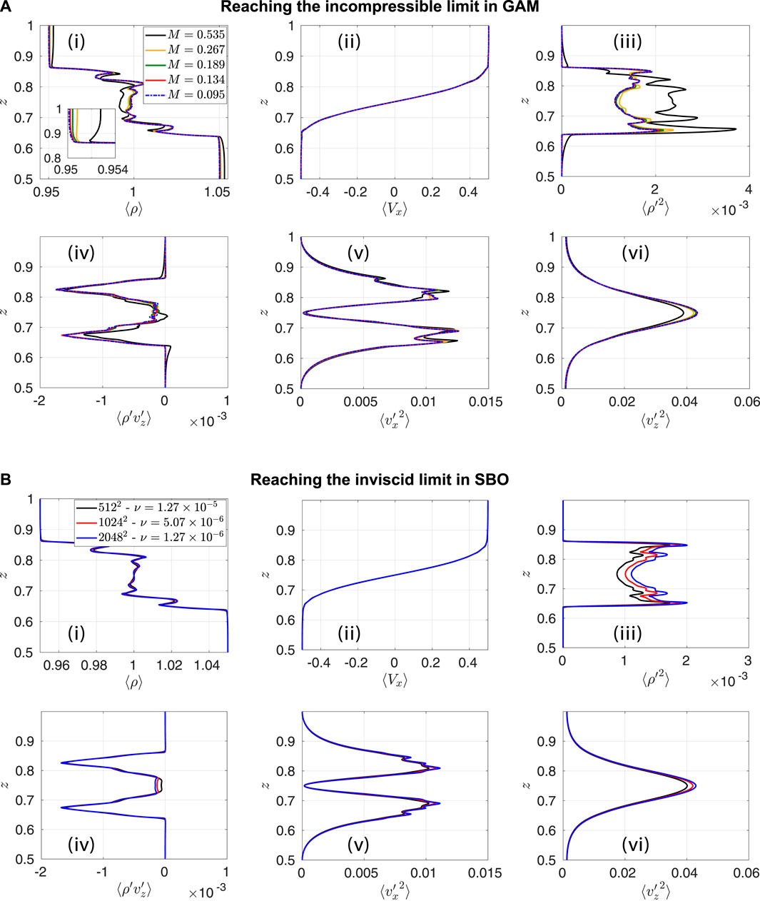
Figure 2. Hydro simulations (1024²) with $\mathcal{A}=0.05$ at t = 3.0: (A) GAM: Decreasing the Mach number M. (B) SBO: Decreasing diffusion coefficients ν = κ (and increasing spatial resolution). (i) Mean density ⟨ρ⟩, (ii) Mean horizontal velocity ⟨V_x⟩, (iii) Density variance ⟨ρ′²⟩, (iv) Vertical mass flux $⟨v_z^{\prime }{\rho }^{\prime }⟩$, (v) Horizontal kinetic energy $⟨{v_x^{\prime }}^2⟩$, (vi) Vertical kinetic energy $⟨{v_z^{\prime }}^2⟩$.

We note that for the largest value of the Mach number, M = 0.535, there are strong discrepancies. The densities of the unmixed fluids depart from their rest values. This can be seen on the mean density ⟨ρ⟩ in Figure 2A, in particular far away from the shear layers, e.g., at z ≃ 0.5 and z ≃ 1.0, and consequently, also on the density variance ⟨ρ′²⟩. Regarding the velocity correlations, the effect of the reference pressure is less pronounced such that the horizontal mean velocity ⟨V_x⟩ is hardly affected. For all quantities, a satisfactory convergence is reached for M ≤ 0.189. Results cannot be distinguished for M = 0.134 and M = 0.095.

A smaller Atwood number is briefly discussed in the Supplementary Figure S2B, and we show that a smaller Mach number must be chosen in GAMERA to ensure a satisfactory comparison with STRATOSPEC. Convergence in terms of spatial resolution for GAMERA is also addressed in the Supplementary Figure S1. We show that resolution with 10,24² and 20,48² points yield almost similar results, so that 20,48² points are chosen for the simulations yielding the main comparisons of this study.

In order to approach the Euler limit (i.e., vanishing bulk viscosity) with the Boussinesq version of STRATOSPEC (SBO), the diffusion coefficients ν = κ are decreased. Conjointly, the number of points is increased to ensure a sufficient spatial resolution. Mean fields in Figure 2B are only slightly affected by a decrease of the diffusion coefficients compared to second-order correlations. The density variance is significantly increased in the turbulent mixing zone when the kinematic viscosity ν is lowered. On the contrary, both horizontal and vertical kinetic energies, along with the vertical mass flux, are less impacted.

In conclusion, for the Atwood number discussed in this study, $\mathcal{A}=0.05$, the inviscid incompressible limit is reached for a resolution of 20,48² points, a Mach number M = 0.134 for GAMERA, and diffusion coefficients of ν = κ = 1.27 × 10⁻⁶ for STRATOSPEC. These parameters are retained throughout the article.

3.2 Single-mode perturbation

The density field for the three codes (GAM, SBO and SVD) is shown for the single-mode perturbation (m = 2) at three different times in Figure 3.

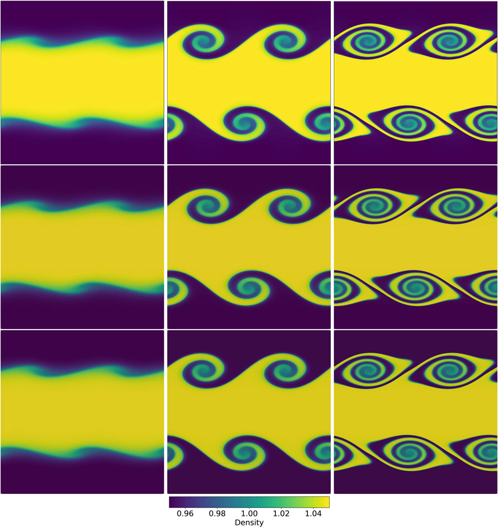
Figure 3. Hydro simulations for GAM (top), SBO (middle) and SVD (bottom) with $\mathcal{A}=0.05$. Density field at t = 1.0, t = 2.0 and t = 3.0.

There is an excellent qualitative agreement, with the presence of rolling structures as the consequence of the mean shear. There are no small-scale shear instabilities: indeed, smaller vortices are observed for large density contrasts due to baroclinic torque [64]. They can be seen in the test case of McNally et al. [54] at $\mathcal{A}=1/3$, and are reproduced with GAMERA for the same Atwood number in Supplementary Figure S3A.

A slight difference can be observed at t = 3 when looking at the bottom vortices, which are slightly shifted towards the left in the GAMERA simulation (top line) compared with the STRATOSPEC-BOUSSINESQ simulation (middle), where the vortices are fixed at the same location. We evaluate a vortex speed along the x-direction of ≃ − 0.012 in GAMERA. The same motion is confirmed with the STRATOSPEC-VARIABLE-DENSITY simulation (bottom line), showing that the advection of the vortices is a non-Boussinesq effect, due to non-zero density contrasts, and not a compressibility effect [65]. Note that if the thickness of the shear layer is neglected, the phase velocity of the KHI can be evaluated as v_ph = (ρ₁U₁ + ρ₂U₂)/(ρ₁ + ρ₂) in the linear regime [1], that would provide a speed of −0.025 in our case. The observed discrepancy can be explained either by finite-thickness effects, or by the fact that the vortices are clearly in the nonlinear phase.

Horizontally averaged profiles are compared in Figure 4A. Looking at GAM (black) and SBO (red) first, slight differences in intensity can be observed for the mean density ⟨ρ⟩ at the center of the shear layer, as well as for the density variance ⟨ρ′²⟩. The horizontal kinetic energy $⟨{v_x^{\prime }}^2⟩$ profiles show some differences around the local maxima, which is the consequence of the Boussinesq simulation SBO yielding perfectly symmetric statistics between the light and heavy fluids. The SVD simulation (blue) in Figure 4A allows one to disentangle the origins of this asymmetry. Indeed, for ⟨ρ⟩, GAM and SVD are superimposed, indicating that the difference with SBO at the center of the mixing region is mainly a non-Boussinesq effect rather than a viscous effect. The same conclusion holds for $⟨{v_x^{\prime }}^2⟩$.

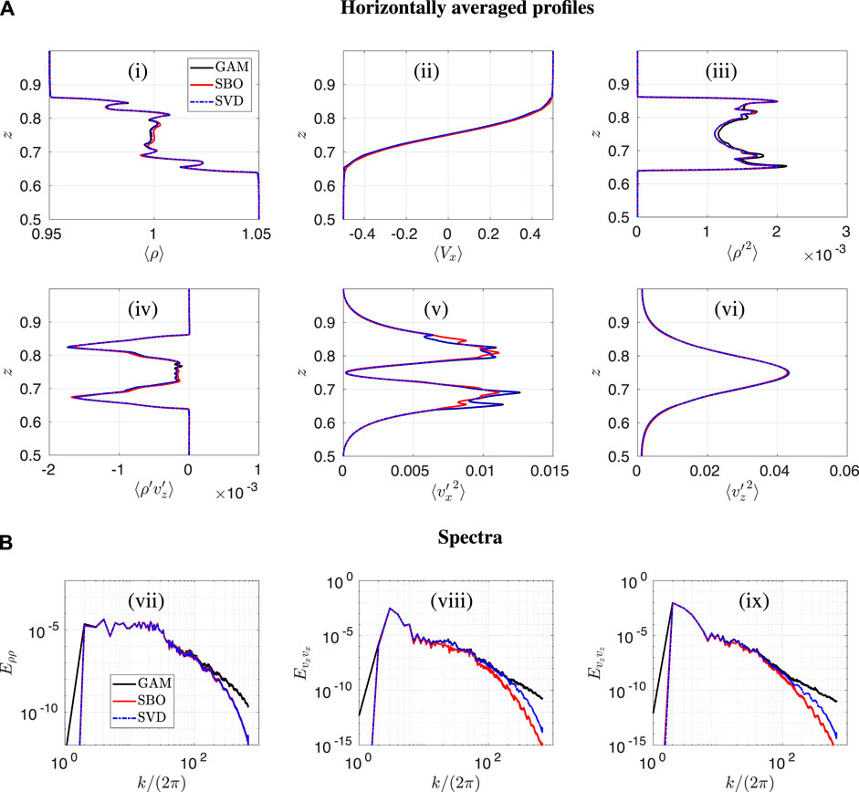
Figure 4. Hydro simulations with $\mathcal{A}=0.05$ at t = 3.0, for GAM, and both SBO and SVD. (A) Horizontally averaged profiles, (B) Spectra. (i) Mean density ⟨ρ⟩, (ii) Mean horizontal velocity ⟨V_x⟩, (iii) Density variance ⟨ρ′²⟩, (iv) Vertical mass flux $⟨v_z^{\prime }{\rho }^{\prime }⟩$, (v) Horizontal kinetic energy $⟨{v_x^{\prime }}^2⟩$, (vi) Vertical kinetic energy $⟨{v_z^{\prime }}^2⟩$, (vii) Spectral density variance E_ρρ, (viii) Spectral horizontal kinetic energy $E_{v_x{v}_x}$, (ix) Spectral vertical kinetic energy $E_{v_z{v}_z}$.

In contrast, SBO and SVD are superimposed for ⟨ρ′²⟩, which shows that this difference with GAM is attributable to non-zero diffusion coefficients in the STRATOSPEC simulations. We investigate further the asymmetry in the GAMERA simulation with a smaller Atwood number in the Supplementary Figure S2B. The asymmetry is less pronounced when lowering the Atwood number, provided the Mach number is jointly decreased, leading to a good agreement between GAM, SBO and SVD. Conversely, at a much larger Atwood number, we show that diffusion smooths the perturbations and regularizes the small-scale shear instabilities in STRATOSPEC (see the Supplementary Figure S3A).

We conclude from the mean fields ⟨ρ⟩ and ⟨V_x⟩ that the large-scale flows are well reproduced by the three codes. The second-order correlations ⟨ρ′²⟩, $⟨{v_x^{\prime }}^2⟩$, $⟨{v_z^{\prime }}^2⟩$ and $⟨v_z^{\prime }{\rho }^{\prime }⟩$ illustrate that some differences persist at the smallest scales, which are mainly due to viscosity and diffusion in STRATOSPEC.

Spectra of the second-order moments, which include both the information at large and small scales, are shown in Figure 4B and support this point. Excellent agreement is found between the codes for the large scales (small k) while there are more discrepancies at small scales (large k). Most of the small-scale differences can be explained by a stronger dissipation in STRATOSPEC due to non-zero diffusion coefficients. The comparison with the Variable-Density formulation of STRATOSPEC also shows that differences at intermediate scales are only due to non-Boussinesq effects, as already pointed out in Figure 4A.

3.3 Multi-mode perturbation

We continue the analysis of the hydrodynamic KHI by considering the multi-mode case (MM) given in Eq. 11 with m_min = 1 and m_max = 25 modes. The density fields of the GAMERA and STRATOSPEC simulations are first presented in Figure 5. The agreement is excellent, showing that nonlinearities are well captured by both codes. Contrary to the SM case, MM perturbations create a top/bottom asymmetry, already visible at t = 2. Indeed, the merging process, where small vortices are absorbed by bigger ones, results in larger vortices of various shapes and does not proceed at the same rate at the two shear layers.

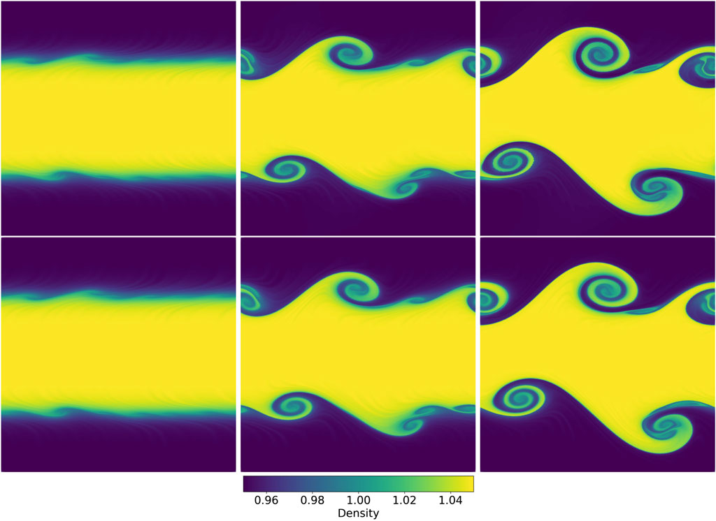
Figure 5. Multi-mode hydro simulations (2048²) for GAM (top) and SBO (bottom) with $\mathcal{A}=0.05$. Density field at t = 1.0, t = 2.0 and t = 2.5.

The asymmetry of the flow requires computation of the 1D horizontally-averaged profiles over the whole domain z ∈ [0, 1] as done in Figure 6A. The overall agreement is again satisfactory. The strong asymmetry between the top and bottom parts in the horizontal kinetic energy $⟨{v_x^{\prime }}^2⟩$ is well captured and is attributed to the two bottom vortices which have different heights.

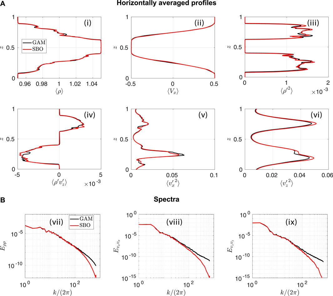
Figure 6. Multi-mode hydro simulations with $\mathcal{A}=0.05$ at t = 2.5, for GAM and SBO. (A) Horizontally averaged profiles, (B) Spectra. (i) Mean density ⟨ρ⟩, (ii) Mean horizontal velocity ⟨V_x⟩, (iii) Density variance ⟨ρ′²⟩, (iv) Vertical mass flux $⟨v_z^{\prime }{\rho }^{\prime }⟩$, (v) Horizontal kinetic energy $⟨{v_x^{\prime }}^2⟩$, (vi) Vertical kinetic energy $⟨{v_z^{\prime }}^2⟩$, (vii) Spectral density variance E_ρρ, (viii) Spectral horizontal kinetic energy $E_{v_x{v}_x}$, (ix) Spectral vertical kinetic energy $E_{v_z{v}_z}$.

Finally, the density and velocity spectra for the MM case are presented in Figure 6B. Similar to the SM perturbation, large scales are superimposed while more discrepancies persist at small scales. Nevertheless, the overall agreement is better as the flow becomes less sensitive to diffusion at smaller scales due to the interaction of several modes.

4 MHD regime

We now extend the analysis to MHD, considering an initial uniform mean magnetic field B_x(t = 0) = B₀ = 0.2 parallel to the flow. Considering ΔU/B₀ as the ratio of shear velocity upon Alfvén velocity, we expect a flow still dominated by sheared vortices, although a mean magnetic field parallel to the flow may stabilize the KH instability [1]. Discussions regarding the linear stability of the magnetic KH and the effects of compressibility are postponed in section 5.

For this part, we keep the settings used in the previous section (resolution, Mach number and diffusion coefficients) and employ a similar analysis: after qualitatively describing the effects of a tangential mean magnetic field upon the developing KHI, the GAMERA and STRATOSPEC codes are compared for the SM and MM initial conditions. The case of a lower mean magnetic field (B₀ = 0.1) is discussed in the Supplementary Figure S4.

4.1 Single-mode perturbation

The effects of gradually increasing the mean magnetic field magnitude from B₀ = 0 to B₀ = 0.2 is shown in Figure 7A. Compared with the hydrodynamic case (B₀ = 0), the vortices are progressively stretched and flatten when B₀ increases, with the same orientation compared to the interface. Till B₀ = 0.1 (corresponding to $M_a^{\Vert }=10$), vortices fold the original interface. For the largest intensity, B₀ = 0.2, exactly at the threshold $M_a^{\Vert }=5$ for having folded structures [35], the vortices have almost vanished and only thin filaments of density close to ρ₀ remain. This case will be analyzed further below.

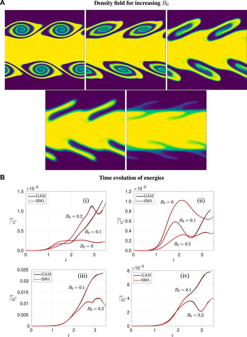
Figure 7. MHD simulations (2048²) for GAM and SBO with $\mathcal{A}=0.05$. (A) Increasing mean magnetic field B₀ ∈ [0; 0.05; 0.10; 0.15; 0.20] at t = 3.0 for GAM. (B) Time evolution of (i) horizontal kinetic energy $\overline{{v_x^{\prime }}^2}$, (ii) vertical kinetic energy $\overline{{v_z^{\prime }}^2}$, (iii) horizontal magnetic energy $\overline{{b_x^{\prime }}^2}$, (iv) vertical magnetic energy $\overline{{b_z^{\prime }}^2}$.

Conversion, through the mean shear and magnetic field, of vertical kinetic energy $\overline{{v_z^{\prime }}^2}$ into horizontal kinetic energy $\overline{{v_x^{\prime }}^2}$, both computed according to (13), can be analyzed by considering their time evolution shown in Figure 7B. Beyond the good agreement between GAM and SBO simulations, we observe an increasing horizontal kinetic energy at the expense of the vertical kinetic energy as the magnitude of B₀ increases. This corresponds to the damping of the vortices and their stretching in the flow direction. The induced magnetic energies in Figure 7B decrease with increasing B₀ because structures are more aligned with the flow and less distorted. Note that the magnetic energy in the flow direction $\overline{{b_x^{\prime }}^2}$ is always stronger than in the transverse direction.

We pursue the investigation of the single-mode magnetized KHI for the case B₀ = 0.2. The density fields are shown at three different times in Figure 8, with a nice agreement between the STRATOSPEC and GAMERA simulations. Differences with the hydrodynamic case are significant. The magnetic field acts as a tension that tends to stabilize the interface and prevent the rolling of the structures. At t = 2, unlike the hydrodynamic case (Figure 3), there is almost no rolling. At t = 3, only thin filaments survive. Indeed, being exactly at the threshold for rolling, the magnetic tension seems to be sufficiently strong for hindering the folding at t = 2, and even for causing its regression at t = 3. This is particularly visible in the bottom row of Figure 8, where magnetic field lines have been drawn in white for the GAMERA simulation. The line corresponding to the bluish plasma, clearly separating the yellow and dark-blue regions, is almost folded at t = 2 but goes back to a nearly straight line at t = 3. We also note that there is a very good correspondence between the field lines and the density structures that, in the incompressible limit, are generated by the sole advection. This means that the ideal MHD frozen-in law is well respected during the simulation duration. In fact, there is no sign of magnetic island along the magnetic inversion layers that have been created in correspondence with the thin filaments. Numerical diffusivity is thus sufficiently low for preventing the development of Type II VIR [36].

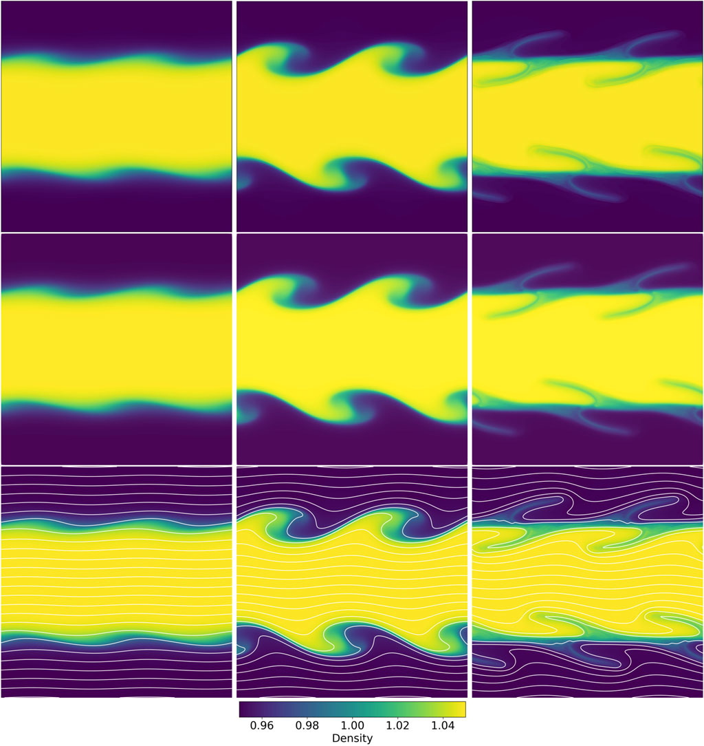
Figure 8. MHD simulations (2048²) for GAM (top) and SBO (bottom) with $\mathcal{A}=0.05$ and B₀ = 0.2. Density field at t = 1.0, t = 2.0 and t = 3.0. The last row highlights the magnetic field lines in the GAM simulation.

Regarding the horizontally-averaged profiles, there is an excellent agreement between GAM and SBO for the mean fields in Figure 9. For ⟨ρ⟩, there is almost no mixing, with a flat profile between ρ₁ and ρ₂, whereas a wider mixing region with a mean density ρ₀ exists in the hydrodynamic case (see Figure 4A). This is consistent with the magnetic field preventing mixing through the development of small scales. The mean horizontal velocity ⟨V_x⟩ is distorted due to the thin elongated filaments detaching from the interface. The induced mean magnetic field ⟨B_x⟩ has significantly evolved compared with its initial constant state. It is vanishing in the inner regions where the thin filaments form, at z ≃ 0.68 and z ≃ 0.82, and much stronger inside the thin mixing layer. Regarding second-order correlations, we now also include the horizontal and vertical magnetic energies, $⟨{b_x^{\prime }}^2⟩$ and $⟨{b_z^{\prime }}^2⟩$, in Figure 9. There is an overall good agreement for all statistics between the GAM and SBO simulations, with sharp variations being well captured. We also confirm this good agreement for a mean magnetic field twice as small (B₀ = 0.1) for which vortices are much more distorted (see 1D profiles in Supplementary Figure S4.

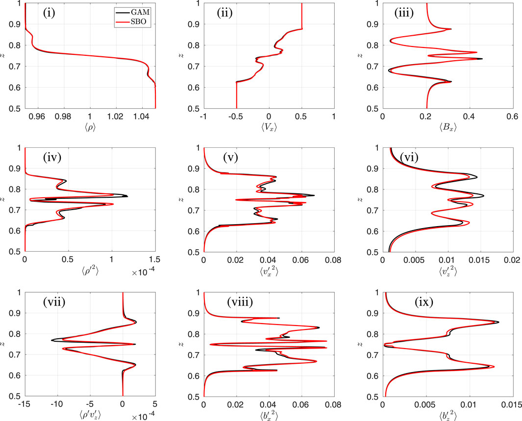
Figure 9. MHD simulations (2048²) with $\mathcal{A}=0.05$ and B₀ = 0.2 at t =3.0, for GAM and SBO. Horizontally averaged profiles of (i) Mean density ⟨ρ⟩, (ii) Mean horizontal velocity ⟨V_x⟩, (iii) Mean horizontal magnetic field ⟨B_x⟩ (iv) Density variance ⟨ρ′²⟩, (v) Horizontal kinetic energy $⟨{v_x^{\prime }}^2⟩$, (vi) Vertical kinetic energy $⟨{v_z^{\prime }}^2⟩$, (vii) Vertical mass flux $⟨v_z^{\prime }{\rho }^{\prime }⟩$, (viii) Horizontal magnetic energy $⟨{b_x^{\prime }}^2⟩$, (ix) Vertical magnetic energy $⟨{b_z^{\prime }}^2⟩$.

Spectra of the various correlations are presented in Figure 10. Similar to the purely hydrodynamic case, we find excellent agreement at large scales. However, smaller scales (k/(2π) > 30) are found to be quite different for E_ρρ. This is attributed to more mixing in STRATOSPEC due to non-zero diffusion coefficients, which significantly reduces the variance. Since the MHD case is less distorted (the mean magnetic field smooths the small scales), the velocity and magnetic spectra remain very close, with an agreement at both large and small scales. The spectral index in the inertial range is roughly between −2 and −2.5.

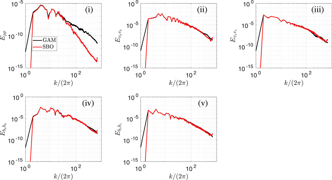
Figure 10. MHD simulations (2048²) with $\mathcal{A}=0.05$ and B₀ = 0.2 at t = 3.0, for GAM and SBO. Spectra of (i) density variance E_ρρ, (ii) horizontal kinetic energy $E_{v_x{v}_x}$, (iii) vertical kinetic energy $E_{v_z{v}_z}$, (iv) horizontal magnetic energy $E_{b_x{b}_x}$, (v) vertical magnetic energy $E_{b_z{b}_z}$.

4.2 Multi-mode perturbation with B₀ = 0.2

We address the MM perturbation in the MHD case with B₀ = 0.2 in Figure 11. Even though small scales are suppressed quite early by the mean magnetic field, some large vortices survive. The top/bottom asymmetry in the shear layers is quite visible.

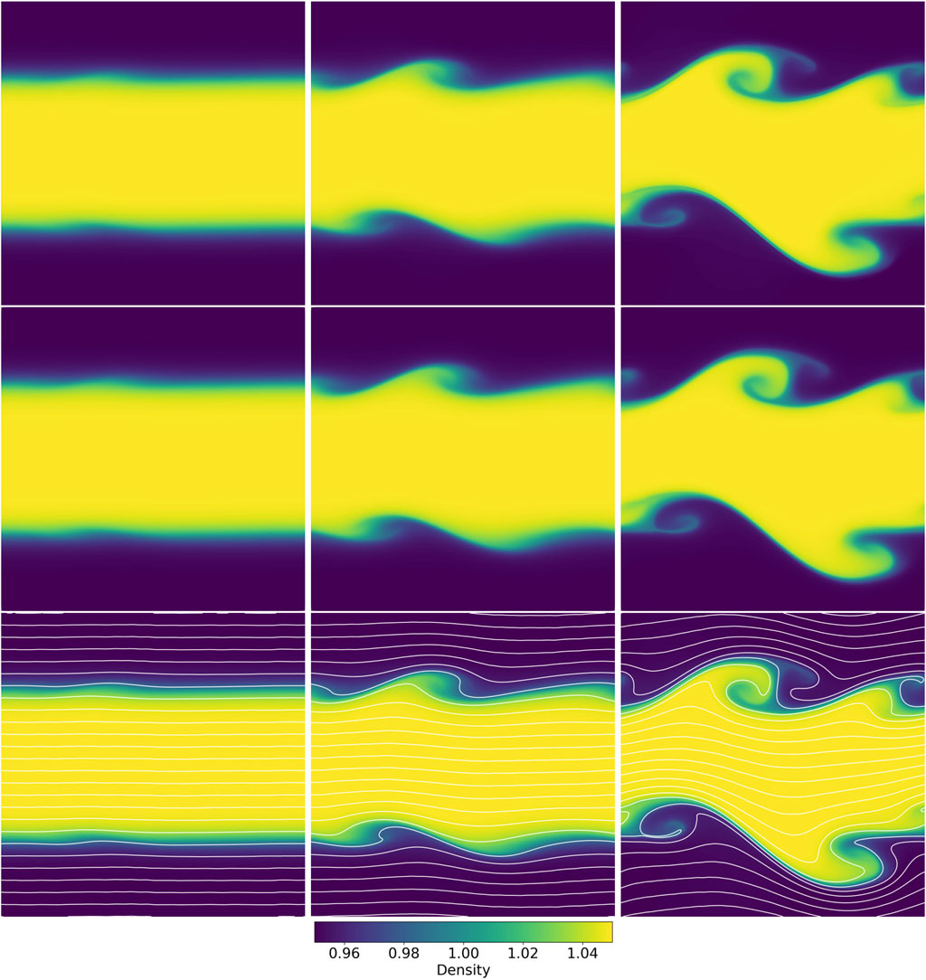
Figure 11. Multi-mode MHD simulations (2048²) for GAM (top) and SBO (bottom) with $\mathcal{A}=0.05$ and B₀ = 0.2. Density field at t = 1.0, t = 2.0 and t = 3.0. The last row highlights the magnetic field lines in the GAM simulation.

The rolling is less pronounced than in the purely hydrodynamic case (see Figure 5) but it is more active than in the SM counterpart (Figure 8) with rolls being able to develop. It is worth noticing that the non-linear evolution of the KHI can be strongly influenced by the number of modes that have been perturbed at t = 0, even if some of them are growing slowy, or not growing at all, during the linear phase. This point has been raised in Matsumoto and Seki [66], where the vortex merging at large scales strongly depensd on the perturbation of stable small-scale modes. Similarly, SM or MM initial conditions lead to a completely different non-linear evolution in Nakamura and Fujimoto [67] and in Faganello et al. [68].

Like in SM case, we note a very good agreement between field lines and density structures (Figure 11, bottom row). Moreover, no sign of Type II VIR is present, even if very thin magnetic inversion layers have been generated by the vortex motion, like the one at x ∼ 0.15, x ∼ 0.3, at t = 3.

The agreement between GAM and SBO for the horizontally-averaged profiles of density, velocity and magnetic fields is quite remarkable, as shown in Figure 12. Small differences in amplitude for the various variances are observed and are attributed to non-zero viscosity in STRATOSPEC simulations. The top/bottom asymmetry is well recovered for all quantities including the variances. Modulations of the induced horizontal mean magnetic field ⟨B_x⟩ are less intense than in the SM case.

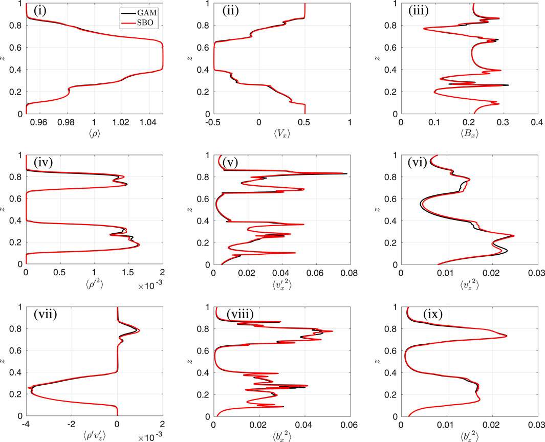
Figure 12. Multi-mode MHD simulations (2048²) with $\mathcal{A}=0.05$ and B₀ = 0.2 at t = 3.0, for GAM and SBO. Horizontally averaged profiles of (i) Mean density ⟨ρ⟩, (ii) Mean horizontal velocity ⟨V_x⟩, (iii) Mean horizontal magnetic field ⟨B_x⟩ (iv) Density variance ⟨ρ′²⟩, (v) Horizontal kinetic energy $⟨{v_x^{\prime }}^2⟩$, (vi) Vertical kinetic energy $⟨{v_z^{\prime }}^2⟩$, (vii) Vertical mass flux $⟨v_z^{\prime }{\rho }^{\prime }⟩$, (viii) Horizontal magnetic energy $⟨{b_x^{\prime }}^2⟩$, (ix) Vertical magnetic energy $⟨{b_z^{\prime }}^2⟩$.

Finally, spectra of the various second-order correlations are shown in Figure 13. Compared with the MM purely hydrodynamic case (Figure 6B), the magnetic field effect and smoother profiles lead to an agreement up to larger k, namely, k/(2π) > 200. Similar to the SM perturbation, all spectra of GAM and SBO are in excellent agreement (up to k/(2π) > 200), except for the density variance departing at k/(2π) ≃ 30. The agreement at large and intermediate scales is quite convincing. The spectral index in the inertial range is once again between −2 and −2.5: we make no further comment on this since 2D turbulence induced by single-mode or multi-mode perturbations is quite singular.

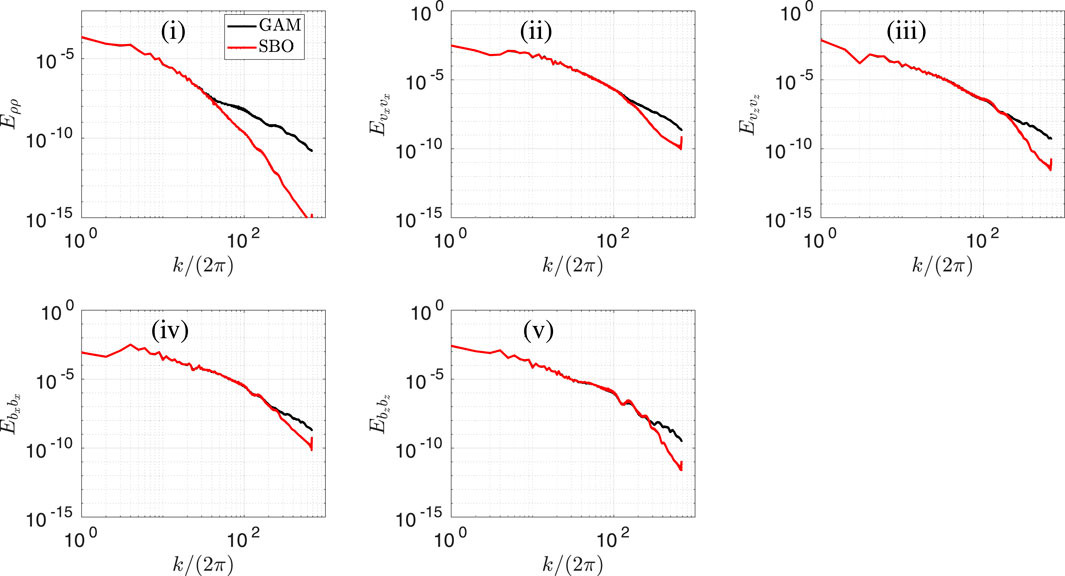
Figure 13. Multi-mode MHD simulations (2048²) with $\mathcal{A}=0.05$ and B₀ = 0.2 at t = 3.0, for GAM and SBO. Spectra of (i) density variance E_ρρ, (ii) horizontal kinetic energy $E_{v_x{v}_x}$, (iii) vertical kinetic energy $E_{v_z{v}_z}$, (iv) horizontal magnetic energy $E_{b_x{b}_x}$, (v) vertical magnetic energy $E_{b_z{b}_z}$.

5 Growth rate analysis in the linear regime

The magnetized KHI is studied in the seminal article by Miura and Pritchett [57] for a compressible plasma in super-Alfvénic conditions. These authors show that for a magnetic field parallel to the flow, with a fixed Mach number M, the growth rate of the perturbation reduces with decreasing Alfvénic Mach number M_a = ΔU/B₀ (see their Figure 4 with line plots reproduced below). With the present notations, since B₀ is parallel to the flow, $M_a=M_a^{\Vert }$.

Here in GAMERA, we define an initial small perturbation in order to remain in the linear stability regime. Following Miura and Pritchett [57], we consider a single-mode velocity perturbation V_z of small amplitude V₀ = 1 × 10⁻⁶, such that V₀/λ ≪ΔU/L, with λ = 2π/k_x the wavelength of the perturbation, and a uniform background density, leading to $\mathcal{A}=0$. The velocity profile in the x direction is set to be a hyperbolic tangent of steepness a = 0.025. A series of simulations was done for M = 1.0 and k_x = 2mπ (m = 1–5). Note that depending upon the profile chosen for the background shear flow, the stability curves can be quite different [69].

Growth rates are computed from simulations ran with GAMERA. The numerical extraction of the growth rates is shown in Figure 14A, in which the energy of the dominant Fourier mode E_z,k, normalized by its initial value, is plotted with respect to time. For each simulation, we perform a least square fit leading to the exponential growth rate, shown for k_x = 6π in Figure 14A. We start with the compressible case at M = 1, for which normalized growth rates (dots) are shown in Figure 14B and compared with the profiles of Miura and Pritchett (solid lines). Error bars are computed from the standard deviation of the least square fits, and are displayed on both sides of the growth rate value, forming a star shape as the standard deviation is always very small. The standard deviation increases when the wavenumber comes closer to the stability criterion. Differences are small enough to consider this method as fully valid and applicable. The agreement between GAMERA and Miura and Pritchett is very satisfactory. A 5%–20% error remains for k_x = 2π regardless of the Alfvénic Mach number M_a.

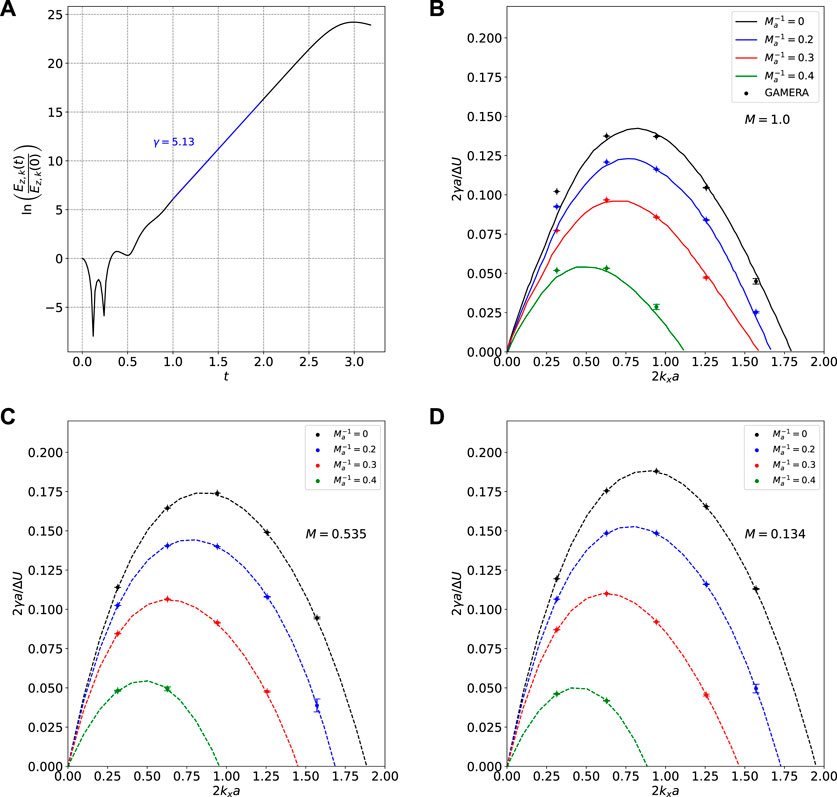
Figure 14. (A) Time evolution of the Fourier component associated to the vertical kinetic energy (black) for a single-mode perturbation (k_x = 6π) with B₀ = 0. The least square fit is plotted in blue with the associated growth rate. (B) Normalized growth rates as function of the normalized wavenumber for $\mathcal{A}=0$ and M = 1.0. Comparison with Miura and Pritchett (solid lines) for different Alfvénic Mach numbers M_a. (C) and (D) Normalized growth rates for $\mathcal{A}=0.05$ with M = 0.535 and M = 0.134, respectively. A polynomial interpolation function is added to better represent the bell shaped structure (dashed lines). The coefficient are tabulated in the Supplementary Material.

The effect of compressibility in the magnetized KHI is now highlighted by using the same methodology and reducing gradually the Mach number to M = 0.535 and then to M = 0.134. The latter value has been shown to reach the incompressible limit in the previous sections. Simulations are performed at $\mathcal{A}=0.05$. We checked that changing the Atwood number from $\mathcal{A}=0$ to $\mathcal{A}=0.05$, at fixed Mach numbers, does not significantly modify the growth rates. Hence, the results in Figures 14C,D can be compared with those at M = 1 in Figure 14B.

Growth rates are also presented in Figure 15 for various k_x modes and plotted with respect to the Alfvénic Mach number in order to better show the effects of compressibility. Quadratic interpolation curves are added when possible (see Supplementary Table S1 for details), starting at M_a = 2 in order to respect the instability criterion M ≤ 2 < M_a [57]. Otherwise, growth rates are linearly interpolated, for instance for k_x = 8π.

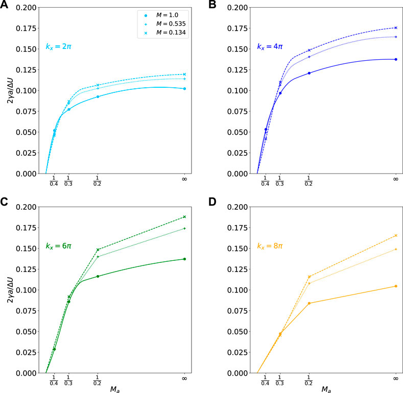
Figure 15. Normalized growth rate as function of the Alfvénic Mach numbers M_a and Mach numbers M (different symbols), for various horizontal wavenumber: (A) k_x = 2π, (B) k_x = 4π, (C) k_x = 6π, and (D) k_x = 8π.

The growth rate increases significantly when the Mach number is decreased from M = 1 to M = 0.535, showing the damping by compressibility of the KHI. Growth rates increase to a lesser extent when further decreasing the Mach number from M = 0.535 to M = 0.134, showing that compressibility effects become negligible and justifying a posteriori the choice of this value for the previous comparisons with STRATOSPEC. Growth rates show more differences at larger k_x mode.

Irrespective of the Mach number, the growth rates decrease when the mean magnetic field intensity B₀ is increased, or similarly when the inverse Alfvénic Mach number increases. This explains why, in Figure 7A, structures are more damped when B₀ increases. This is shown as well in Figure 15, where growth rates become closer to each other as the Alfvénic Mach number decreases, and differences vanish for M_a < 3. Hence, from the point of view of the linear stability, the incompressible limit is more easily satisfied in the presence of intense magnetic fields.

6 Conclusion

We address the effects of compressibility, diffusion, and magnetohydrodynamics upon the development of 2D Kelvin–Helmholtz instabilities for conditions prevailing in space and fusion applications. To this purpose, a numerical study is performed with two state of the art codes, GAMERA and STRATOSPEC. GAMERA solves the compressible MHD Euler equations with high-order reconstruction in arbitrary nonorthogonal curvilinear coordinates. STRATOSPEC solves the MHD Navier–Stokes equations in the Boussinesq limit (SBO) with a pseudo-spectral method of infinite order. Our 2D Kelvin–Helmholtz test case is greatly inspired by McNally et al. [54], in which two counter flows of different densities interact with each other and mix. The initial interfaces have smooth steepness, which prevents spurious numerical issues when dealing with sharp gradients. The original density contrast is lowered to $\mathcal{A}=0.05$ to approach the Boussinesq limit.

The common limit between the two codes is the inviscid incompressible one. We reach it by decreasing the Mach number in GAMERA, and decreasing the diffusion coefficients in STRATOSPEC. With these parameters appropriately chosen, along with the spatial resolution, single-mode and multi-mode perturbations are investigated, with and without a mean magnetic field parallel to the flow.

The analysis is then performed with three diagnostics. First, the overall topology of the developing vorticies is qualitatively assessed with the instantaneous 2D density fields. Second, 1D profiles of horizontally averaged quantities reveal differences of two different origins: i) small scales are smoothed out by diffusion in STRATOSPEC, causing for example, the density variance to be less intense than in GAMERA. ii) the asymmetry between the vortex development at the two different shear layers persists, even at small density contrasts such as $\mathcal{A}=0.05$. The correct displacement of the vortices is well reproduced with the Variable-Density version of STRATOSPEC, as well as with GAMERA. Finally, spectra of the fluctuating fields encompass information at all scales, with an almost perfect agreement at the largest ones, and some discrepancies between the two codes at the smallest scales, especially for the density variance. Differences are amplified in the MHD cases, possibly because structures are flatter, so that diffusion effects become more important in STRATOSPEC compared to vortex stretching.

We also note a good agreement between the density and magnetic structures in the MHD case. This is expected since, in the incompressible limit, the initial inhomogeneous density is just advected by the fluid velocity, as it is the case for magnetic field lines in the ideal MHD regime.

To summarize, this study shows that the inviscid incompressible limit can be approached by the two codes. Increasing the amplitude of the mean magnetic field damps the vortices, which eventually become long and thin filaments advected by the mean flow. Viscosity and diffusion could be further decreased in STRATOSPEC, but at the expense of increasing spatial resolution. Non-Boussinesq effects could also be reduced in GAMERA by further decreasing the Atwood number (down to $\mathcal{A}=0.01$, see Supplementary Material), which in turn requires to decrease the Mach number in GAMERA, and hence the CFL condition down to a prohibitive cost. Conversely, we show that the Mach number chosen for the study remains relevant to maintain the incompressible regime in the hydrodynamic case even for large density contrasts ($\mathcal{A}=1/3$, see the Supplementary Material). In that case, the molecular diffusion becomes critical regarding the development of small-scale secondary vortices, which are damped in STRATOSPEC.

Finally, in the framework of the linear stability analysis, and in a manner reminiscent to Miura and Pritchett [57], we demonstrated that the exponential growth rates of initial small perturbations in the magnetic KHI are damped both by compressibility and increasing mean magnetic field intensity. The growth rates diagrams are essential for comparing and understanding KHI features encountered in highly complex environments such as laser experiments or the Earth’s magnetosphere, for which they are hard to be measured or numerically computed.

Studies of KHI can benefit from considering also the development of resonant flow instability (RFI). RFI can occur for velocity shears significantly below the Kelvin–Helmholtz instability threshold for pressureless plasma [70], such as coronal plumes, as well as in the incompressible limit [71]. RFI becomes important when the length scale of the Alfvén speed variation is larger than the length scale of the flow speed variation [72]. In the present study, the length scales of the flow and Alfvén velocity gradients are equal, which limits the development of RFI. For further discussions on RFI, the reader is referred to the recent article by Kim et al. [73] and references therein.

This work paves the way to promising studies at larger density contrasts and Mach numbers. The proposed approach helps to disentangle which mechanisms are truly a consequence of compressibility, or were already present in the incompressible limit. The method can be extended to other canonical flows, such as buoyancy-driven ones like the Rayleigh–Taylor instability, also relevant for laser and astrophysical considerations.

Data availability statement

The original contributions presented in the study are included in the article/Supplementary Material, further inquiries can be directed to the corresponding authors.

Author contributions

AB: Conceptualization, Data curation, Formal Analysis, Investigation, Methodology, Project administration, Resources, Software, Validation, Visualization, Writing–original draft, Writing–review and editing. J-FR: Conceptualization, Data curation, Formal Analysis, Funding acquisition, Investigation, Methodology, Project administration, Resources, Software, Supervision, Validation, Visualization, Writing–original draft, Writing–review and editing. AM: Investigation, Methodology, Software, Supervision, Validation, Writing–review and editing. B-JG: Conceptualization, Investigation, Methodology, Software, Supervision, Validation, Writing–review and editing. GP: Data curation, Methodology, Software, Validation, Writing–review and editing. MC: Software, Writing–review and editing. HE-R: Conceptualization, Formal Analysis, Methodology, Supervision, Validation, Writing–review and editing. MF: Formal Analysis, Investigation, Methodology, Validation, Visualization, Writing–review and editing. VM: Formal Analysis, Methodology, Software, Validation, Writing–review and editing. KS: Methodology, Software, Writing–review and editing. AU: Funding acquisition, Methodology, Software, Writing–review and editing. JL: Methodology, Writing–review and editing. AR: Methodology, Writing–review and editing. Victorien Bouffetier: Writing–review and editing. LC: Writing–review and editing. HS: Writing–review and editing. OH: Writing–review and editing. VS: Funding acquisition, Writing–review and editing. AC: Funding acquisition, Writing–review and editing.

Funding

The author(s) declare financial support was received for the research, authorship, and/or publication of this article. NIF Discovery Science (DS) project P-000794—Calming Kelvin-Helmholtz Instability with pre-imposed B field: bringing Solar Wind and Magnetosphere Physics into the laboratory. AM, KS, VM, AK, and JL were supported by the NASA DRIVE Science Center for Geospace Storms (CGS) under award 80NSSC22M0163.

Acknowledgments

All authors thank the NIF Discovery Science Program. We thank the NASA DRIVE Science Center for Geospace Storms (CGS). J-FR, AU, AM and MC thank the International Space Science Institute (ISSI) in Bern, through ISSI International Team project #477 (Radiation Belt Physics From Top To Bottom).

Conflict of interest

The authors declare that the research was conducted in the absence of any commercial or financial relationships that could be construed as a potential conflict of interest.

The author(s) declared that they were an editorial board member of Frontiers, at the time of submission. This had no impact on the peer review process and the final decision

Publisher’s note

All claims expressed in this article are solely those of the authors and do not necessarily represent those of their affiliated organizations, or those of the publisher, the editors and the reviewers. Any product that may be evaluated in this article, or claim that may be made by its manufacturer, is not guaranteed or endorsed by the publisher.

Supplementary material

The Supplementary Material for this article can be found online at: https://www.frontiersin.org/articles/10.3389/fphy.2024.1383514/full#supplementary-material

References

1. Chandrasekhar S. Hydrodynamic and hydromagnetic stability. United Kingdom: Oxford University Press (1961).
2. Lobanov A, Zensus J. A cosmic double helix in the archetypical quasar 3c273. Science (2001) 294:128–31. doi:10.1126/science.1063239
3. Li X, Zhang J, Yang S, Hou Y, Erdélyi R. Observing kelvin–helmholtz instability in solar blowout jet. Scientific Rep (2018) 8:8136. doi:10.1038/s41598-018-26581-4
4. Ershkovich AI. Kelvin-helmholtz instability in type-1 comet tails and associated phenomena. Space Sci Rev (1980) 25:3–34. doi:10.1007/bf00200796
5. Johnson JR, Wing S, Delamere PA. Kelvin helmholtz instability in planetary magnetospheres. Space Sci Rev (2014) 184:1–31. doi:10.1007/s11214-014-0085-z
6. Foullon C, Verwichte E, Nakariakov VM, Nykyri K, Farrugia CJ. Magnetic kelvin–helmholtz instability at the sun. Astrophysical J Lett (2011) 729:L8. doi:10.1088/2041-8205/729/1/l8
7. Hasegawa H, Fujimoto M, Phan T-D, Reme H, Balogh A, Dunlop M, et al. Transport of solar wind into earth’s magnetosphere through rolled-up kelvin–helmholtz vortices. Nature (2004) 430:755–8. doi:10.1038/nature02799
8. Haaland S, Runov A, Artemyev A, Angelopoulos V. Characteristics of the flank magnetopause: themis observations. J Geophys Res Space Phys (2019) 124:3421–35. doi:10.1029/2019ja026459
9. Walsh B, Thomas E, Hwang K-J, Baker J, Ruohoniemi J, Bonnell a. W. Dense plasma and kelvin-helmholtz waves at earth’s dayside magnetopause. J Geophys Res Space Phys (2015) 120:5560–73. doi:10.1002/2015ja021014
10. Merkin V, Lyon J, Claudepierre S. Kelvin-helmholtz instability of the magnetospheric boundary in a three-dimensional global mhd simulation during northward imf conditions. J Geophys Res Space Phys (2013) 118:5478–96. doi:10.1002/jgra.50520
11. Sorathia K, Merkin V, Panov E, Zhang B, Lyon J, Garretson J, et al. Ballooning-interchange instability in the near-earth plasma sheet and auroral beads: global magnetospheric modeling at the limit of the mhd approximation. Geophys Res Lett (2020) 47:e2020GL088227. doi:10.1029/2020gl088227
12. Michael A, Sorathia K, Merkin V, Nykyri K, Burkholder B, Ma X, et al. Modeling kelvin-helmholtz instability at the high-latitude boundary layer in a global magnetosphere simulation. Geophys Res Lett (2021) 48:e2021GL094002. doi:10.1029/2021gl094002
13. Mostafavi P, Merkin VG, Provornikova E, Sorathia K, Arge C, Garretson J. High-resolution simulations of the inner heliosphere in search of the kelvin–helmholtz waves. Astrophysical J (2022) 925:181. doi:10.3847/1538-4357/ac3fb4
14. Hwang K-J, Wang C-P, Nykyri K, Hasegawa H, Tapley MB, Burch JL, et al. Kelvin-helmholtz instability-driven magnetopause dynamics as turbulent pathway for the solar wind-magnetosphere coupling and the flank-central plasma sheet communication. Front Astron Space Sci (2023) 10:1151869. doi:10.3389/fspas.2023.1151869
15. Faganello M, Califano F, Pegoraro F, Retinò A. Kelvin-helmholtz vortices and double mid-latitude reconnection at the earth’s magnetopause: comparison between observations and simulations. Europhysics Lett (2014) 107:19001. doi:10.1209/0295-5075/107/19001
16. Eriksson S, Lavraud B, Wilder F, Stawarz J, Giles B, Burch J, et al. Magnetospheric multiscale observations of magnetic reconnection associated with kelvin-helmholtz waves. Geophys Res Lett (2016) 43:5606–15. doi:10.1002/2016gl068783
17. Nakamura T, Hasegawa H, Daughton W, Eriksson S, Li WY, Nakamura R. Turbulent mass transfer caused by vortex induced reconnection in collisionless magnetospheric plasmas. Nat Commun (2017) 8:1582. doi:10.1038/s41467-017-01579-0
18. Rossi C, Califano F, Retinò A, Sorriso-Valvo L, Henri P, Servidio S, et al. Two-fluid numerical simulations of turbulence inside kelvin-helmholtz vortices: intermittency and reconnecting current sheets. Phys Plasmas (2015) 22:122303. doi:10.1063/1.4936795
19. Stawarz J, Eriksson S, Wilder F, Ergun R, Schwartz S, Pouquet A, et al. Observations of turbulence in a kelvin-helmholtz event on 8 september 2015 by the magnetospheric multiscale mission. J Geophys Res Space Phys (2016) 121:11–021. doi:10.1002/2016ja023458
20. Di Mare F, Sorriso-Valvo L, Retinò A, Malara F, Hasegawa H. Evolution of turbulence in the kelvin–helmholtz instability in the terrestrial magnetopause. Atmosphere (2019) 10:561. doi:10.3390/atmos10090561
21. Faganello M, Califano F. Magnetized Kelvin–Helmholtz instability: theory and simulations in the earth’s magnetosphere context. J Plasma Phys (2017) 83:535830601. doi:10.1017/s0022377817000770
22. Garbet X, Fenzi C, Capes H, Devynck P, Antar G. Kelvin–Helmholtz instabilities in tokamak edge plasmas. Phys Plasmas (1999) 6:3955–65. doi:10.1063/1.873659
23. Chapman I, Brown S, Kemp R, Walkden N. Toroidal velocity shear kelvin–helmholtz instabilities in strongly rotating tokamak plasmas. Nucl Fusion (2012) 52:042005. doi:10.1088/0029-5515/52/4/042005
24. Myra JR, D’Ippolito DA, Russell DA, Umansky MV, Baver DA. Analytical and numerical study of the transverse kelvin–helmholtz instability in tokamak edge plasmas. J Plasma Phys (2016) 82:905820210. doi:10.1017/S0022377816000301
25. Vandenboomgaerde M, Bonnefille M, Gauthier P. The kelvin-helmholtz instability in national ignition facility hohlraums as a source of gold-gas mixing. Phys Plasmas (2016) 23:052704. doi:10.1063/1.4948468
26. Hurricane O, Hansen J, Robey H, Remington B, Bono M, Harding E, et al. A high energy density shock driven kelvin–helmholtz shear layer experiment. Phys Plasmas (2009) 16:056305. doi:10.1063/1.3096790
27. Harding E, Hansen J, Hurricane O, Drake R, Robey H, Kuranz C, et al. Observation of a kelvin-helmholtz instability in a high-energy-density plasma on the omega laser. Phys Rev Lett (2009) 103:045005. doi:10.1103/physrevlett.103.045005
28. Smalyuk V, Hansen J, Hurricane O, Langstaff G, Martinez D, Park H-S, et al. Experimental observations of turbulent mixing due to kelvin–helmholtz instability on the omega laser facility. Phys Plasmas (2012) 19:092702. doi:10.1063/1.4752015
29. Walsh C, Crilly A, Chittenden J. Magnetized directly-driven icf capsules: increased instability growth from non-uniform laser drive. Nucl Fusion (2020) 60:106006. doi:10.1088/1741-4326/abab52
30. Malamud G, Shimony A, Wan WC, Di Stefano CA, Elbaz Y, Kuranz CC, et al. A design of a two-dimensional, supersonic KH experiment on OMEGA-EP. High Energ Density Phys (2013) 9:672–86. doi:10.1016/j.hedp.2013.06.002
31. Malamud G, Elgin L, Handy T, Huntington C, Drake RP, Shvarts D, et al. Design of a single-mode Rayleigh–taylor instability experiment in the highly nonlinear regime. High Energ Density Phys (2019) 32:18–30. doi:10.1016/j.hedp.2019.04.004
32. Barbeau Z, Raman K, Manuel M, Nagel S, Shivamoggi B. Design of a high energy density experiment to measure the suppression of hydrodynamic instability in an applied magnetic field. Phys Plasmas (2022) 29:012306. doi:10.1063/5.0067124
33. Di Stefano CA, Malamud G, Henry De Frahan MT, Kuranz CC, Shimony A, Klein SR, et al. Observation and modeling of mixing-layer development in high-energy-density, blast-wave-driven shear flow. Phys Plasmas (2014) 21. doi:10.1063/1.4872223
34. Kent A. Stability of laminar magnetofluid flow along a parallel magnetic field. J Plasma Phys (1968) 2:543–56. doi:10.1017/S0022377800004025
35. Jones TW, Gaalaas JB, Ryu D, Frank A. The mhd kelvin-helmholtz instability. ii. the roles of weak and oblique fields in planar flows. Astrophysical J (1997) 482:230–44. doi:10.1086/304145
36. Otto A, Fairfield DH. Kelvin-helmholtz instability at the magnetotail boundary: mhd simulation and comparison with geotail observations. J Geophys Res Space Phys (2000) 105:21175–90. doi:10.1029/1999JA000312
37. Faganello M, Califano F, Pegoraro F. Being on time in magnetic reconnection. New J Phys (2009) 11:063008. doi:10.1088/1367-2630/11/6/063008
38. Blumen W. Shear layer instability of an inviscid compressible fluid. J Fluid Mech (1970) 40:769–81. doi:10.1017/S0022112070000435
39. Blumen W, Drazin PG, Billings DF. Shear layer instability of an inviscid compressible fluid. part 2. J Fluid Mech (1975) 71:305–16. doi:10.1017/S0022112075002595
40. Miura A. Kelvin-helmholtz instability for supersonic shear flow at the magnetospheric boundary. Geophys Res Lett (1990) 17:749–52. doi:10.1029/GL017i006p00749
41. Kobayashi Y, Kato M, Nakamura K, Nakamura T, Fujimoto M. The structure of kelvin–helmholtz vortices with super-sonic flow. Adv Space Res (2008) 41:1325–30. doi:10.1016/j.asr.2007.04.016
42. Palermo F, Faganello M, Califano F, Pegoraro F, Le Contel O. Compressible kelvin-helmholtz instability in supermagnetosonic regimes. J Geophys Res Space Phys (2011) 116. doi:10.1029/2010JA016400
43. Soler R, Ballester J. Theory of fluid instabilities in partially ionized plasmas: an overview. Front Astron Space Sci (2022) 9:789083. doi:10.3389/fspas.2022.789083
44. Galtier S. Wave turbulence in incompressible hall magnetohydrodynamics. J Plasma Phys (2006) 72:721–69. doi:10.1017/s0022377806004521
45. Sahraoui F, Galtier S, Belmont G. On waves in incompressible hall magnetohydrodynamics. J plasma Phys (2007) 73:723–30. doi:10.1017/s0022377806006180
46. Manzini D, Sahraoui F, Califano F, Ferrand R. Local energy transfer and dissipation in incompressible hall magnetohydrodynamic turbulence: the coarse-graining approach. Phys Rev E (2022) 106:035202. doi:10.1103/physreve.106.035202
47. Martínez-Gómez D, Soler R, Terradas J. Onset of the kelvin-helmholtz instability in partially ionized magnetic flux tubes. Astron Astrophysics (2015) 578:A104. doi:10.1051/0004-6361/201525785
48. Lyon J, Fedder J, Mobarry C. The lyon–fedder–mobarry (lfm) global mhd magnetospheric simulation code. J Atmos Solar-Terrestrial Phys (2004) 66:1333–50. doi:10.1016/j.jastp.2004.03.020
49. Merkin VG, Panov EV, Sorathia K, Ukhorskiy AY. Contribution of bursty bulk flows to the global dipolarization of the magnetotail during an isolated substorm. J Geophys Res Space Phys (2019) 124:8647–68. doi:10.1029/2019ja026872
50. Zhang B, Sorathia K, Lyon J, Merkin V, Garretson J, Wiltberger M. GAMERA: a three-dimensional finite-volume MHD solver for non-orthogonal curvilinear geometries. Astrophysical J Suppl Ser (2019) 244:20. doi:10.3847/1538-4365/ab3a4c
51. Briard A, Gostiaux L, Gréa B-J. The turbulent Faraday instability in miscible fluids. J Fluid Mech (2020) 883:A57. doi:10.1017/jfm.2019.920
52. Briard A, Gréa B-J, Nguyen F. Growth rate of the turbulent magnetic Rayleigh-Taylor instability. Phys Rev E (2022) 106:065201. doi:10.1103/physreve.106.065201
53. Briard A, Gréa B-J, Nguyen F. Turbulent mixing in the vertical magnetic Rayleigh–Taylor instability. J Fluid Mech (2024) 979:A8. doi:10.1017/jfm.2023.1053
54. McNally C, Lyra W, Passy J-C. A well-posed Kelvin–Helmholtz instability test and comparison. Astrophysical J Suppl Ser (2012) 201:18. doi:10.1088/0067-0049/201/2/18
55. Lecoanet D, McCourt M, Quataert E, Burns KJ, Vasil GM, Oishi JS, et al. A validated non-linear kelvin–helmholtz benchmark for numerical hydrodynamics. Monthly Notices R Astronomical Soc (2016) 455:4274–88. doi:10.1093/mnras/stv2564
56. Soler R, Diaz A, Ballester J, Goossens M. Kelvin–Helmholtz instability in partialliy ionized compressible plasmas. Astrophysical J (2012) 749:163. doi:10.1088/0004-637x/749/2/163
57. Miura A, Pritchett P. Nonlocal stability analysis of the mhd kelvin-helmholtz instability in a compressible plasma. J Geophys Res Space Phys (1982) 87:7431–44. doi:10.1029/ja087ia09p07431
58. Ong RSB, Roderick N. On the kelvin-helmholtz instability of the earth’s magnetopause. Planet Space Sci (1972) 20:1–10. doi:10.1016/0032-0633(72)90135-3
59. Viciconte G, Gréa B-J, Godeferd F, Arnault P, Cléroin J. Sudden diffusion of turbulent mixing layers in weakly coupled plasmas under compression. Phys Rev E (2019) 100:063205. doi:10.1103/physreve.100.063205
60. Pekurovsky D. P3DFFT: a framework for parallel computations of Fourier transforms in three dimensions. J Scientific Comput (2012) 34:C192–C209. doi:10.1137/11082748x
61. Viciconte G. Turbulent mixing driven by variable density and transport coefficients effects. Phd thesis. Lyon: Université de Lyon (2019).
62. Evans CR, Hawley JF. Simulation of magnetohydrodynamic flows-a constrained transport method. Astrophysical J (1988) 332:659–77. doi:10.1086/166684
63. Nykyri K, Ma X, Dimmock A, Otto A, Osmane A. Influence of velocity fluctuations on the kelvin-helmholtz instability and its associated mass transport. J Geophys Res Space Phys (2017) 122:9489–512. doi:10.1002/2017ja024374
64. Reinaud J, Joly L, Chassaing P. The baroclinic secondary instability of the two-dimensional shear layer. Phys Fluids (2000) 12:2489–505. doi:10.1063/1.1289503
65. Dimotakis PE. Two-dimensional shear-layer entrainment. AIAA J (1986) 24:1791–6. doi:10.2514/3.9525
66. Matsumoto Y, Seki K. Formation of a broad plasma turbulent layer by forward and inverse energy cascades of the kelvin–helmholtz instability. J Geophys Res Space Phys (2010) 115. doi:10.1029/2009JA014637
67. Nakamura TKM, Fujimoto M. Magnetic effects on the coalescence of kelvin-helmholtz vortices. Phys Rev Lett (2008) 101:165002. doi:10.1103/PhysRevLett.101.165002
68. Faganello M, Califano F, Pegoraro F. Time window for magnetic reconnection in plasma configurations with velocity shear. Phys Rev Lett (2008) 101:175003. doi:10.1103/PhysRevLett.101.175003
69. Berlok T, Pfrommer C. On the kelvin–helmholtz instability with smooth initial conditions–linear theory and simulations. Monthly Notices R Astronomical Soc (2019) 485:908–23. doi:10.1093/mnras/stz379
70. Andries J, Tirry W, Goossens M. Modified kelvin-helmholtz instabilities and resonant flow instabilities in a one-dimensional coronal plume model: results for plasma β= 0. Astrophysical J (2000) 531:561–70. doi:10.1086/308430
71. Hollweg JV, Yang G, Cadez V, Gakovic B. Surface waves in an incompressible fluid-resonant instability due to velocity shear. Astrophysical J (1990) 349:335–44. doi:10.1086/168317
72. Taroyan Y, Erdélyi R. Resonant surface waves and instabilities in finite β plasmas. Phys Plasmas (2003) 10:266–76. doi:10.1063/1.1532741
Keywords: Kelvin–Helmholtz instability, MHD, numerical simulations, scale-by-scale comparisons, growth rates
Citation: Briard A, Ripoll J-F, Michael A, Gréa B-J, Peyrichon G, Cosmides M, El-Rabii H, Faganello M, Merkin VG, Sorathia KA, Ukhorskiy AY, Lyon JG, Retino A, Bouffetier V, Ceurvorst L, Sio H, Hurricane OA, Smalyuk VA and Casner A (2024) The inviscid incompressible limit of Kelvin–Helmholtz instability for plasmas. Front. Phys. 12:1383514. doi: 10.3389/fphy.2024.1383514
Received: 07 February 2024; Accepted: 22 March 2024;
Published: 19 April 2024.
Edited by:
Rui A. P. Perdigão, Meteoceanics Institute for Complex System Science, United StatesReviewed by:
Ram Prasad Prajapati, Jawaharlal Nehru University, IndiaRobertus Erdelyi, The University of Sheffield, United Kingdom
Copyright © 2024 Briard, Ripoll, Michael, Gréa, Peyrichon, Cosmides, El-Rabii, Faganello, Merkin, Sorathia, Ukhorskiy, Lyon, Retino, Bouffetier, Ceurvorst, Sio, Hurricane, Smalyuk and Casner. This is an open-access article distributed under the terms of the Creative Commons Attribution License (CC BY). The use, distribution or reproduction in other forums is permitted, provided the original author(s) and the copyright owner(s) are credited and that the original publication in this journal is cited, in accordance with accepted academic practice. No use, distribution or reproduction is permitted which does not comply with these terms.
*Correspondence: A. Briard, antoine.briard@cea.fr; J.-F. Ripoll, jean-francois.ripoll@cea.fr