A Coupled, Global/Local Finite Element Methodology to Evaluate the Fatigue Life of Flexible Risers Attached to Floating Platforms for Deepwater Offshore Oil Production

Abstract

This study introduces a Finite Element (FE) hybrid methodology for analyzing deepwater offshore oil and gas floating production systems. In these systems, flexible risers convey the production and are connected to a balcony on one side of the platform. The proposed methodology couples, in a cost-effective manner, the hydrodynamic model of the platform with the FE model that represents the risers and the mooring lines, considering all nonlinear dynamic interactions. The results obtained and the associated computational performance are then compared with those from traditional uncoupled analyses, which may present inaccurate results for deepwater scenarios, and from fully coupled analyses that may demand high computational costs. Moreover, particular attention is dedicated to integrating global and local stress analyses to calculate the fatigue resistance of the flexible riser. The results demonstrate that the coupled global analyses adequately capture the asymmetric behavior due to all risers being connected to one of the sides of the platform, thus resulting in a more accurate distribution of fatigue damage when compared to the uncoupled methodology. Also, fatigue life is significantly affected by adequately considering the coupling effects.

1. Introduction

Deepwater offshore oil production activities have been performed mainly by floating production systems (FPS) such as ship-shaped Floating Production, Storage, and Offloading (FPSOs) vessels. They offer a relatively cost-effective and fast solution with high storage capacity so that they can operate in remote fields. For instance, in Brazilian offshore pre-salt areas, this type of vessel has been installed at an average depth of 2000 m and 300 km from the coast [1].

In FPSs, slender structures such as risers, umbilicals, and mooring lines connect the bottom of the sea to the platform, configuring the typical deepwater offshore scenario for oil and gas exploitation. These structures are designed considering 10-year and 100-year extreme environmental conditions of wave, wind, and current and their directional distributions. Besides extreme conditions, typical operational scenarios must also be addressed due to structural fatigue concerns.

The first decision in FPSO deployment usually is to choose between a “spread mooring” system, where an array of mooring lines distributed along the vessel hull restrains its rotation (nowadays, generally associated with a riser balcony), and a “turret mooring” system that allows the vessel to weathervane according to prevailing waves, winds, and currents, effectively reducing overall mooring forces. The spread mooring configuration costs are usually lower than those related to turret moorings; also, spread moorings are typically best suited to locations in West Africa and Brazil [2] due to the predominance of a current direction during the year.

Regarding the risers that convey the oil and gas production to an FPSO, selecting the best configuration for deepwater is also heavily influenced by the geographical location and the prevailing weather conditions, considering the environmental challenges that each region presents. Still, the main objective is ensuring optimal system performance and reliability. Usually, the free-hanging flexible riser shown in Figure 1 has been the preferred choice in moderate offshore environments typical of Brazilian scenarios.

Despite their relatively higher cost, flexible risers are considered a suitable solution in those scenarios compared to steel (rigid) risers because they are somewhat simpler to transport and install. In addition, their complex, multilayered structure ensures low bending stiffness, high compliance, and high resistance to torsion, tension, and internal and external pressures. The mechanical characteristics of a flexible pipe are guaranteed by a set of metallic and polymeric layers, as shown in Figure 2: an inner carcass to prevent internal collapse, a pressure armor, and two or four layers of helical wires, named tensile armors, that are counter-wound. The polymeric layers, in turn, minimize friction between the metallic layers, prevent seawater ingress and internal fluid leakage, and insulate the pipe [3].

Generally, riser analysis comprises two analysis types. The first is the global analysis, which involves modeling the entire length of the pipe (as shown in Figure 1), typically with three-dimensional beam finite elements, to obtain the loads acting in its cross-sections. The second is the local analysis, which evaluates the stresses induced in each layer considering the loads calculated in the global analyses.

In deepwater scenarios, the top section of the riser is subjected to high tensile loads, which combine with significant bending moments. Moreover, the contact region with the seabed touchdown zone (TDZ) experiences high hydrostatic pressures associated with bending moments. Altogether, this scenario is highly favorable to fatigue failure that may be aggravated by stress corrosion cracking (SCC) [6]. Indeed, the performance of flexible risers in the offshore fatigue context is not a recent concern [7,8,9]; codes, standards, and a set of theoretical studies have been developed to establish the best practices for flexible risers analysis [3,10,11]. The main difficulties consist of knowing their design limits and, more importantly, determining the loads to which they would be subjected in service.

In this context, the numerical simulation of such systems employing FE-based methods is an essential tool for their design. Particular attention should be dedicated to the nonlinear dynamic interactions between the vessel and the lines connected to it. Traditionally, on shallower waters, global analyses using uncoupled models, where the vessel and the lines are analyzed separately, provided good approximations for efforts and displacements. However, in deepwater scenarios, the effects of the elastic, damping, and inertial forces of the risers and mooring lines begin to interfere with the vessel response, indicating that coupled analysis would be required [12]. Moreover, variations in damping ratio and mass coefficients concerning vessel motion were reported across distinct coupling levels. The concern with such nonlinear dynamic interactions began when [13] observed that for TLPs (tension leg platforms), the higher the water depth, the greater the influence of the nonlinear behavior of the tendons on the vessel. This study already noted that the motions of each system element (platform, mooring tendons, and production lines) could not be considered independently. Further on [12], the behavior of a platform with turret-type mooring for different water depths was studied, including a deepwater scenario (2000 m). The uncoupled analysis of these vessels proved inaccurate when calculating the vessel offsets for low-frequency wave motions and tension on lines.

Innovative approaches to riser and mooring analysis methodologies, encompassing different levels of design integration, have been investigated in [14] where an accurate semi-coupled approach was presented that offered good results when considering a full nonlinear static coupled analysis to find the mean equilibrium position of the FPS, which was then used to calculate the new degrees of freedom of the vessel. After that, dynamic analyses were performed.

The present work proposes to take the next step towards a coupled dynamic analysis methodology, initiated by [15,16], but this time focusing on the fatigue context. Special attention is dedicated to applications on deepwater and ultra-deepwater scenarios involving FPSOs with numerous mooring lines and risers featuring a riser balcony on one side. For such applications, ref. [15] highlighted the substantial influence of nonlinear stiffness, inertia, and particularly damping effects from the lines on the hull dynamic behavior. Those studies have shown that the motions of the top connections of the risers are influenced by the coupling of the lines to the hull, resulting in asymmetric responses of vertical displacement in these top connections and an asymmetric response of the roll motion. These responses are due to the high number of lines in the riser balcony and the ultra-deepwater context, which increases the structures’ self-weight and damping. Moreover, this coupling effect gains prominence since coupled roll motion RAOs (Response Amplitude Operators) generated through time-domain coupled analyses using FE software exhibit notably lower energy content and asymmetry, which cannot be observed in traditional uncoupled analysis. Thus, as the roll motion is critical for the fatigue effects in the lines, together with the heave motions and tension, this work investigates the influence of the coupling of the roll and heave motions on the fatigue life of flexible risers in such deepwater scenarios.

Another aspect addressed in this work is that, in general, coupled analysis studies have been conducted with a global approach, observing the hull behavior, global dynamic tensions, and moments on the lines. Now, having noted the asymmetric behavior of the FPSO with a riser balcony reported in the previous studies and considering the coupling of the hull with the mooring lines and risers, the objective here is to investigate the fatigue damage with local models that consider the different layers of the risers’ cross-section via coupled and uncoupled analyses. The goal is to demonstrate that the asymmetric behavior captured by the coupled analyses results in a different distribution of fatigue damage compared to the uncoupled methodology.

The remainder of this article is organized as follows. Initially, Section 2 describes the classical uncoupled methodology for the global analysis of FPSs and then outlines the primary concepts of coupled methodologies. Section 3 addresses the local analysis of flexible risers by revisiting a previously proposed approach to calculate fatigue damage in the tensile armors of these structures. Section 4 states the methodology proposed in this study, and Section 5 delineates the case study that illustrates the application of the coupled methodology for fatigue life calculation, taking an actual spread moored FPSO operating in a deepwater scenario. Finally, Section 6 discusses the results obtained, and Section 7 states the main conclusions of this study.

2. Review of Methodologies for the Global Analysis of FPSs

2.1. Classical Procedure for Riser Analysis: Uncoupled Methodology

Uncoupled methodologies use numerical tools based on formulations that do not consider the nonlinear interaction between the hull and the lines. The first step involves analyses to obtain the vessel’s motions in its six degrees of freedom, i.e., the three translations (Surge, Sway, and Heave) and the three rotations (Roll, Pitch, and Yaw). In these analyses, the mooring lines and risers are represented by simplified models (e.g., as scalar coefficients), obtaining vessel motions in terms of static offsets, low frequency (LF), and wave frequency (WF) components. The latter is expressed as transfer functions or Response Amplitude Operators (RAOs) [17,18,19], a set of coefficients that linearly correlates the first-order vessel motions with the wave amplitudes, assuming a linear relationship between the wave amplitude and the resulting wave forces or motions for each given wave period. The vessel RAOs are usually calculated in the frequency domain, employing programs based on radiation/diffraction models. The vessel is modeled as a three-dimensional rigid body assuming small unsteady motions relative to the body’s wavelength and relevant length scales. The panel method models the body surface and calculates the body’s hydrodynamic pressure, loads, and motions, as well as the pressure and velocity in the fluid domain [20].

To calculate the RAO of forces and moments $S_{RAO}\left({\omega }_f\right)$ resulting from first-order effects, wave spectra $S_{\zeta }\left({\omega }_f\right)$ combined with the transfer function $RAO\left({\omega }_f\right)$ are used as in Equation (1).

$$S_{RAO}\left({\omega }_f\right)=S_{\zeta }\left({\omega }_f\right)RAO{\left({\omega }_f\right)}^2$$

(1)

The wave energy spectrum is the distribution that represents each frequency’s contribution to an irregular sea’s energy. Figure 3 gives a graphical interpretation of the meaning of a wave spectrum and how it relates to the waves. The irregular wave history in the time domain, $\zeta \left(t\right)$, function of the time t, can be expressed via Fourier series analysis as the sum of many regular wave components, each with its frequency, amplitude, and random phase in the frequency domain. The value ½$\zeta {\left({\omega }_f\right)}^2/\Delta {\omega }_f$, associated with each wave component is plotted vertically, representing the wave energy spectrum $S_{\zeta }\left({\omega }_f\right)$.

The second step of the uncoupled methodology consists of performing nonlinear global dynamic FE analyses to obtain tensions, bending moments, and curvatures of the mooring lines and risers modeled. In these analyses, the lines are represented by three-dimensional truss and/or beam finite elements, and the vessel motions obtained in the first stage are introduced as boundary conditions at the connection points of the lines, calculated from the obtained RAOs. Moreover, such analyses are usually performed in the time domain to correctly represent all nonlinear effects, including the drag forces. The dynamic analyses may be simplified by considering deterministic regular waves or irregular sea-states defined by spectral models such as the JONSWAP spectrum discretized in the time domain by an ensemble of regular wave components.

This uncoupled approach has been widely used in extreme, fatigue, and interference analyses due to its easy implementation and low computational cost. It may give acceptable results for shallow water scenarios, where nonlinear restoring forces, damping, and inertia effects from mooring lines and risers have a minor influence on the vessel motions. However, it involves several simplifications, mainly disregarding the nonlinear interaction between vessels and lines. Refs. [18,19] have pointed out that the advance of offshore oil production towards ultra-deepwater scenarios would require more accurate design methodologies in which each component of a floating system (vessel, mooring lines, and risers) no longer can be considered separately but rather as a coupled system, confirming pioneering studies, such as those presented by [12,22]. That is, increasing water depth leads to increased contribution of the mass and damping of mooring lines and risers [17]. Hence, the system’s overall behavior is dictated not only by the hydrodynamic behavior of the hull but also by its interaction with the hydrodynamic–structural behavior of the lines.

2.2. Coupled Methodology

The lines and hull are no longer considered separate domains in fully coupled analysis methodologies. Coupled analyses can simultaneously generate the vessel motions and the structural response of mooring lines and risers; they are based on a full-time-domain method and a rigorous representation of the lines by FE models to consider all nonlinearities involved in the system’s dynamic response. Moreover, coupled models implicitly evaluate these components under the same environmental loading matrix.

Jacob et al. [16] studied alternative coupling formulations named “weak coupling” WkC and “strong coupling” StC. The WkC formulation focuses on the equations of motion of the vessel: the coupling between the hydrodynamic model of the vessel and the hydrodynamic/structural model of the lines is performed by forces acting on the right-hand side of the vessel equations. At each time step of the time integration of the hull equation, the body motions are prescribed at the connection nodes of the FE models for each line. The resulting forces at the top of the lines are then applied to the platform.

On the other hand, in the StC formulation, the FE matrices of mass, damping, and stiffness from all mooring lines and risers are assembled, forming a single set of equations and a single global matrix, where the hull is considered as a “node” of the model. The whole system (hull and lines) is treated as a single domain, and the system of equations is solved using a single numerical integration algorithm.

However, since it groups all the finite element meshes of the lines, the StC formulation requires a significant amount of computational memory, having a high computational cost. Thus, this work considers the WkC formulation since previous studies [16] have demonstrated that it presents accurate results for typical applications of FPSs.

2.3. Hybrid Methodologies

Strictly speaking, the so-called “fully coupled” methodology involves using highly refined FE meshes to provide detailed structural responses, demanding high computational effort. Hence, the goal of obtaining a balance between accuracy and computational efficiency may be reached by “hybrid” methodologies.

Different procedures may comprise these methodologies, such as using an equivalent vertical cylinder to represent the drag forces from risers and mooring lines [23]. Another hybrid approach employs static analysis on a three-dimensional FE model to derive a restoring force vs. displacement curve for calibrating traditional springs, simulating riser elastic stiffness. Further options involve incorporating coefficients calibrated through decay tests to emulate line damping and the introduction of scalar mass coefficients to approximate the system mass. A “coupled motion analysis” has been proposed in [22]. The risers are modeled with coarse FE meshes that are not refined enough to provide a detailed structural response but are sufficient to obtain more accurate vessel motions considering the nonlinear dynamic interaction between the vessel and lines. Subsequently, uncoupled analyses of each riser are performed, applying these vessel motions and using refined FE meshes to obtain their structural response. Additionally, ref. [14] presents a semi-coupled three-step procedure to reduce computational costs in coupled methodologies.

2.4. Formulation of the Equations of Motion

In this work, the coupled analyses have been performed using the in-house, non-commercial SITUA-Prosim nonlinear dynamic analysis program [16]. This section summarizes the formulation of the equations of motion that describe the vessel (represented as a rigid body defined by its global geometric, hydrodynamic, and mass properties) and its mooring lines and risers (represented by FE meshes of three-dimensional truss and beam finite elements), and the solution methods employed to solve the equations.

The exact large amplitude equations of motion of the vessel [24] comprise the following set of twelve first-order differential equations, with the unknown variables being $\mathit{v}$, $\mathit{x}$, $\mathit{\omega }$ and $\mathit{\theta }$, which are three-dimensional vectors with, respectively, the translational and angular components of velocities and the position of the body as functions of time:

$$\frac{d\mathit{v}}{dt}={\mathbf{M}}_h^{-1}\mathit{f}, \frac{d\mathit{\omega }}{dt}={\mathbf{I}}_h^{-1}\left[\mathit{m}-\mathit{\omega }\times \left({\mathbf{I}}_{\mathit{h}}\mathit{\omega }\right)\right]$$

(2)

$$\frac{d\mathit{x}}{dt}=\mathit{v}, \frac{d\mathit{\theta }}{dt}={\mathbf{B}}^{-1}\mathit{\omega }$$

(3)

In these equations, the 3 × 3 matrices ${\mathbf{M}}_h$, ${\mathbf{I}}_h$ and $\mathbf{B}$ are, in this order, the diagonal matrix with the dry mass of the hull, the moments and products of inertia, and a rotation matrix with sines and cosines of the Euler angles. Vectors $\mathit{f}$ and $\mathit{m}$ are the external forces and moments due to the environmental loadings of wind, wave, and current. The hydrodynamic wave forces are evaluated by taking the first-order exciting force RAOs and the second-order drift force coefficients, both available from previous analyses employing the WAMIT [20] hydrodynamic radiation/diffraction analysis program. As demonstrated in [16], Equations (2) and (3) can be rewritten in the following matrix form:

$$\left[\begin{array}{cc}{\mathbf{M}}_{\mathrm{h}}+{\mathbf{A}}_{\mathrm{h}}& {\mathbf{B}}_{\mathrm{h}}\\ {\mathbf{C}}_{\mathrm{h}}& {\mathbf{I}}_{\mathrm{h}}+{\mathbf{D}}_{\mathrm{h}}\end{array}\right]\left\{\begin{array}{c}\frac{d\mathit{v}}{dt}\\ \frac{d\mathit{\omega }}{dt}\end{array}\right\}=\left\{\begin{array}{c}{\mathit{f}}_1\\ {\mathit{m}}_1-\mathit{\omega }\times \left({\mathbf{I}}_{\mathrm{h}}\mathit{\omega }\right)\end{array}\right\}$$

(4)

where ${\mathit{f}}_1$ and ${\mathit{m}}_1$ are force and moment terms that depend on the position, velocity, and time but do not depend on the acceleration. The matrix in brackets on the left is the augmented 6 × 6 global mass matrix. Besides submatrices ${\mathit{M}}_h$ and ${\mathit{I}}_h$, it also includes the added mass matrices ${\mathit{A}}_h$ and ${\mathit{D}}_h$ updated at every time step, and the coupling added mass terms ${\mathit{B}}_h$ and ${\mathit{C}}_h$. Equation (4) may be solved using different dynamic solution algorithms, including the fourth-order Runge–Kutta time integration method.

The nonlinear structural dynamic behavior of the mooring lines and risers is described by equations of motion that arise from the Finite Element (FE) spatial discretization. These can be written as follows, the unknowns being acceleration, velocity, and displacement vectors $\ddot{\mathit{u}}\left(t\right)$, $\dot{\mathit{u}}\left(t\right)$ and $\mathit{u}\left(t\right)$ (each component corresponding to a degree of freedom of the FE mesh):

$$\mathbf{M}\ddot{\mathit{u}}\left(t\right)+\mathbf{C}\dot{\mathit{u}}\left(t\right)+\mathbf{R}\left[\mathit{u}\left(t\right)\right]=\mathit{F}\left(\mathit{u},t\right)$$

(5)

where $\mathit{C}$ is the Rayleigh proportional damping matrix $\mathit{C}={\propto }_m\mathit{M}+{\alpha }_k\mathit{K}$, [25] a linear combination of the global mass and stiffness matrices $\mathit{M}$ and $\mathit{K}$ assembled from the contributions of the corresponding matrices from each finite element; $\mathit{R}\left(u\right)$ is a vector of internal elastic forces (nonlinear function of the unknown displacements $\mathit{u}$); and $\mathit{F}$ is the vector of external loads (also a nonlinear function of $\mathit{u}$), which includes the dead-weight and environmental loadings of wave and current via the Morison formulation [26,27], Equation (5) is solved by an implicit variant of the Newmark [28] time-integration algorithm [29] with numerical dissipation to eliminate spurious high-frequency components. The implementation of this algorithm is associated with the Newton–Raphson (N-R) method to deal with nonlinear effects [25]. This implementation consists of writing the following time-discretized, incremental-iterative form of Equation (5):

$$\begin{array}{c}\mathbf{M}{\mathit{a}}_{n+1}^k+\mathbf{C}{\mathit{v}}_{n+1}^k+{\mathbf{K}}_T∆{\mathit{d}}^k={\mathit{F}}_{n+1}-\mathit{R}\left({\mathit{d}}_{n+1}^{k-1}\right),\\ {\mathit{d}}_{n+1}^k={\mathit{d}}_{n+1}^{k-1}+∆{\mathit{d}}^k\end{array}$$

(6)

Here, the original unknowns $\ddot{\mathit{u}}\left(t\right)$, $\dot{\mathit{u}}\left(t\right)$, and $\mathit{u}\left(t\right)$ from Equation (5) are replaced by ${\mathit{a}}_{n+1}^k$, ${\mathit{v}}_{n+1}^k$ and ${\mathit{d}}_{n+1}^k$, their discrete approximations expressed at the time $t_{n+1}$. The superscript k represents the N-R iteration count—recalling that the N-R method is based on assuming a linearization in the neighborhood of the displaced position corresponding to the instant $t_{n+1}$. This linearization is performed by expressing the nonlinear vector of elastic internal forces $\mathit{R}\left({\mathit{d}}_{n+1}\right)$ as a truncated Taylor series that includes the tangent stiffness matrix ${\mathit{K}}_T$ and the vector of incremental displacements $∆{\mathit{d}}^k$. A detailed formulation of the implementation of an implicit Newmark time integration algorithm in association with the N-R technique may be found in [30]. A summary of the procedures for each time step of the solution of Equation (6) may be found in [16].

Considering the WkC formulation that has been described in Section 2.2, at a given time step of the algorithm that solves the hull motion equations Equation (4), one or more steps of the Newmark method to solve Equation (6) are performed independently for the FE model of each line, with the components of hull motion (obtained from the previous time step) prescribed at the top of the line, and under the action of environmental loadings. The results of these FE analyses are forces and moments at the top of all lines. In the next step, these forces are accumulated in vectors $\mathbf{f}$ and $\mathit{m}$ at the right-hand side of Equation (4) and added to environmental forces due to wind, wave, and current acting on the hull. The computational implementation for each time step of the WkC scheme is detailed in [16].

3. Fatigue Analysis

3.1. Riser Wave Fatigue Analysis—General Procedure

The traditional calculation of the fatigue life of a flexible riser for wave loading can be synthesized in four main steps [3]: (1) selection of loading cases, (2) RAO computation and global analyses, (3) local analyses, and (4) damage and fatigue resistance calculations.

The selection of loading cases may rely on the choice of the highest waves, wave periods close to the vessel resonance period, and critical directions (e.g., waves perpendicular to the bow–stern axis tend to be more critical for FPSOs). A discussion on this aspect is not the purpose of this work, but further details can be found, e.g., in [4].

The global analysis strategies were discussed in Section 2, and regardless of the chosen approach, the global analyses provide the load histories (tension, curvatures, and internal and external pressures) at each cross-section of the analyzed riser.

Nevertheless, flexible risers have a complex, multilayered internal structure, and calculating stresses in these layers is not straightforward. Hence, local analyses rely on specific models that estimate the stresses in each structure’s layers, typically accounting for the nonlinearities imposed by the cyclic axisymmetric and bending loads. Moreover, although fatigue may occur in any layer of a flexible pipe, the tensile armors are especially prone to this failure mechanism, and, therefore, only the stress histories in these armors are considered for fatigue purposes [3,17,31].

Once the stresses in the tensile armors are determined, fatigue damage in each point of interest is calculated. The number of stress cycles is initially counted with the Rainflow [32] technique for each stress time history. Then, the fatigue damage associated with each stress cycle is evaluated with an S-N curve, whose choice depends on the operational conditions. Finally, fatigue damage is accumulated, assuming the validity of the Palmgren–Miner rule, and the fatigue resistance in each section is represented by the maximum damage value obtained for all processed points.

Next, the local analysis procedure employed in this work is described, followed by the fatigue calculation approach.

3.2. Local Analysis

The local analysis of flexible risers employs the time histories of tensions and moments obtained in the global analyses, combined with the acting internal and external pressures, to calculate the stresses in the layers of the studied riser in each of its cross-sections. However, most available models cannot analyze the combined effect of the axisymmetric (tension and pressures) and bending loads. Therefore, these loads are analyzed in different models, and the obtained responses are superimposed [4].

The strategies to predict the flexible riser’s axisymmetric and bending responses are presented in what follows. These strategies rely on those proposed by [5] but are limited to assessing the tensile armor layers of flexible risers, as these armors are especially prone to fatigue failure.

3.2.1. Axisymmetric Loads

The existing literature has proposed several models for analyzing flexible pipe cross-sections [17]. A predominant consensus among these models is that the reaction of such structures to pure moderate axisymmetric loading, such as pure tension $T$, axial compression $C$, internal pressure $P_{int}$ and external pressure $P_{ext}$, or torsion $T_O$, is generally linear. Consequently, the superposition principle is valid, allowing the determination of any quantity $X^{ax}$ related to the response of a flexible pipe with:

$$X^{ax}={\phi }_1^{<ax,X>}\cdot T+{\phi }_2^{<ax,X>}\cdot C+{\phi }_3^{<ax,X>}\cdot P_{int}+{\phi }_4^{<ax,X>}\cdot P_{ext}+{\phi }_5^{<ax,X>}\cdot T_O$$

(7)

where $X$ may be, e.g., the axial elongation or twist of the pipe, an interface contact pressure (or gap), or stress in an armor layer or sheath; and ${\phi }_j^{<ax,X>}$, $j=$ 1 to 5 are response coefficients that convert the imposed loading to the quantity $X^{ax}$.

However, [4] emphasized that the validity of Equation (7) for combined axisymmetric loading hinges on the previous knowledge of the interface contact conditions and the nature of the acting stresses (tension or compression) in the high-strength tape (if present). If these conditions are previously known, Equation (7) can be applied by considering the appropriate set of response coefficients ${\phi }^{<ax,X>}$.

Through a series of local mechanical analyses utilizing the proprietary FE mesh generator RISERTOOLS, [4] identified 16 possible deformed conditions of a typical flexible pipe under combined axisymmetric loading, each characterized by a specific set of interface contact conditions, type of stress in the high-strength tape, and annulus state (The annulus is the space between the internal pressure sheath and outer sheath. Fatigue life assessments shall be performed for both dry-vented annulus(dry) and seawater-flooded annulus (wet);) [10]. Moreover, each deformed configuration may be recalled by conducting five different FE analyses with the proper axisymmetric load combination, as indicated by [4]. Once these analyses are carried out, the response coefficients ${\phi }^{<\alpha x,X>}$ may be obtained with Equation (7) and stored to form the axisymmetric response matrix of the pipe.

Given a set of axisymmetric loads, the response matrix initially identifies which deformed configuration was induced in the pipe by using Equation (7) and verifying whether the hypotheses associated with each of the 16 possible conditions were violated. The valid deformed configuration has adequate contact conditions and stress in the high-strength tape. Then, using the stored coefficients related to the normal stress in a tensile armor ${\phi }_j^{<ax,\sigma >}$, the normal stresses in the tensile armor layers are calculated with:

$${\sigma }_x^{ax}={\phi }_1^{<ax,\sigma >}\cdot T+{\phi }_2^{<ax,\sigma >}\cdot C+{\phi }_3^{<ax,\sigma >}\cdot P_{int}+{\phi }_4^{<ax,\sigma >}\cdot P_{ext}+{\phi }_5^{<a,x\sigma >}\cdot T_O$$

(8)

If time histories of loads are informed, the axisymmetric response matrix is employed at each time step, i.e., the deformed configuration is checked, and the normal stresses in the tensile armors are calculated and stored. This procedure demands low computational resources, allowing a speedy computation of large time histories [4]. Moreover, its accuracy is discussed in [33] by comparing the responses predicted by the FE model generated in RISERTOOLS with the responses from experimental tests.

3.2.2. Stresses Due to Bending Loads

The response of a flexible pipe to bending depends on the curvature imposed on the pipe. Several authors describe this response as a stick-slip mechanism activated by the interface contact pressures induced by the axisymmetric loading. For small curvatures, friction between adjacent layers prevents their relative slippage. Hence, axial forces are induced in the armors, and friction forces of the same magnitude oppose these forces. This mechanism leads to an initial linear bending moment vs. curvature relation with high tangent stiffness, named no-slip bending stiffness $E{I}_{ns}$, as seen in Figure 4. As curvature increases, interlayer friction is progressively surpassed, allowing the layers relative movement. This slippage reduces the tension increase in the extrados of the pipe and decreases compression in its intrados, thereby reducing the tangent stiffness of the pipe. This stiffness decreases until friction forces are fully overcome and the tensile armor is free to slip. At this point, the tangent stiffness reaches a lower limit value than the no-slip one. This lower limit is called full-slip bending stiffness $E{I}_{fs}$. Moreover, the curvature at which the interlayer friction is overcome is called critical curvature, ${\kappa }_f$, and the associated bending moment is named the internal friction moment $M_f$. Figure 4 schematically shows this mechanism.

If cyclic bending loads with curvatures below the critical threshold are imposed on the pipe, the relationship between the bending moment and curvature follows a linear pattern (depicted as path OAB in Figure 4). On the other hand, surpassing the critical curvature results in a nonlinear relationship between the bending moment and curvature, which can be approximated by either the bilinear curve illustrated in Figure 4 (path OAC) or a multilinear curve [17]. During unloading, when the curvature is reversed, internal friction initially prevents the armors from sliding as axial forces, induced by the imposed curvature, decrease. The tensile armors undergo reloading after surpassing a curvature equivalent to the critical value. A new curvature increment equal to the critical value triggers their relative slide (depicted as path CDE in Figure 4). This mechanism induces a hysteresis loop in which the area between the parallel lines shown in Figure 4 is proportional to the energy dissipation by friction.

Typically, the global analyses assume a linear relation between bending moments and curvatures based on the full-slip parameters. However, a nonlinear relationship between curvatures and stresses in the armor is demanded, as different stress components arise in the no-slip and full-slip phases. According to [4], when a flexible pipe undergoes a curvature increment $\Delta \mathit{\kappa }=\left(\Delta {\kappa }_x,\Delta {\kappa }_y\right)$ from a deformed configuration 1, with a total curvature of ${\mathit{\kappa }}_1=\left({\kappa }_{x1},{\kappa }_{y1}\right)$, to a deformed configuration 2 with total curvature ${\mathit{\kappa }}_2=\left({\kappa }_{x2},{\kappa }_{y2}\right)$, the relation between these two conditions is given by:

$${\mathit{\kappa }}_2={\mathit{\kappa }}_1+\Delta \mathit{\kappa }$$

(9)

In all deformed configurations, the total curvature exerted on a flexible pipe is divided into two components. The first component, ${\mathit{\kappa }}_f=({\kappa }_{fy},{\kappa }_{fz})$, is assigned to the phase without sliding between its layers. The second component, ${\mathit{\kappa }}_e=\left({\kappa }_{ey},{\kappa }_{ez}\right)$, is associated with the phase in which the layers can slide freely. Thus, the total curvature can be expressed as follows:

$$\mathit{\kappa }={\mathit{\kappa }}_e+{\mathit{\kappa }}_f$$

(10)

Additionally, if the initiation of relative sliding for the tensile armors is assumed to occur when the total curvature modulus surpasses the internal friction curvature ${\mathit{\kappa }}_f$ and considering that the orientation of the frictional moment is influenced by both the curvature increment and the current level and direction of the friction force, the magnitudes of the normal and binormal stresses in a tensile armor are [4]:

$${\sigma }_{x2}^{n,y}=\left\{\begin{array}{l}{\phi }_2^{<b>}\cdot {\kappa }_{ey1}+{\phi }_1^{<b>}\cdot \Delta {\kappa }_y^{*}, \mathrm{i}\mathrm{f} p\le 1\\ {\phi }_2^{<b>}\cdot {\kappa }_{ey1}+\frac{p-1}{p}\cdot {\phi }_2^{<b>}\cdot \Delta {\kappa }_y^{*}+\frac{1}{p}\cdot {\phi }_1^b\cdot \Delta {\kappa }_y^{*}, \mathrm{i}\mathrm{f} p>1\end{array}\right.$$

(11)

$${\sigma }_{x2}^{n,z}=\left\{\begin{array}{l}{\phi }_2^{<b>}\cdot {\kappa }_{ez1}+{\phi }_1^{<b>}\cdot \Delta {\kappa }_z^{*}, \mathrm{i}\mathrm{f} p\le 1\\ {\phi }_2^{<b>}\cdot {\kappa }_{ez1}+\frac{p-1}{p}\cdot {\phi }_2^{<b>}\cdot \Delta {\kappa }_z^{*}+\frac{1}{p}\cdot {\phi }_1^{<b>}\cdot \Delta {\kappa }_z^{*}, \mathrm{i}\mathrm{f} p>1\end{array}\right.$$

(12)

$${\sigma }_{x2}^{t,y}=\left\{\begin{array}{l}{\phi }_4^{<b>}\cdot {\kappa }_{ey1}+{\phi }_3^{<b>}\cdot \Delta {\kappa }_y^{*}, \mathrm{i}\mathrm{f} p\le 1\\ {\phi }_4^{<b>}\cdot {\kappa }_{ey1}+\frac{p-1}{p}\cdot {\phi }_4^{<b>}\cdot \Delta {\kappa }_y^{*}+\frac{1}{p}\cdot {\phi }_3^{<b>}\cdot \Delta {\kappa }_y^{*}, \mathrm{i}\mathrm{f} p>1\end{array}\right.$$

(13)

$${\sigma }_{x2}^{t,z}=\left\{\begin{array}{l}{\phi }_4^{<b>}\cdot {\kappa }_{ez1}+{\phi }_3^{<b>}\cdot \Delta {\kappa }_z^{*}, \mathrm{i}\mathrm{f} p\le 1\\ {\phi }_4^{<b>}\cdot {\kappa }_{ez1}+\frac{p-1}{p}\cdot {\phi }_4^{<b>}\cdot \Delta {\kappa }_z^{*}+\frac{1}{p}\cdot {\phi }_3^{<b>}\cdot \Delta {\kappa }_z^{*}, \mathrm{i}\mathrm{f} p>1\end{array}\right.$$

(14)

where ${\mathsf{\sigma }}_{\mathrm{x}2}^{\mathrm{n},\mathrm{y}}$ and ${\mathsf{\sigma }}_{\mathrm{x}2}^{\mathrm{n},\mathrm{z}}$ are the amplitudes of the normal bending stresses about directions Y and Z (Figure 5) at the deformed configuration 2, while ${\mathsf{\sigma }}_{\mathrm{x}2}^{\mathrm{b},\mathrm{y}}$ ${\mathsf{\sigma }}_{\mathrm{x}2}^{\mathrm{b},\mathrm{z}}$ are the amplitudes of the binormal bending stresses about directions Y and Z at the same deformed configuration; p and $\Delta {\mathsf{\kappa }}^{*}=(\Delta {\mathsf{\kappa }}_{\mathrm{y}}^{*},\Delta {\mathsf{\kappa }}_{\mathrm{y}}^{*})$ are given by:

$$p=\frac{1}{{\kappa }_f}\cdot \left|\mathsf{\Delta }\mathit{\kappa }+{\mathit{\kappa }}_{\mathit{f}1}\right|$$

(15)

$$\Delta {\mathit{\kappa }}^{*}=\mathsf{\Delta }\mathit{\kappa }+{\mathit{\kappa }}_{\mathit{f}1}$$

(16)

In Equations (15) and (16), ${\mathit{\kappa }}_{\mathit{f}1}$ is the curvature vector associated with the friction phase at the deformed configuration 1; and ${\kappa }_f$ is the internal friction curvature, which may be expressed in the form:

$${\kappa }_f=\left|{\phi }_5^{<b>}\cdot P_{ci}+{\phi }_6^{<b>}\cdot P_{ce}\right|$$

(17)

and $P_{ci}$ and $P_{ce}$ are the contact pressures on the inferior and superior interfaces of the considered tensile armor layer.

Coefficients ${\phi }_i^{<b>}$, $i$ = 1 to 5, can be obtained from any of the local analytical or numerical models devoted to predicting stresses due to the bending of flexible pipes. The values proposed by Estrier [34] and Saevik [35] were adopted by de Sousa et al. [4]:

$$\left\{\begin{array}{l}{\phi }_1^{<b>}=\frac{E\cdot h}{2}\cdot {\cos }^4\left(\alpha \right)\\ {\phi }_2^{<b>}=\frac{3\cdot E\cdot h}{2}\cdot {\cos }^2\left(\alpha \right)\\ {\phi }_3^{<b>}=\frac{E\cdot w}{2}\cdot \cos \left(\alpha \right)\cdot \left[1+\mathrm{si}{\mathrm{n}}^2\left(\alpha \right)\right]\\ {\phi }_4^{<b>}=0\\ {\phi }_5^{<b>}=\frac{{\pi }^2\cdot {\mu }_{inf}}{4\cdot E\cdot h\cdot {\mathit{cos}}^2\left(\alpha \right)\cdot \sin \left(\alpha \right)}\\ {\phi }_6^{<b>}=\frac{{\pi }^2\cdot {\mu }_{sup}}{4\cdot E\cdot h\cdot {\mathit{cos}}^2\left(\alpha \right)\cdot \mathit{sin}\left(\alpha \right)}\end{array}\right.$$

(18)

where $h$ and $w$ are the height and width of the tensile armors; $E$ is their Young modulus; $\alpha$ is the lay angle of the wires and ${\mu }_{inf}$ and ${\mu }_{sup}$ are the friction coefficients of the tensile armors with the inner and outer surrounding layers. The friction stress amplitudes about Y and Z axis (Figure 5), ${\mathsf{\sigma }}_{\mathrm{x}}^{\mathrm{a}\mathrm{t},\mathrm{y}}$ and ${\mathsf{\sigma }}_{\mathrm{x}}^{\mathrm{a}\mathrm{t},\mathrm{z}}$, are given by:

$${\left({\sigma }_x^{at,y}\right)}_i=\left\{\begin{array}{l}\left|{\sigma }_{max}^{at}\right|\cdot \frac{\Delta {\kappa }_y^{*}}{{\kappa }_f}, \mathrm{i}\mathrm{f} p\le 1\\ \left|{\sigma }_{max}^{at}\right|\cdot \frac{\Delta {\kappa }_y^{*}}{{\kappa }_f}\cdot \frac{1}{p}, \mathrm{i}\mathrm{f} p>1\end{array}\right.$$

(19)

$${\left({\sigma }_x^{at,z}\right)}_i=\left\{\begin{array}{l}\left|{\sigma }_{max}^{at}\right|\cdot \frac{\Delta {\kappa }_z^{*}}{{\kappa }_f}, \mathrm{i}\mathrm{f} p\le 1\\ \left|{\sigma }_{max}^{at}\right|\cdot \frac{\Delta {\kappa }_z^{*}}{{\kappa }_f}\cdot \frac{1}{p}, \mathrm{i}\mathrm{f} p>1\end{array}\right.$$

(20)

where $i$ = 1 to $n_w$ and the maximum friction stress amplitude, ${\mathsf{\sigma }}_{\mathrm{m}\mathrm{a}\mathrm{x}}^{\mathrm{a}\mathrm{t}}$, is given by:

$${\sigma }_{max}^{at}={\phi }_7^{<b>}\cdot \sum \left(\mu \cdot P_c\right)$$

(21)

In Equation (15), $\sum \left(\mathsf{\mu }·{\mathrm{P}}_{\mathrm{c}}\right)$ is the total friction force that acts on the tensile armor and ${\phi }_7^{<b>}$ is a stress coefficient, which may be expressed as [34]:

$${\phi }_7^{<b>}=\frac{2\cdot \pi \cdot r^2}{n_w}\cdot \frac{1}{w\cdot h}\cdot \frac{1}{\tan \left(\alpha \right)}$$

(22)

where $r$ is the mean radius of the tensile armor layer.

Finally, considering Equations (7)–(22), the stresses due to bending in a tensile armor located at an angular position $\theta$(Figure 5) are given by:

$${\sigma }_x^n\left({\theta }_i\right)={\sigma }_{x2}^{n,y}\cdot \sin \left({\theta }_i\right)+{\sigma }_{x2}^{n,z}\cdot \cos \left({\theta }_i\right)$$

(23)

$${\sigma }_x^t\left({\theta }_i\right)={\sigma }_{x2}^{t,y}\cdot \cos \left({\theta }_i\right)+{\sigma }_{x2}^{t,z}\cdot \sin \left({\theta }_i\right)$$

(24)

$${\sigma }_x^{at,y}\left({\theta }_i\right)={\left({\sigma }_x^{at,y}\right)}_i\cdot \sin \left({\theta }_i\right)+{\left({\sigma }_x^{at,z}\right)}_i\cdot \cos \left({\theta }_i\right)$$

(25)

where $i$ = 1, $n_w$ and ${\theta }_i=\left(i-1\right)\cdot 360^{\circ }/n_w$.

3.2.3. Total Stresses in the Tensile Armors

In the approach proposed by [4], the stress time series for each load case is derived from the tension and moments time series obtained through global analysis using Equations (7)–(25). The initial step involves computing the time series of curvatures in each specified direction (Y and Z, Figure 5).

The first time step of the tension and curvature time series corresponds to the static analysis results. Static stresses are derived from these results, employing the described methodology. The internal friction curvature determined at this stage remains constant throughout the dynamic analysis for each load case. However, the deformed shape resulting from the variation of axisymmetric loads may change.

Dynamic axisymmetric stresses are computed using Equation (8) and a set of coefficients (${\phi }^{<\alpha x,\sigma >}$) that correspond to the deformed shape generated by the combination of axisymmetric loads at each time step.

Bending stresses are calculated by maintaining the critical curvature of each static analysis and considering that the static configuration is unstressed. The stress variations, which correspond to the dynamic stresses ($dyn$), are obtained by considering the curvature variation related to the static stresses ($sta$). Therefore, the stresses at each corner of a tensile armor may be expressed by the formulas:

Corner $i$ (Figure 5):

$$\begin{gathered} {\sigma }_x^{tot}\left({\theta }_i\right)={\left[{\left({\sigma }_x^{ax}\right)}_i+{\sigma }_x^{at}\left({\theta }_i\right)-{\sigma }_x^n\left({\theta }_i\right)+{\sigma }_x^t\left({\theta }_i\right)\right]}_{sta} \\ +{\left[{\left(\Delta {\sigma }_x^{ax}\right)}_i+\Delta {\sigma }_x^{at}\left({\theta }_i\right)-\Delta {\sigma }_x^n\left({\theta }_i\right)+\Delta {\sigma }_x^t\left({\theta }_i\right)\right]}_{dyn} \end{gathered}$$

(26)

Corner $2i$ (Figure 5):

$$\begin{gathered} {\sigma }_x^{tot}\left({\theta }_i\right)={\left[{\left({\sigma }_x^{ax}\right)}_i+{\sigma }_x^{at}\left({\theta }_i\right)+{\sigma }_x^n\left({\theta }_i\right)+{\sigma }_x^t\left({\theta }_i\right)\right]}_{sta} \\ +{\left[{\left(\Delta {\sigma }_x^{ax}\right)}_i+\Delta {\sigma }_x^{at}\left({\theta }_i\right)+\Delta {\sigma }_x^n\left({\theta }_i\right)+\Delta {\sigma }_x^t\left({\theta }_i\right)\right]}_{dyn} \end{gathered}$$

(27)

Corner $3i$ (Figure 5):

$$\begin{gathered} {\sigma }_x^t\left({\theta }_i\right)={\left[{\left({\sigma }_x^{ax}\right)}_i+{\sigma }_x^{at}\left({\theta }_i\right)+{\sigma }_x^n\left({\theta }_i\right)-{\sigma }_x^b\left({\theta }_i\right)\right]}_{sta} \\ +{\left[{\left(\Delta {\sigma }_x^{ax}\right)}_i+\Delta {\sigma }_x^{at}\left({\theta }_i\right)+\Delta {\sigma }_x^n\left({\theta }_i\right)-\Delta {\sigma }_x^b\left({\theta }_i\right)\right]}_{dyn} \end{gathered}$$

(28)

Corner $4i$ (Figure 5):

$$\begin{gathered} {\sigma }_x^t\left({\theta }_i\right)={\left[{\left({\sigma }_x^{ax}\right)}_i+{\sigma }_x^{at}\left({\theta }_i\right)-{\sigma }_x^n\left({\theta }_i\right)-{\sigma }_x^b\left({\theta }_i\right)\right]}_{sta} \\ +{\left[{\left(\Delta {\sigma }_x^{ax}\right)}_i+\Delta {\sigma }_x^{at}\left({\theta }_i\right)-\Delta {\sigma }_x^n\left({\theta }_i\right)-\Delta {\sigma }_x^b\left({\theta }_i\right)\right]}_{dyn} \end{gathered}$$

(29)

where $i$ = 1, $n_w$; and $\Delta$ corresponds to the stress variation concerning the static analysis.

3.3. Fatigue Damage and Fatigue Life Computation

The methodology introduced by de Sousa et al. [4] involves calculating stress time series at the $4n_w$ points across various cross-sections along the pipe for each considered sea state. The Rainflow technique counts the number of stress cycles in each time series, and the fatigue damage associated with each cycle is assessed using a relevant S-N curve. It is important to note that the choice of the S-N curve depends on the pipe’s annulus condition, and this condition (whether dry or wet) must be considered in the stress calculations.

In the final step, fatigue damage is accumulated under the assumption that the Palmgren–Miner rule is applicable, and the fatigue life in each section is represented by the minimum value obtained from all processed points. It is noteworthy that mean stress effects can be addressed by applying the well-known Gerber correction factor.

3.4. Implementation

The whole procedure, involving local analysis and fatigue computation, was implemented in the in-house software FADFLEX^® v. 2.0 [4], specially developed to analyze flexible pipes. The software employs a database in which the response matrix of several pipes is available, allowing the fast calculation of the tensile armor stresses considering the load histories obtained in the global analyses. Moreover, the annulus condition and the employed S-N curve must also be informed to allow fatigue damage calculation and, subsequently, accumulation. Finally, considering all this data, the program returns the fatigue resistance of the flexible riser at each of its cross-sections.

4. Proposed Methodology, including Coupled Analysis

Fatigue global analyses use uncoupled RAO methodology to calculate the vessel and riser responses subjected to wave loads. On the other hand, the main limitation of time-domain fully coupled analysis is the high computational cost required to perform simulations in finite element models. To solve this issue and to seek an accurate and cost-effective solution in deepwater and ultra-deepwater depth scenarios, the methodology proposed here replaces the two steps of the uncoupled global analysis methodology [3] (that uses the uncoupled RAO) with a set of coupled global analyses to calculate “coupled RAOs”. These coupled RAOs result from the vessel response modeled with all lines, thus considering all appropriate nonlinear interactions and, especially, the structural and hydrodynamic damping of the system. The stages of the methodology proposed in this article are summarized in the following sections.

4.1. Step 1: Coupled RAO

Firstly, the uncoupled RAOs are obtained using the WAMIT radiation/diffraction program [20], which models the vessel as a rigid body and the lines as scalar spring coefficients. With these RAOs as input representing the vessel motions at its six degrees of freedom, the SITUA-Prosim software [16] may be used to calculate the uncoupled response of the lines (for instance, the motions at the top of each riser connection represented by the dots in Figure 6a) to a set of regular waves of one-meter amplitude (or 2 m height) within a given range of periods, and in the eight main directions of the vessel as shown in Figure 6b. Direction 01 is identified as a stern-to-bow wave. The other directions form 45° one from another.

Then, to obtain the “coupled RAOs”, the vessel is modeled considering its hydrodynamic and aerodynamic coefficients in the SITUA-Prosim dynamic simulation program [16] using the formulation presented in Section 2.4. The mooring lines and risers are modeled with three-dimensional truss and beam finite elements. Also, the internal fluid characteristics are considered in the riser analysis. The potential wave damping, linear and quadratic hydrodynamic effects of the hull and mooring lines and risers are implicitly and automatically considered by solving the nonlinear coupled dynamic problem represented by the hull and the FE model of the lines.

Considering this coupled model, the “coupled RAOs” are generated by performing a series of global time domain dynamic analyses with the SITUA-Prosim software [16]. In these analyses, the first-order wave force coefficients obtained with WAMIT v. 6.4 software [20] are input to calculate the motion responses under regular unitary wave loadings, as described for the uncoupled analysis.

Interestingly, since a spectral analysis with irregular waves typically requires the simulation of a 3-h sea state, this regular wave approach is considered appropriate and sufficient for this comparison at the first moment. According to [11], although most loads that contribute to fatigue are random, statistical considerations would generally be required in determining the long-term distribution of fatigue loading effects, where appropriate deterministic or spectral analysis may be used.

Finally, in the proposed methodology, the risers are modeled with constant axial and bending stiffness, ignoring the hysteretic behavior of the flexible pipe from the nonlinear bending moment vs. curvature relation. This hysteretic behavior may be considered in the local analyses, including friction loads, as shown in the next section.

4.2. Step 2: Flexible Riser Fatigue Analysis

The global fatigue analysis is performed using the “coupled RAO responses” of the risers using a scatter diagram of regular waves that considers their periods, height, and direction.

As discussed in Section 3, the fatigue resistance computation demands converting the load histories of tension and curvatures in a given cross-section of the riser into load histories of stresses in its layers. Notably, this process does not depend on the type of global analysis procedure (coupled or uncoupled). Therefore, the method described in Section 3 can be directly employed.

To sum up, both methodologies (the traditional uncoupled and the proposed coupled methodology) are presented in the flowchart of Figure 7.

5. Case Studies

5.1. Introduction

The coupled and uncoupled methodologies described in the previous sections are employed to analyze an FPSO with a riser balcony, and the results obtained are compared. All global analyses are performed with the SITUA-Prosim software [16], incorporating the formulations described in Section 2.4. Local fatigue analysis is performed using the FADFLEX^® v. 2.0 [4] software.

5.2. Model Description

The FPSO model (Figure 8) has a riser balcony on the portside with a set of flexible risers and connected mooring lines located at a water depth of 1000 m. The ship is considered in an intermediate draft position (14.3 m), the most common for operation. The vessel heading is shown in Figure 8. The hull properties are presented in

Table 1. Characteristics of the hull.

Property	Value
Length [m]	320
Beam [m]	58
Draft	Intermediate
Mean draft [m]	14.3
Displacement [t]	2.43 × 105
LCG 1 [m]	0.0
TCG 1 [m]	0.0
VCG 1 [m]	13.66
Kxx 2 [ton.m]	8.02 × 107
Kyy 2 [ton.m]	1.39 × 109
Kzz 2 [ton.m]	1.41 × 109

¹ LCG, TCG, VCG, longitudinal, transversal, and vertical center of gravity, respectively. ² Kxx, Kyy, Kzz, inertia on x, y, and z-axis, respectively.

. The system comprises 88 catenary risers with different mechanical properties (23 production risers, 22 gas lift risers, 9 water injection risers, and 34 control umbilicals) and 18 mooring lines on a spread mooring configuration. All risers are modeled based on their content in an operational context. The top angle of all risers equals 7° relative to the vertical axis. A flexible production riser close to the bow position is chosen to be studied, and complete fatigue analysis is performed, comparing the results from coupled and uncoupled models. The riser fairlead position is 112.9 m and 29.3 m from the longitudinal and transversal hull axes, respectively, with the origin positioned in the hull midsections. The mooring lines are formed by chain and polyester segments, as described in

Table 2. Mooring configuration.

Cluster	N° of Lines	Bottom Chain [m]	Fiber Rope [m]	Top Chain [m]	Radius/WD 1	Azimuthal Spacing [deg]
SE	5	120	2200	135	2180	57
W	5	95	2205	140	2200
NW	4	90	2415	135	2435	56
E	4	105	2395	140	2385

¹ WD is the horizontal distance projection between the mooring and the fairlead.

and

Table 3. Mechanical properties of the mooring segments.

Material	Specification	Dry Weight [kN/m]	MBL 1 [kN]	Axial Stiffness [kN]
Top/Bottom Chain	R4 Studless Chain 114 mm	2.22	12,420	7.71 × 105
Fiber Rope	Polyester 211 mm	0.26	12,753	2.17 × 105

¹ Minimum Breaking Load.

.

To rebalance the coupled FPSO system, after including the lines, the vessel’s center of gravity must be shifted from the centerline to compensate for the static inclinations that occur due to the portside position of the risers—just as it would have been achieved using ballast in actual operations. The new center of gravity for coupled models is shifted from (0.00, 0.00) m without lines to (0.00, −0.45) m with lines to minimize trim and tilt. The buoyancy center is located on (0.90, 0.00) m.

The riser balcony is positioned from (−17.8, 29,5) m to (150.5, 29.5) m. The dots in Figure 6a illustrate the position of the riser balcony. Risers closer to the extremities of the vessel generally face harsher efforts when considering wave loads. Hence, the coupling effects on the motions of the top of a riser will be better observed by selecting a riser close to the bow of the vessel (112.9, 29.5) m. The arrows X and Y indicate the direction of the vessel’s global axis. The red arrow illustrates the position of the riser under study on the riser balcony.

The flexible riser under study is an unbonded production 9″ (0.1524 mm) structure with 11 layers, including two tensile armors. The internal and external tensile armor layers have 59 and 64 wires, respectively, with lay angles of 30° and 32°. All armors have approximately rectangular cross-sections with 4 mm in height and 8 mm in width.

The axial stiffness of the pipe is 428 MNm/m, and its full slip bending stiffness equals 15.6 kNm². A bending stiffener is positioned at the connection with the FPSO. This stiffener prevents the excessive bending of the pipe in the top region.

For fatigue calculation, the following assumptions are considered:

• The annulus of the pipe is considered dry;
• A friction coefficient of 0.15 between the layers of the pipe is initially considered;
• The Gerber correction factor accounts for the mean stress effects;
• All tensile armors had their fatigue lives calculated.

The S-N curve employed is bilinear, as presented in Equation (30), where $N_{cycles}$ is the number of cycles of fatigue and $\Delta {\sigma }_x$ is the stress range.

$$log{N}_{cycles}=\left\{\begin{array}{c}15.450-3.6 log\Delta {\sigma }_x , if N_{cycles}\le {10}^6\\ 18.075-4.6\log \Delta {\sigma }_x , if N_{cycles}>{10}^6\end{array}\right.$$

(30)

5.3. Environmental Loadings

In this case study, only wave loads are considered without the corresponding slow drift offset. Loads due to current and winds are disregarded. This hypothesis might bring a conservative result for fatigue cases once the damage is accumulated on the same spot of the riser; however, this assumption is adequate here since the goal is merely to compare results from uncoupled and coupled analyses, not to design the system. Also, the hydrodynamic drag on the ship is disregarded since the focus is to investigate the lines’ behavior.

For fatigue analysis, a typical set of loading cases from Campos Basin is chosen for simulation in the time domain with a 400 s signal of regular sea until stabilization. The comparison of loading time history will be extrapolated from the last 200 s of the wave signal. Load cases consider regular waves with increasing height (1 m to 10 m) combined with periods from 2 s to 26 s. For example, for the South direction, load case 01 corresponds to a wave height of 1 m with a period of 2 s, load case 02 corresponds to a wave height and period of 1 m and 4 s, and so on. However, not all wave heights and periods are contemplated since they do not occur, or their occurrence frequency is insignificant. Hence, they do not appear on the scatter diagram. Altogether, the load cases (LC) are grouped in the following directions: N, LC01 to LC38; NE, LC39 to LC84; E, LC85 to LC 139; SE, LC140 to LC209; SW, LC288 to LC368; W, LC369 to LC 390; and NW, LC391 to LC406.

6. Results and Discussion

6.1. Overview

This section presents the results of applying the methodologies described in Section 4 to compute the fatigue life of the model described in Section 5. Initially, Section 6.2 is related to the first step of the methodology that provides the platform motion RAOs: the uncoupled (traditional) RAOs are compared to the coupled RAOs, and the motion at the top of a chosen riser and the correspondent accelerations are also compared. Then, Section 6.3 compares the first results pertinent to the fatigue behavior in terms of the tensions and bending moments on the chosen flexible riser from time histories provided by the global analyses using the SITUA-Prosim software [16]. Finally, Section 6.4 presents the results of the local fatigue analyses performed by the FADFLEX^® [4] software incorporating the formulations described in Section 3.3.

6.2. Coupled RAO Results

The coupled RAOs for roll and heave motions are initially generated to calibrate the model, considering a range of periods from 3 s to 30 s. The SITUA-Prosim software [16] performs time-domain analysis employing a model without any lines and considering the first-order vessel wave force coefficients. The goal is to check whether the procedure can reproduce the “uncoupled” RAOs calculated by the WAMIT radiation/diffraction program [20] in the frequency domain.

The inclusion of the set of 105 lines leads to an asymmetric response in the coupled situation. This aspect was initially identified by [15]. For uncoupled conditions, however, situation 1, representing a portside wave, and situation 2, representing a starboard wave, present the same RAO. Figure 9 schematically shows situations 01 and 02.

Also, when including the set of 105 lines, the coupled models significantly reduce the rotation amplitude for almost all directions for roll motion results. Figure 10 presents results for two directions to exemplify the general behavior, which is similar in all other directions. Roll motions for direction 01 (from stern) and 05 (from bow) are not relevant because they are of a much smaller order of magnitude.

Table 4. Maximum amplification/reduction for roll motion.

Direction	Roll [°/m] Coupled without Lines	Roll [°/m] Coupled with Lines	Difference [%]	Corresponding Period [s]
2	1.18	1.07	−9.9%	15.5
3	2.53	2.03	−19.6%	15.5
4	1.29	0.94	−27.3%	14
6	1.29	1.36	4.9%	14.5
7	3.22	2.75	−14.1%	14
8	1.21	0.79	−34.2%	14

shows the roll variation for peak periods.

Regarding the vertical motion at the top connection of the riser, there are also significant differences between the results of the coupled and uncoupled analyses. Figure 11 shows the riser displacements for (a) portside and (b) starboard waves with only transversal components. In contrast, (c) and (d) compare the top elevations of the riser for waves with only longitudinal components (directions 1 and 5 in Figure 6b). These figures indicate that, for waves transversal to the vessel axis, the main variations occur close to the roll resonance period, around 10 s to 15 s. Moreover, for wave components in the longitudinal direction, the difference also occurs for higher periods.

The behavior of the top of the riser changes when considering the coupling condition that causes both amplification and reduction at the top connection riser displacement. This aspect demonstrates the importance of considering the coupled RAO for vessels installed in deep waters. By comparing the results of the coupled and uncoupled analyses for the transverse wave presented in Figure 11a,b, differences up to 270% are observed. For longitudinal directions in Figure 11c,d, the differences are smaller, around 25%.

A similar behavior is seen in the acceleration results. Figure 12 presents the comparison for acceleration results considering the maximum absolute values (disregarding their sense) for (a) portside and (b) starboard waves. The maximum differences occur for accelerations close to the resonance period of the riser: between 10 and 15 s. Moreover, the uncoupled results are higher for waves from the portside. The opposite occurs for starboard waves: coupled accelerations are more critical.

6.3. Fatigue Results—Global Tension and Bending

The first relevant aspect to be observed in the fatigue analysis involves investigating the amplitude of riser tension at the top (close to the connection device, i.e., the bending stiffener) and TDZ regions, as these are especially prone to fatigue failure. Figure 13a,b shows that the uncoupled tension amplitude increases as the wave height and amplitude increase on the top connection. The same does not occur for coupled results as presented in Figure 13a, i.e., the damping effects from the lines become more significant with the increment of wave height and period.

The histogram for the tension amplitude for the eight directions is presented in Figure 14a,b. The results show lower tensions are more frequent for the coupled conditions on the top connections, ratifying the reduced energy due to damping effects. This behavior is illustrated in Figure 13a, which presents the riser tension amplitude for the South direction.

On the other hand, Figure 15a,b shows the histogram of curvatures at the top of the riser, indicating that the uncoupled and coupled results are not significantly different; the type of global analysis procedure did not affect the curvatures at the top and TDZ of the riser.

6.4. Fatigue Life Results

The fatigue life is calculated in all tensile armors of the pipe and at each corner of their cross-sections (Figure 5) by accumulating the damage caused by all 406 load cases. Figure 16 presents the distribution of the resulting fatigue life along the riser. It can be seen in Figure 16 that the coupled results for fatigue life are higher than those obtained in the uncoupled analysis in some armors. The difference in the fatigue life distribution estimated in the coupled and uncoupled analyses is due to the load redistribution related to the riser balcony configuration.

Detailed results for the critical sections are shown in Figure 17a,b for the top connection region, and Figure 18a,b for the TDZ, in both cases presenting results for internal and external layers on each wire. Figure 17a and Figure 18a show that the maximum damage occurs in the internal tensile armor layer due to the higher stresses induced by the axisymmetric loading and the bending friction mechanism [4]. Moreover, the maximum damage occurs for the coupled condition in a cross-section of the riser close to the TDZ.

Although the maximum damage for the coupled condition is 15% higher and does not occur on the same section (TDZ), the damage distribution over the cross-section is very similar, as shown in Figure 18a,b. The lower fatigue life occurs in the same section for the top connection region, close to the bending stiffener for both coupled and uncoupled conditions. Also, for the coupled condition, the maximum damage in the internal layers is almost 30% higher for the coupled situation and concentrated around wires 27 to 41, as shown in Figure 17a.

6.5. Computational Performance

This section discusses the CPU requirements and the computational cost to run the analyses, considering different methodologies.

Table 5. Computational requirements for a regular sea state with 406 load cases.

Methodology	Proc. Time Considering a Single CPU [Days]	Proc. Time Considering a Cluster with 24 Nodes [Days]
Uncoupled	1.12	0.05
Fully coupled	27.94	1.16
Proposed “Coupled RAO”	31.40	1.31

presents the time required for the traditional uncoupled methodology (prescribed motion), the fully coupled, and the proposed methodology. All three consider a regular sea state scatter with 406 load cases and a 400-s total simulation time for each analysis, as described in Section 5.3.

Considering a representative uncoupled riser analysis for a regular sea, a simulation for one load case requires around 4 min on a typical Intel Core i7 CPU. Then, for all load cases, the uncoupled methodology requires 1.12 days in sequential analysis on a single CPU or 0.05 days in a parallel environment with a CPU set using three cores with eight nodes each (i.e., 24 nodes).

On the other hand, a representative fully coupled dynamic analysis requires 99.08 min for each load case in the same CPU, thus requiring a total time of 27.94 days.

Regarding the first step of the proposed methodology, the calculation of the “coupled RAOs” needed a set of 440 coupled analyses (eight directions with 55 points—3 to 30 s every 0.5 s). A sequential analysis would take 30.27 days to process, while a parallel CPU set using three cores with eight nodes each would take 1.26 days. Finally, the second step of the proposed methodology (the uncoupled analysis using the “coupled RAO”) costs the same as a conventional uncoupled analysis. Thus, it would add 1.12 days, resulting in a total time of 31.4 days of sequential analyses or 1.31 days in a parallel environment.

In this case, the proposed methodology is not advantageous since the number of load cases on the fatigue scatter diagram (406) is lower than the number of points required to calculate the “coupled RAOs” (440). However, this condition may not be realistic, as most practical applications employ larger scatter diagrams. Hence, the number of loading cases would exceed the number of analyses required to calculate the coupled RAOs; such applications could then successfully take advantage of the methodology presented here.

Moreover, it should be recalled that while regular sea analyses may be appropriate for a preliminary assessment of fatigue behavior, the most accurate approach is to use irregular sea states modeled by a spectral representation, as described in Section 2.1. This approach requires the analyses to be performed for a total simulation time of 3 h or 10,800 s. In such cases, each uncoupled analysis would require around 107 min on a typical Intel Core i7 CPU. On the other hand, the representative fully coupled dynamic analysis requires about 2347 min for each load case on the same CPU. Thus, extrapolating the results shown in Table 5, the CPU requirements to perform the complete wave fatigue analysis considering irregular sea states are shown in

Table 6. Computational requirements for irregular sea states.

Methodology	Proc. Time Considering a Single CPU [Days]	Proc. Time Considering Cluster with 24 Nodes [Days]
Uncoupled	30.15	1.26
Fully coupled	661.75	27.57
Proposed “Coupled RAO”	60.42	2.52

. Then, the advantages of the proposed methodology are seen, requiring about 11 times less CPU time than the fully coupled methodology and only twice the cost of the much less accurate uncoupled methodology.

In summary, the proposed methodology is advantageous for practical applications where the number of loading cases of the scatter diagram exceeds the number of analyses necessary to calculate the coupled RAO and/or when irregular analyses, which are more accurate and less conservative, are required. Anyway, future studies that could be considered may include other methodologies to reduce the substantial computational overhead of transient coupled dynamic analyses. An important line of research considers Artificial Intelligence (AI) methods to build surrogate or meta-models employing neural networks, such as those addressed in [36,37,38].

7. Conclusions

This work proposed an FE numerical simulation methodology for applications in deepwater offshore oil and gas production scenarios with floating platforms (FPSO) featuring a riser balcony on one side. An overview of uncoupled and coupled global and local analysis methods to evaluate fatigue damage in flexible risers was presented, stressing the increased accuracy of the coupling method compared to the uncoupling one due to the many simplifications that the latter method involves. The accuracy and efficiency of the WkC coupling formulation employed in this work have already been demonstrated in several previous works [16]. Moreover, the validity of the local model has been verified by comparing its predictions to those from experimental tests and other theoretical models [4,33].

Since coupled analyses considering all lines and using sufficiently refined FE meshes require considerable computational cost, this work proposed developing hybrid coupled methodologies to reduce computational costs. This aspect is even more crucial for designing floating platforms considering fatigue behavior since load case matrices with many environmental combinations shall be considered. The balance between accuracy and computational cost is delicate, as the consequences of riser failure can be severe, and guidelines and standards are still being settled down in this area; thus, the methodology proposed here aims to provide more accuracy on deepwater fatigue life calculation while maintaining feasible computational requirements.

The fundamental aspect of the proposed methodology is replacing the hull’s original RAOs with “coupled” RAOs. These RAOs may be used to investigate fatigue damage and extreme conditions for critical risers. The coupled RAOs would also allow less expensive irregular wave analyses, which are widely used and essential in riser design projects.

Another critical aspect of the methodology proposed here is the focus on the most important motions for the fatigue analysis of floating platforms featuring a riser balcony on one side and thus presenting an asymmetric behavior: heave (vertical translation of the vessel) and roll (rotation along the stern–bow axis). In this context, the “coupled RAO” methodology provided vertical displacements and accelerations at the top of the flexible riser that are substantially different from those obtained by the traditional and less accurate uncoupled methodology.

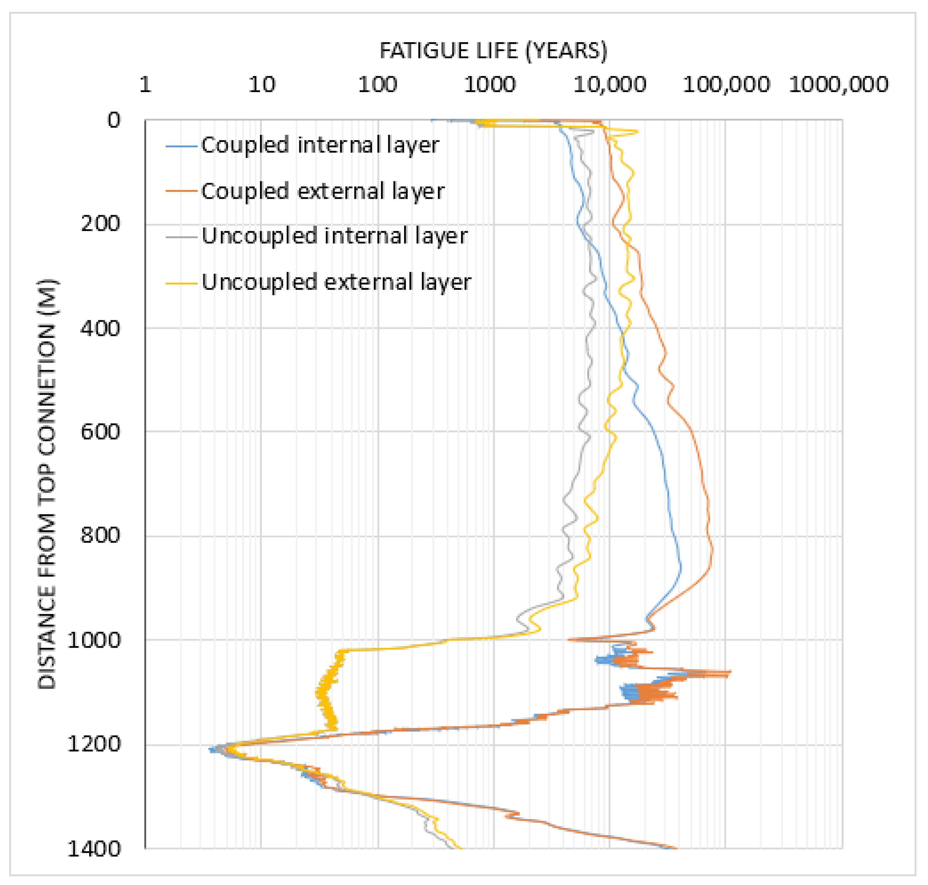
These results bring a new look at fatigue life calculation for such practical applications with asymmetric behavior. They show that the distribution of fatigue life along the riser section may influence the failure sequence of the tensile armors. The risers’ asymmetric distribution may reduce or increase fatigue life compared to symmetric situations and redistribute the fatigue damage on the tensile armors. In the internal tensile armor layers, as shown in the case study, coupled analyses may even present lower fatigue life when compared to the uncoupled results.

Besides the increased accuracy, another advantage of the proposed methodology is the reduction of computing time requirements, which can be 90% lower for irregular analyses than the coupled methodology. In summary, the “coupled RAO” methodology shares the high accuracy provided by the coupled methodology, with considerably lower computational costs for situations with many loading cases.

Finally, it is essential to note that this study builds upon global and local numerical models that have been verified in prior works, thus ensuring the robustness required for their application in the practical design of flexible pipes. Nevertheless, the authors acknowledge the necessity of validating the entire fatigue approach, which can only be accomplished through expensive experimental tests or in-field measurements that are presently unavailable. Consequently, further investigations are needed to thoroughly assess the accuracy of the proposed methodology.

References

1. Pré-Sal Bacia de Santos. Available online: https://comunicabaciadesantos.petrobras.com.br/pre-sal-bacia-de-santos (accessed on 2 December 2023).
2. Offshore Magazine. Harsh Environments, Riser Arrays Drive Turret Design Evolution. Available online: https://www.offshore-mag.com/production/article/16763772/harsh-environments-riser-arrays-drive-turret-design-evolution (accessed on 21 July 2022).
3. API. API RP 17B: Recommended Practice for Flexible Pipe, 5th ed.; American Petroleum Institute: Washington, DC, USA, 2014. [Google Scholar]
4. De Sousa, J.R.M.; de Sousa, F.J.M.; de Siqueira, M.Q.; Sagrilo, L.V.S.; de Lemos, C.A.D. A Theoretical Approach to Predict the Fatigue Life of Flexible Pipes. J. Appl. Math. 2012, 2012, 29. [Google Scholar] [CrossRef]
5. Tagliari, M.d.R.; Antunes, M.R.; Santos, J.G.N.d.; Santos, F.P.d.; Santos, J.M.C.d.; Falcade, T. Tensile Armor Wires Submitted to Slow Strain Rate Tests in a Corrosive Environment and Cathodic Protection: A Comparison Between Two Different Microstructures. Mater. Res. 2019, 22, 1–11. [Google Scholar] [CrossRef]
6. De Motte, R.; Joshi, G.R.; Chehuan, T.; Legent, R.; Kittel, J.; Desamais, N. CO2-SCC in Flexible Pipe Carbon Steel Armour Wires. Corrosion 2022, 78, 547–562. [Google Scholar] [CrossRef] [PubMed]
7. Feret, J.J.; Bournazel, C.L.; Rigaud, J. Evaluation of Flexible Pipes’ Life Expectancy under Dynamic Conditions. In Proceedings of the Offshore Technology Conference, Houston, TX, USA, 5 May 1986. [Google Scholar] [CrossRef]
8. Macfarlane, C.J. Flexible Riser Pipes—Problems and Unknowns. Eng. Struct. 1989, 11, 281–289. [Google Scholar] [CrossRef]
9. Out, J.M.M. On the Prediction of the Endurance Strength of Flexible Pipe. In Proceedings of the Offshore Technology Conference, Houston, TX, USA, 1–4 May 1989. [Google Scholar] [CrossRef]
10. API. API SP 17J: Specification for Unbonded Flexible Pipe, 4th ed.; American Petroleum Institute: Washington, DC, USA, 2014. [Google Scholar]
11. DNV. DNV-OS-F201: Dynamic Risers, 2021-08 ed.; Det Norsk Veritas: Oslo, Norway, 2021. [Google Scholar]
12. Ormberg, H.; Larsen, K. Coupled analysis of floater motion and mooring dynamics for a turret-moored ship. Appl. Ocean. Res. 1998, 20, 55–67. [Google Scholar] [CrossRef]
13. Paulling, J.R. A consistent, large-amplitude analysis of the coupled response of a TLP and tendon system. In Proceedings of the Fifth International Symposium on Offshore Mechanics and Arctic Engineering, Tokyo, Japan, 13–18 April 1986; pp. 126–133. [Google Scholar]
14. Cruces-Giron, A.R.; Mendez Rodriguez, W.S.; Correa, F.N.; Jacob, B.P. An Enhanced Semi-Coupled Methodology for the Analysis and Design of Floating Production Systems. J. Offshore Mech. Arct. Eng. 2021, 143, 041703. [Google Scholar] [CrossRef]
15. Diezel, A.R.; Correa, F.N.; Vaz, M.A.; Jacob, B.P. Investigation of roll damping effects on deep water FPSOs with riser balcony through global coupled analysis. Ships Offshore Struct. 2023, 18, 34–41. [Google Scholar] [CrossRef]
16. Jacob, B.; Bahiense, R.; Correa, F.; Jacovazzo, B. Parallel implementations of coupled formulations for the analysis of floating production systems, part I: Coupling formulations. Ocean. Eng. 2012, 55, 206–218. [Google Scholar] [CrossRef]
17. Larsen, C.M.; Saevik, S.; Qvist, J. Design Analysis. In Handbook on Design and Operation of Flexible Pipes; Fergestad, D., Lotveit, S.A., Eds.; NTNU/4Subsea/MARINTEK: Trondheim, Norway, 2017; Part B. [Google Scholar]
18. Chakrabarti, S.K. Handbook of Offshore Engineering—Volume I; Elsevier: Amsterdam, The Netherlands, 2005. [Google Scholar]
19. Chakrabarti, S.K. Handbook of Offshore Engineering—Volume II; Elsevier: Amsterdam, The Netherlands, 2005. [Google Scholar]
20. Lee, C.H. WAMIT Theory Manual: MIT Report 95-2; Department of Ocean Engineering, Massachusetts Institute of Technology: Cambridge, MA, USA, 1995. [Google Scholar]
21. Journée, J.M.J.; Massie, W.W. Offshore Hydromechanics, 1st ed.; Delft University of Technology: Delft, The Netherlands, 2001. [Google Scholar]
22. Ormberg, H.; Sodahl, N.; Steinkjer, O. Efficient analysis of mooring systems using de-coupled and coupled analysis. In Proceedings of the OMAE98—17th International Conference on Offshore Mechanics and Arctic Engineering, Lisboa, Portugal, 5–9 July 1998. [Google Scholar]
23. Connaire, A.; Kavanagh, K.; Ahilan, R.V.; Goodwin, P. Integrated Mooring & Riser Design: Analysis Methodology. In Proceedings of the Offshore Technology Conference, Houston, TX, USA, 3 May 1999. [Google Scholar]
24. Meirovitch, L. Methods of Analytical Dynamics; McGraw-Hill Book Company: New York, NY, USA, 1970. [Google Scholar]
25. Bathe, K.J. Finite Element Procedures; Prentice-Hall: Upper Saddle River, NJ, USA, 1996. [Google Scholar]
26. Chakrabarti, S.K. Hydrodynamics of Offshore Structures; Computational Mechanics Publications: Boston, MA, USA, 1987. [Google Scholar]
27. Morison, J.R.; O’Brien, M.P.; Johnson, J.W. The Force Exerted by Surface Waves on Piles. Petrol. Trans. 1950, 2, 149–154. [Google Scholar] [CrossRef]
28. Newmark, N.M. A method of computation for structural dynamics. J. Engng Mech Div. ASCE 1959, 85, 67–94. [Google Scholar] [CrossRef]
29. Wood, W.L.; Bossak, M.; Zienkiewicz, O.C. An alpha modification of Newmark’s method. Int. J. Numer. Methods Eng. 1980, 15, 1562–1566. [Google Scholar] [CrossRef]
30. Jacob, B.P.; Ebecken, N.F.F. An optimized implementation of the Newmark/Newton-Raphson algorithm for the time integration of non-linear problems. Commun. Numer. Methods Eng. 1994, 10, 983–992. [Google Scholar] [CrossRef]
31. Yu, J.; Wang, F.; Yu, Y.; Li, H.; Liu, X.; Sun, R. Study on Fatigue Spectrum Analysis and Reliability Analysis of Multilayer Flexible Riser. J. Mar. Sci. Eng. 2022, 10, 1561. [Google Scholar] [CrossRef]
32. Matsuishi, M.; Endo, T. Fatigue of metals subjected to varying stress. Jpn. Soc. Mech. Eng. 1968, 68, 37–40. [Google Scholar]
33. de Sousa, J.R.M.; Magluta, C.; Roitman, N.; Londoño, T.V.; Campello, G.C. A Study on the Response of a Flexible Pipe to Combined Axisymmetric Loads. In Proceedings of the ASME 2013 32nd International Conference on Ocean, Offshore and Arctic Engineering, 11384, Nantes, France, 9–14 June 2013. [Google Scholar]
34. Estrier, P. Updated Method for the Determination of the Service Life of Flexible Risers. In Proceedings of the First European Conference on Flexible Pipes, Umbilicals and Marine Cables (MARINFLEX), London, UK, 10–11 November 1992. [Google Scholar]
35. Saevik, S. Theoretical and Experimental Studies of Stresses in Flexible Pipes. Comput. Struct. 2011, 89, 2273–2291. [Google Scholar] [CrossRef]
36. Wen, Z.; Li, Y.; Wang, H.; Peng, Y. Data-driven spatiotemporal modeling for structural dynamics on irregular domains by stochastic dependency neural estimation. Comput. Methods Appl. Mech. Eng. 2023, 404, 115831. [Google Scholar] [CrossRef]
37. Yuan, L.; Ni, Y.-Q.; Deng, X.-Y.; Hao, S. A-PINN: Auxiliary physics informed neural networks for forward and inverse problems of nonlinear integro-differential equations. J. Comput. Phys. 2022, 462, 111260. [Google Scholar] [CrossRef]
38. Xu, L.; Hu, P.; Li, Y.; Qiu, N.; Chen, G.; Liu, X. Improved Fatigue Reliability Analysis of Deepwater Risers Based on RSM and DBN. J. Mar. Sci. Eng. 2023, 11, 688. [Google Scholar] [CrossRef]
Figure 1. Schematic configuration of a free-hanging riser.
Mathematics 12 01231 g001
Figure 2. Section of a flexible riser showing its layers. Based on [4,5].
Mathematics 12 01231 g002
Figure 3. Wave spectra based on [21].
Mathematics 12 01231 g003
Figure 4. Schematic representation of the hysteretic response of flexible pipes under bending.
Mathematics 12 01231 g004
Figure 5. Tensile armor wires in a cross-section of a flexible pipe.
Mathematics 12 01231 g005
Figure 6. (a) Global wave directions for RAO analysis, (b) Riser balcony and riser position.
Mathematics 12 01231 g006
Figure 7. Flowchart of uncoupled and coupled methodology.
Mathematics 12 01231 g007
Figure 8. 3D global model on SITUA-PROSIM software [16].
Mathematics 12 01231 g008
Figure 9. (a) Situation 01—wave from portside, and (b) Situation 02—wave from starboard.
Mathematics 12 01231 g009
Figure 10. Line coupling effects for (a) heave RAO, stern, and bow waves, and (b) roll RAO, portside, and starboard waves.
Mathematics 12 01231 g010
Figure 11. Riser top connection motion—transverse wave direction (a) portside, (b) starboard; longitudinal wave directions (c) from the stern, (d) from the bow.
Mathematics 12 01231 g011
Figure 12. Acceleration on riser top [m/s2], modulus—transversal waves: (a) portside; (b) starboard.
Mathematics 12 01231 g012
Figure 13. Riser tension amplitude—South direction: (a) top region; (b) TDZ region.
Mathematics 12 01231 g013
Figure 14. Riser tension amplitude histogram (all directions): (a) top region; (b) TDZ region.
Mathematics 12 01231 g014
Figure 15. Riser bending histogram (all directions): (a) top region; (b) TDZ region.
Mathematics 12 01231 g015
Figure 16. Fatigue life distribution along the line.
Mathematics 12 01231 g016
Figure 17. Damage distribution on critical section, top connection (a) internal layer (b) external layer.
Mathematics 12 01231 g017
Figure 18. Damage distribution on critical section, TDZ (a) internal layer (b) external layer.
Mathematics 12 01231 g018