
Synergistic Impacts of Built-Up Characteristics and Background Climate on Urban Vegetation Phenology: Evidence from Beijing, China


1
Centre for Climate–Resilient and Low–Carbon Cities, School of Architecture and Urban Planning, Key Laboratory of New Technology for Construction of Cities in Mountain Area, Ministry of Education, Chongqing University, Chongqing 400045, China
2
Institute for Smart City of Chongqing University in Liyang, Chongqing University, Liyang 213300, China
3
CMA Key Open Laboratory of Transforming Climate Resources to Economy, Chongqing 401147, China
*
Author to whom correspondence should be addressed.
Forests 2024, 15(4), 728; https://doi.org/10.3390/f15040728
Submission received: 5 March 2024
/
Revised: 18 April 2024
/
Accepted: 19 April 2024
/
Published: 21 April 2024
(This article belongs to the Topic Climate Change and Environmental Sustainability, 3rd Volume)
Abstract
:Vegetation is an important strategy for mitigating heat island effects, owed to its shading and evaporative cooling functions. However, urbanization has significantly affected regional vegetation phenology and can potentially weaken the cooling potential of vegetation. Previous studies have mainly focused on national and regional vegetation phenology, but local-scale vegetation phenology and dynamic variations in built-up areas remain unclear. Therefore, this study characterized the vegetation phenology in the densely built-up area of Beijing, China over the period of 2000–2020 based on high-resolution NDVI data using Savitzky–Golay filtering and explored its spatiotemporal characteristics and drivers. The results indicate that the vegetation phenology exhibits significant spatial heterogeneity and clustering characteristics. Compared with vegetation in peripheral blocks, vegetation in central urban blocks generally has an earlier start in the growing season (SOS), later end in the growing season (EOS), and a longer growing season length (GSL). However, the overall distribution of these parameters has experienced a process of decentralization along with urbanization. In terms of drivers, vegetation phenology indicators are mainly influenced by background climate. Specifically, SOS and GSL are mainly affected by temperature (TEP), whereas EOS is mainly influenced by annual precipitation (PRE). Additionally, local environmental factors, particularly the percentage of water body (WAP), also have an impact. Notably, the local environment and background climate have a synergistic effect on vegetation phenology, which is greater than their individual effects. Overall, this study extends the current knowledge on the response of vegetation phenology to urbanization by investigating long-term vegetation phenology dynamics in dense urban areas and provides new insights into the complex interactions between vegetation phenology and built environments.
1. Introduction
Urbanization is an inevitable trend for thriving [1], but it poses great challenges to regional ecological, social, and economic sustainability [2]. A typical process involves replacing natural surfaces with artificial ones, which reduces the latent heat flux in built-up areas and increases the sensible heat flux, thereby inducing the urban heat island (UHI) effect and having profound impacts on regional thermal environments [3]. The global warming and heatwave events also deteriorate the urban thermal environments, having significant impacts on local livelihoods. In addition, urban warming can affect ecosystem processes, especially vegetation phenology [4,5,6,7]. In particular, vegetation phenology (e.g., germination, leaf development, fruiting), as a key representative of the life cycle and seasonal activities of organisms in ecosystems, has been significantly affected by the changes in thermal environments [8]. Owing to its intuitive and sensitive response to microclimatic changes, vegetation phenology is often used to examine and assess the impact of urbanization on ecosystem structure and function and to reflect the complex interactions between regional climate and habitats [9,10].
The development of remote-sensing technology has provided fundamental data for mapping and monitoring vegetation phenology in complex urban areas. Remote-sensing-monitoring methods determine phenological indicators based on time-series vegetation parameters generated by remote-sensing inversion, in contrast with traditional direct observations of phenology on the ground [11,12,13]. Its characteristics of continuous spatial coverage and periodic observations are conducive to understanding the phenology of natural ecosystems from a broader spatiotemporal perspective [14,15]. Accordingly, remote-sensing monitoring is now one of the main technological approaches to investigate the vegetation phenology response to urbanization and has been widely used in relevant research. In particular, the vegetation parameters and land cover conditions inverted by Landsat allow the study of vegetation phenological heterogeneity and urbanization responses at local scales [16,17].
Urban vegetation phenology studies have been widely carried out with the support of remote-sensing data, especially in developing countries with rapid urbanization, to explore microclimate–urban environmental responses [18,19,20]. Most existing studies focus on macro-scale city areas and are usually based on urban–rural dichotomies or urban–rural gradients to explore the characteristics of vegetation phenology [21,22,23]. In these studies, however, the built-up area was considered roughly as a whole, limiting the knowledge of vegetation phenological heterogeneity at smaller scales. Moreover, urban built-up areas, where high temperatures overlap with high population densities, are at significant risk of heat stress. Therefore, it is necessary to assess vegetation phenology in urban areas, which can provide references to enhance the resilience of ecosystem services against potential climate change impacts and assist in predicting potential risks to public health. Exploring the drivers of vegetation phenology can also help to understand the complex relationship between local climate and urban morphology, which is a prerequisite for mitigation–adaptation strategies [24,25]. Previous studies have focused on exploring the relationships between built-up environmental factors (e.g., impervious surfaces, blue infrastructure, and population) and vegetation phenology [13,19,26]. Furthermore, vegetation growth can be potentially regulated by the background climate (e.g., hydrothermal conditions) and its synergy with local drivers, whereas this has received limited attention [11,27,28,29]. Therefore, it is necessary to combine local environmental and background climatic factors to examine their contributions and synergies to vegetation phenology in dense urban areas.
To address these research gaps, this study aims to characterize the vegetation phenology of densely urbanized areas and explore the impacts of built-up characteristics and background climate, with the core area of Beijing selected as the case study area. In general, the core area of Beijing, which is one of the most urbanized and human-disturbed areas in the world, is a suitable case study area. This study analyzed vegetation phenology characteristics of urban built-up areas in detail using multi-source data, such as NDVI, land cover, and meteorology, over the period of 2000–2020. The main objectives of this study are as follows: (1) to examine the temporal trends and spatial patterns of regional vegetation phenology using long-term and high-resolution vegetation indicators; and (2) to explore the driving factors of regional vegetation phenology by integrating local environmental and background climatic factors. The findings of this study are expected to offer insights into environmental health monitoring, urban planning, and climate change assessment, thereby contributing to sustainable urban development and effective management of ecosystem services.
2. Materials and Methods
2.1. Study Area
Beijing (39°28′ N–41°05′ N, 115°25′ E–117°30′ E) is in the northern part of the North China Plain. Its topography tends to be high in the northwest and low in the southeast [30], its average annual temperature is between 10–12 °C, and annual precipitation is 644 mm [31]. In 2020, Beijing had a resident population of 21.893 million, an urbanization level of 87.5%, and a gross domestic product (GDP) of USD 521.099 billion. The internal area of the Fifth Ring Expressway in Beijing was selected as the case study area (Figure 1A), which covers an area of 667 km2, accounting for 4.06% of the area of Beijing’s administrative division. The study area has a total resident population of 9.71 million, accounting for 45% of the whole city population, with a regional average population density of 14,558 people/km2 (2017). Overall, this area is now a crowded and high-density urban area after a long period of development and construction (Figure 1C). Moreover, the thermal environment of the study area is deteriorating due to high-intensity surface construction and anthropogenic heat emission, which can inversely affect the area’s vegetation phenology [32,33,34]. Since blocks are often the basic unit to characterize surface characteristics and energy use, this study divided the study area into 2027 blocks based on the distribution of road networks (Figure 1B) to better explore the regional heterogeneity of vegetation phenology [35,36].
2.2. Data and Materials
2.2.1. Vegetation Index Data
The Normalized Difference Vegetation Index (NDVI) was adopted to extract vegetation phenology indicators. The NDVI is the most widely used vegetation index and provides important information about the greenness and growth status of vegetation by measuring its reflection of infrared and visible light [11,37]. The NDVI was obtained from the Multiscale Satellite Remote Sensing Normalized Difference Vegetation Index product (MUSES NDVI, https://zenodo.org/records/7063344 (accessed 1 December 2023)). The product utilizes the Vegetation Index and Reflectance Data Reconstruction (VIRR) algorithm to process Landsat surface reflectance data and produce an accurate, temporally continuous, and spatially complete NDVI with a temporal resolution of 16 days and a spatial resolution of 30 m [38,39]. In this study, the data were preprocessed through image registration, clipping, and reprojection.
2.2.2. Driving Factor Data
Nine variables were selected as potential factors influencing vegetation phenology. The variables can be grouped into two categories: local environmental factors and background climatic factors (Table 1). The percentage of impervious surface (ISP) and percentage of water body (WAP) were calculated based on the China Annual Land Cover Dataset (CLCD, https://zenodo.org/records/8176941 (accessed 1 December 2023)). The data have a spatial resolution of 30 m and show good consistency in timing [40]. Population density (PD) was calculated based on the 100 m resolution population raster data from the WorldPOP Program (http://www.worldpop.org.uk/ (accessed 1 December 2023)). These data are commonly used in surveys and studies related to population due to their long time series, high accuracy, and high spatial resolution characteristics [41,42]. The Digital Elevation Model (DEM), derived from the Shuttle Radar Topography Mission (SRTM) and with a spatial resolution of 90 m, was used to reflect the block elevation information. Mean temperature (TEP), annual precipitation (PRE), relative humidity (HUM), and hours of daylight (DH) were obtained from the National Meteorological Science Data Center of China Meteorological Administration.
2.3. Analytical Methods
2.3.1. Extraction of Vegetation Phenology Indicators
This study focused on three vegetation phenology indicators: start of the growing season (SOS), end of the growing season (EOS), and length of the growing season (GSL). Vegetation phenology indicator extraction was based on preprocessed NDVI data using the Savitzky–Golay filtering and amplitude method. This method utilized a local polynomial least squares formula to smooth NDVI time-series data, enabling the identification of subtle changes in the processing time series, as well as suppressing noise from clouds and atmospheric disturbances [54,55]. SOS and EOS were identified as the dates when the NDVI first and last crossed the phase NDVI amplitude thresholds, respectively. GSL was set as the time interval between the SOS date and the EOS date (Figure 2). According to previous studies, this threshold was set at 15% [18,33,56].
Considering the complexity of urban subsurface, this study excluded vegetation phenology outliers using land cover data and reference phenology ranges [33]. Moreover, the regional vegetation phenology results extracted from the study could not be validated against field observations because of missing ground station observations, definitional differences, etc. However, the reliability and accuracy of the method were verified in previous studies with the comparisons with field observations [57,58,59]. Figure 3 presents the SOS, EOS, and GSL information of the study area in 2020.
2.3.2. Analysis of Vegetation Phenological Characteristics
Spatial autocorrelation analysis was used to assess the spatial distribution characteristics of vegetation phenology indicators. The Moran’s I is the most commonly used metric for this analysis, with the value ranging between −1 and +1. A higher positive value indicates a higher spatial autocorrelation, meaning that properties of spatially distributed neighboring things have similar trends or values. Conversely, it represents spatial neighborhood properties with opposite trends or values [60]. This method comprises both global and local Moran’s I values, to reflect the spatial autocorrelation for the overall study area and individual spatial units, respectively.
Time-series analysis models (Mann–Kendall test and Sen slope estimator) were used to examine the temporal characteristics of vegetation phenology indicators for each block over the period of 2000–2020. Compared to traditional parametric tests, this model does not require any assumptions regarding the variables. Moreover, it has a wide range of detection and a high level of quantification, making it widely used in the temporal analysis of climate and environmental variables [61].
2.3.3. Analysis of Vegetation Phenology Drivers
This study integrates Spearman correlation coefficients and the Geodetector Model (GDM) to measure the contribution and interaction of local environmental features and background climatic factors on vegetation phenology. The Spearman correlation coefficient is a non-parametric parameter that does not require a specific data distribution, making it more widely applicable than the Pearson correlation coefficient. In this study, it was used to determine the contribution direction (+/−) of factors to the vegetation phenology indicators. GDM is a robust statistical method for exploring the geographic factors of spatial divergence and revealing underlying drivers. Compared to traditional linear regression models, GDM does not only detect the relative contribution of factors, but also assesses the strength, direction, and relationship form (linear or nonlinear) of the interaction between two factors [62]. Furthermore, there is no need to address the issue of multicollinearity among factors during data analysis [63]. The factor detection module and interaction detection module of the model were selected for analysis. The factor detection module was used to measure the explanatory power of the independent variables relative to the dependent variable, which was calculated using the following formula.
where h = 1, 2, …, L, L is the number of factor classifications, and each factor is categorized into five classes in this study based on the natural discontinuity method; Nh and N represent the number of units in class h and the entire region, respectively; and σh2 and σ2 represent the variance in class h and the entire region, respectively. The interaction detection module was used to measure the strength of the interaction and its type, consisting of five types, such as nonlinear weaken, one-factor nonlinear weaken (uni-weaken), two-factor enhance (bi-enhance), and nonlinear enhance and independent.
3. Results
3.1. Spatiotemporal Characteristics of Vegetation Phenology
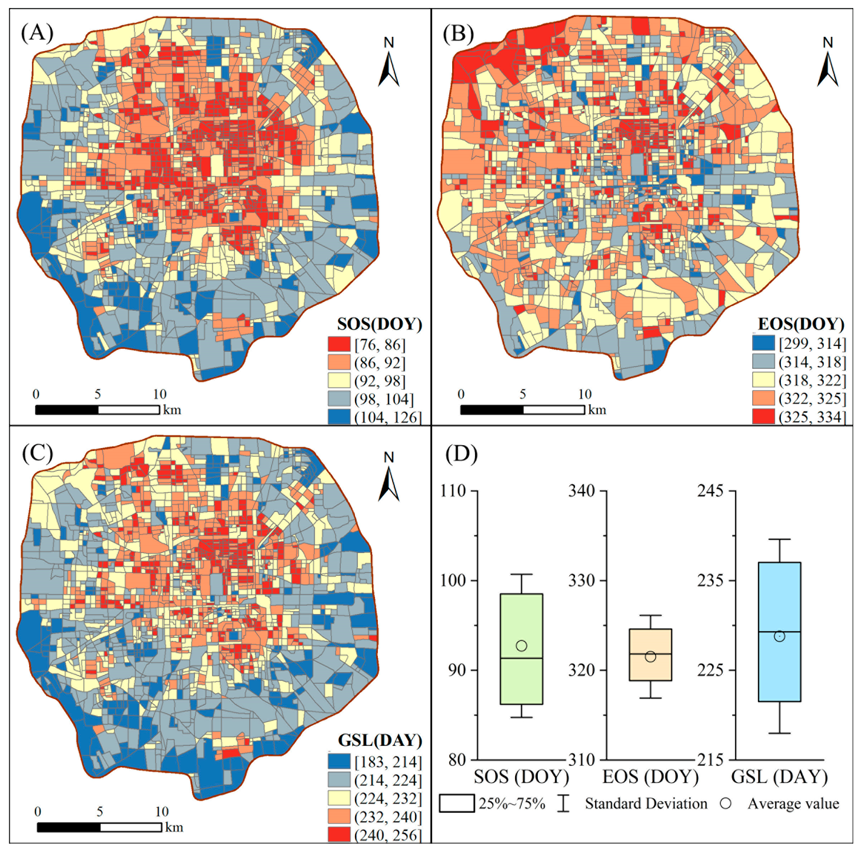
The spatial heterogeneity of vegetation phenology was observed in the core area of Beijing, as shown in Figure 4. The mean values of SOS for 2000–2020 ranged from the 76th to the 126th day, EOS from the 299th to the 334th day, and GSL from 183 to 256 days. To better illustrate the block distribution of vegetation phenology, this study employed the natural discontinuity grading method (Jenks) to rank the vegetation phenology indicators (Figure 4). Spatially, the earlier SOS blocks were predominantly located in the center of the study area, with a gradual postponement from the center to the perimeter. In contrast, the later EOS blocks were mainly located in the regional center and the northwest. Overall, the central blocks had longer GSL than the surrounding blocks. Furthermore, the numerical statistics of phenology indicated that the regional dispersion of SOS was greater than that of EOS, meaning that the fluctuation of SOS between different blocks was greater than EOS (Figure 4D).
The spatial autocorrelation analysis verified the spatial heterogeneity of vegetation phenology (Figure 5A). The regional vegetation phenology indicators showed generally significant positive spatial correlations (Moran’s I > 0, p < 0.05). At the 95% statistical confidence level, there was a significant prevalence of low–low clustering for block SOS (i.e., blocks and their neighboring blocks had smaller values than the overall regional level) compared to other significant autocorrelation types. Conversely, EOS and GSL exhibited a higher prevalence of high–high clustering (i.e., blocks and their neighboring blocks had larger values than the overall regional level). Global Moran’s I showed an overall decrease over the period 2000–2020. The distribution of SOS low–low agglomeration blocks, as well as EOS and GSL high–high agglomeration blocks, were dispersed from the center throughout the region (Figure A1, Figure A2 and Figure A3).
On temporal variation, the blocks and overall trends in vegetation phenology indicators during the period of 2000–2020 are shown in Figure 6. For the SOS, 89% of the blocks showed earlier trends, 54% of which were significant and concentrated in the northern blocks of the region. Meanwhile, 81% of the blocks exhibited trends toward later EOS, with 42% of these trends being significant and spatially dispersed. Most of the blocks demonstrated lengthening GSL trends (89%), with 61% of these blocks showing significant lengthening, particularly in the northern part of the region. Overall, the regional SOS showed a significantly earlier trend (S = −0.75, p < 0.01), the EOS showed a significantly later trend (S = 0.21, p < 0.05), and the GSL showed a significantly longer trend (S = 0.93, p < 0.01) (Figure 6D).
3.2. Drivers and Interactions to Vegetation Phenology
Table 2 and Figure 7 show the direction and strength of the contribution of local built-up factors and background climatic factors to vegetation phenology indicators. Overall, the indicators explained 69.85% (SOS), 52% (EOS), and 64.69% (GSL) of the vegetation phenology indicators in the study area. For SOS, the most important local built-up and background climatic factors controlling its variation were WAP (−9.48%) and TEP (−12.84%), respectively (Figure 7A). Unlike the SOS, the two primary factors affecting the EOS were WAP (+5.28%) and PRE (+17.7%), both of which showed positive delayed effects (Figure 7B). Furthermore, the two primary factors for GSL were WAP (+11.8%) and TEP (+11.71%), both of which contributed to GSL lengthening (Figure 7C). In general, both local built-up factors and background climatic factors play important roles in regulating vegetation phenology, especially for SOS and GSL.
Figure 8 displays the results of interaction strength and type between paired drivers to vegetation phenology. The synergy types of the selected factors were mainly nonlinear enhancement and two-factor enhancement (Bi-enhancement). This implies that pairs of factors acting together contribute more to vegetation phenology than individual effects. The contribution of intragroup interactions related to background climatic factors was higher than that of the two-aspect intergroup interactions and intragroup interactions related to local built-up factors. Among these, the interaction of PRE with other background climatic factors made a prominent contribution to SOS, EOS, and GSL variations. Moreover, inter-group interactions differed among vegetation phenology indicators. TEP and WAP interactions had a greater effect on SOS (Figure 8A). EOS was more affected by PRE and WAP interactions (Figure 8B), and GSL was more affected by TEP and WAP interactions (Figure 8C).
4. Discussion
4.1. Differences of Vegetation Phenology in Densely Built-Up Areas
Overall, the vegetation phenology exhibited spatial and temporal heterogeneity in the core area of Beijing. Spatially, there was earlier SOS, later EOS, and longer GSL in the central region, compared with the surrounding area. In terms of temporal trends, the vegetation phenology growth season generally experienced significant lengthening in 2000–2020 as the region developed (Figure 1C). These results are consistent with those in previous studies based on the urban–rural gradient or urban–rural dichotomy [22,23,33]. Regarding the reasons for this, first, the higher temperatures and longer period of favorable temperatures in built-up areas allow plants to start growing earlier [11]. Second, the increased convection triggered by urbanization results in greater precipitation, providing essential moisture replenishment to vegetation. This has a significant impact on phenology, particularly EOS [20,64]. Third, phenology is subject to the influence of artificial interventions. On the one hand, the necessity for greening has led to the cultivation of more hardy and drought-tolerant plants, which tend to have a longer growing period [65]. On the other hand, the advancement of the SOS and the postponement of the EOS have benefited from careful manual management. With urbanization, this change will continue.
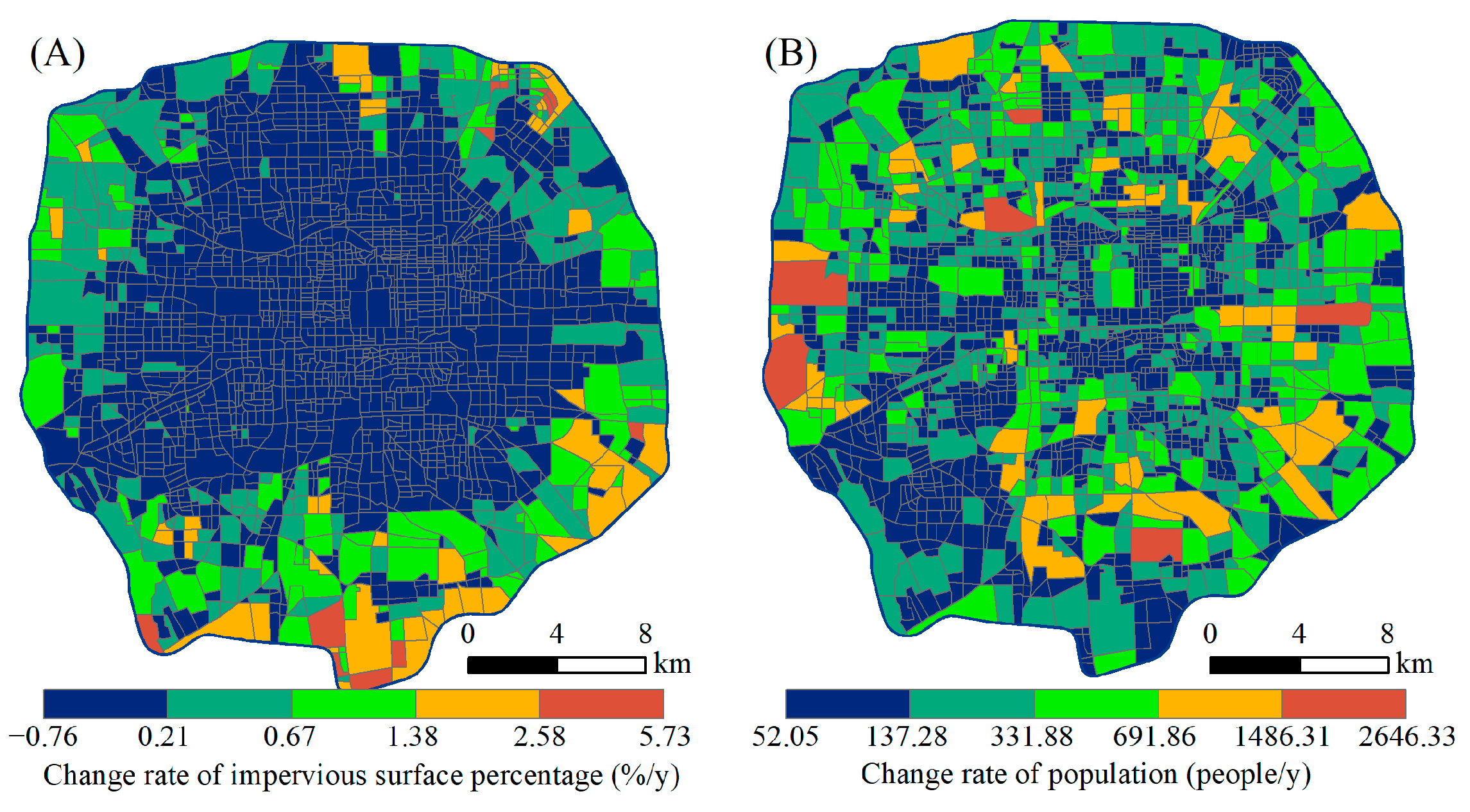
Moreover, there were some differences in the trends and magnitudes of vegetation phenology variation among the blocks. Due to diverse land cover types and different human activity intensities within the region (Figure 1C and Figure A4), microclimatic and environmental conditions vary from one block to another [66,67,68]. This could significantly affect the vegetation growth process, resulting in the significant spatial and temporal differences (i.e., flowering, fruiting) among different blocks. On the one hand, the early development of the regional center and the high intensity of anthropogenic disturbance drove changes in vegetation phenology, resulting in “basins” (low–low clustering) of SOS values and “highlands” (high–high clustering) of EOS and GSL values. Similarly, the peripheral areas, which were underdeveloped in the early stages and had fewer anthropogenic disturbances, showed opposite characteristics of vegetation phenology to the central areas. With regional development, the population in the central urban areas saturated and slowed down, leading to a stabilization of vegetation phenology, while the peripheral areas (especially in the northern part of the region) with ongoing population continued to influence vegetation phenology (Figure A4). On the other hand, the central blocks had undergone “patchy” urban renewal during the development process, increasing the heterogeneity of the vegetation [69]. In contrast, the peripheral areas formed relatively homogeneous built-up environments during the process of rapid development. As a result of these processes, vegetation phenology indicators in the core area of Beijing have evolved from a central distribution to a regionally dispersed distribution.
4.2. Built-Up Environment-Driven Vegetation Phenology under Climate Change
Variations in vegetation phenology often result from a combination of background climatic conditions and local built-up factors. It is crucial to understand the interrelationships between these factors in predicting ecological responses and climate change adaptation. In this study, a robust relationship between background climatic conditions (including temperature, humidity, precipitation, and insolation) and vegetation phenology was also demonstrated in small-scale regions, and the relative contribution was higher than that of local built-up factors. This reflects the persistent effects of long-term climatic trends on plant phenology. Long-term climate changes, such as global warming, lead to changes in temperature, precipitation, and so on, which consequently affect plant ecosystems in a variety of ways, from evapotranspiration to nutrient uptake and photosynthesis [70,71].
Local built-up factors were also important, especially for characterizing the vegetation phenological heterogeneity at small scales. The impact of urbanization on vegetation phenology and its spatial variability could be attributed to many confounding local built-up factors. Previous studies have demonstrated that urbanization-induced subsurface changes could be an important influence on microclimate, leading to different responses of vegetation [72,73]. The significant associations between impervious surfaces, and water bodies with vegetation phenology in this study validated this conclusion. Impervious surfaces (e.g., areas covered by concrete, asphalt, and buildings) can absorb and store more energy, which can result in areas meeting the temperature requirements for vegetation to begin growing sooner [74,75]. Furthermore, local built-up factors, such as population density (affecting anthropogenic heat emissions), topographical features (affecting solar radiation), and the distribution of water bodies (affecting water supply), are also closely related to vegetation phenology [76,77]. It is worth noting that the interactive contribution of background climatic and local built-up factors is much greater than the effect of any single factor on vegetation phenology. This interaction emphasizes the significance of considering various aspects and scales when comprehending plant phenological changes in conjunction with climate variability and urbanization factors [8]. Thus, a deeper understanding of plant adaptations to climate and built-up environments can be achieved.
4.3. Limitations and Future Studies
The study had several limitations. First, this study treats the regional vegetation as uniform, whereas there are often differences in the characteristics of the vegetation itself, such as vegetation structure, physiological status, and species differences, which can lead to different patterns of phenological indicators, thus introducing uncertainty [78]. Second, it is necessary to select more representative and detailed climate and built-up indicators for analysis. This includes climate extreme events, hydrological conditions, artificial management, carbon dioxide concentration, soil, etc., to further improve the factor system for a more comprehensive understanding of the mechanisms. Finally, the use of remote-sensing data introduces computational uncertainty when deriving vegetation phenology indicators due to differences in data sources, pixel mixing, and other issues (e.g., spatial and temporal resolution, and product processing) [79].
This study investigated vegetation phenology and its drivers in built-up areas, providing quantitative evidence of the response of vegetation phenology to high-density built-up environments. In future studies, it is important to combine ground-based observations with remote-sensing monitoring to overcome key challenges, such as collaborative meteorological monitoring and temporal resolution refinement. Furthermore, there is a need to apply the research framework to more cities and synthesize a more comprehensive set of background conditions to explore differences in phenological response patterns and mechanisms. It is essential to promote research of assessing the health of urban ecosystems and optimizing urban planning and management to improve the ecological resilience of cities, promote sustainable urban development, and provide a more pleasant and healthy living environment for residents.
5. Conclusions
This study examined the spatiotemporal characteristics of vegetation phenology and its response to the local built-up and background climatic factors in the core area of Beijing over the period of 2000–2020. The vegetation phenology showed significant spatial heterogeneity. Compared to the surrounding blocks, the blocks in the central area showed earlier SOS, later EOS, and longer GSL. However, the development process has undergone a shift in clustering (low–low cluster for SOS, high–high cluster for EOS, and GSL) from a central to a regionally dispersed distribution. Temporally, there were differences in the magnitude and significance of vegetation phenology between blocks. Moreover, the study area experienced a prior in SOS, a delay in EOS, and an elongation in GSL. The local built-up and background climatic factors had a significant influence on the vegetation phenology variation. The local environmental and background climatic factors that drove the vegetation lifecycle varied and were WAP and TEP for SOS, WAP and PRE for EOS, and WAP and TEP for GSL, respectively. Furthermore, the contribution of two-factor interactions was generally greater than that of single-factor effects. Interactions within groups of background climatic factors had a higher contribution than interactions between groups of local built-up environment-background climate, and interactions within groups of local built-up factors, sequentially. Overall, this study presents the characteristics of vegetation phenology and its drivers in long-time-series high-density built-up areas, which can help to expand the current research scope in this field. This study confirms that climate change and urbanization-related factors drive regional vegetation ecological dynamics. The spatiotemporal heterogeneity results also facilitate the development of more precise urban planning and management strategies to make full use of the ecological services they provide in each region.
Author Contributions
X.F.: Conceptualization, Data curation, Formal analysis, Investigation, Methodology, and Writing—original draft; B.-J.H.: Conceptualization, Funding acquisition, Methodology, Project administration, Supervision, and Writing—review and editing. All authors have read and agreed to the published version of the manuscript.
Funding
This project is supported by the National Natural Science Foundation of China (No: 42301339), the Fundamental Research Funds for the Central Universities (Grant No. 2023CDJXY-008), and CMA Key Open Laboratory of Transforming Climate Resources to Economy (No. 2023018).
Data Availability Statement
The data presented in this study are available on request from the corresponding author.
Conflicts of Interest
The authors declare no conflicts of interest.
Appendix A
Figure A1.
SOS local autocorrelation results for the study area in 2000–2020.

Figure A2.
EOS local autocorrelation results for the study area in 2000–2020.

Figure A3.
GSL local autocorrelation results for the study area in 2000–2020.

Figure A4.
Trends in the percentage of impervious surface and population in study area blocks in 2000–2020. ((A) Change rate of impervious surface percentage; (B) Change rate of population).
Figure A4.
Trends in the percentage of impervious surface and population in study area blocks in 2000–2020. ((A) Change rate of impervious surface percentage; (B) Change rate of population).

References
- Lu, Y.H.; Song, W.; Lyu, Q.Q. Assessing the effects of the new-type urbanization policy on rural settlement evolution using a multi-agent model. Habitat Int. 2022, 127, 14. [Google Scholar] [CrossRef]
- He, B.J. Cause-related injustice, process-related injustice, effect-related injustice and regional heat action planning priorities: An empirical study in Yangtze River Delta and Chengdu-Chongqing urban agglomerations. Landsc. Urban Plan. 2023, 237, 104800. [Google Scholar] [CrossRef]
- Wei, F.L.; Li, S.C.; Liu, D.H.; Liang, Z.; Wang, Y.X.; Wang, H.; Wang, Y.Y.; Zhang, Y.J.; Liu, Y.L. Analysis of the driving factors of precipitation change during the development of the Jing-Jin-Ji urban agglomeration. Urban Clim. 2023, 51, 20. [Google Scholar] [CrossRef]
- Singh, M.; Sharston, R. Normalized urban heat island (UHI) indicators: Classifying the temporal variation of UHI for building energy simulation (BES) applications. Build. Simul. 2023, 16, 1645–1658. [Google Scholar] [CrossRef]
- Huang, W.T.K.; Masselot, P.; Bou-Zeid, E.; Fatichi, S.; Paschalis, A.; Sun, T.; Gasparrini, A.; Manoli, G. Economic valuation of temperature-related mortality attributed to urban heat islands in European cities. Nat. Commun. 2023, 14, 12. [Google Scholar] [CrossRef]
- Ren, J.L.; Shi, K.Z.; Kong, X.F.; Zhou, H.Z. On-site measurement and numerical simulation study on characteristic of urban heat island in a multi-block region in Beijing, China. Sust. Cities Soc. 2023, 95, 18. [Google Scholar] [CrossRef]
- Fukano, Y.; Yamori, W.; Misu, H.; Sato, M.P.; Shirasawa, K.; Tachiki, Y.; Uchida, K. From green to red: Urban heat stress drives leaf color evolution. Sci. Adv. 2023, 9, 3542. [Google Scholar] [CrossRef] [PubMed]
- Li, D.J.; Barve, N.; Brenskelle, L.; Earl, K.; Barve, V.; Belitz, M.W.; Doby, J.; Hantak, M.M.; Oswald, J.A.; Stucky, B.J.; et al. Climate, urbanization, and species traits interactively drive flowering duration. Glob. Chang. Biol. 2021, 27, 892–903. [Google Scholar] [CrossRef] [PubMed]
- Zhang, J.; Hao, F.; Wu, Z.; Li, M.; Zhang, X.; Fu, Y. Response of vegetation phenology to extreme climate and its mechanism. Acta Geogr. Sin. 2023, 78, 2241–2255. [Google Scholar] [CrossRef]
- Wang, S.X.; Wu, Z.F.; Gong, Y.F.; Wang, S.B.; Zhang, W.; Zhang, S.S.; De Boeck, H.J.; Fu, Y.S.H. Climate warming shifts the time interval between flowering and leaf unfolding depending on the warming period. Sci. China Life Sci. 2022, 65, 2316–2324. [Google Scholar] [CrossRef] [PubMed]
- Piao, S.L.; Liu, Q.; Chen, A.P.; Janssens, I.A.; Fu, Y.S.; Dai, J.H.; Liu, L.L.; Lian, X.; Shen, M.G.; Zhu, X.L. Plant phenology and global climate change: Current progresses and challenges. Glob. Chang. Biol. 2019, 25, 1922–1940. [Google Scholar] [CrossRef] [PubMed]
- Wu, C.Y.; Peng, J.; Ciais, P.; Peñuelas, J.; Wang, H.J.; Beguería, S.; Black, T.A.; Jassal, R.S.; Zhang, X.Y.; Yuan, W.P.; et al. Increased drought effects on the phenology of autumn leaf senescence. Nat. Clim. Chang. 2022, 12, 943–949. [Google Scholar] [CrossRef]
- Li, X.C.; Zhou, Y.Y.; Asrar, G.R.; Mao, J.F.; Li, X.M.; Li, W.Y. Response of vegetation phenology to urbanization in the conterminous United States. Glob. Chang. Biol. 2017, 23, 2818–2830. [Google Scholar] [CrossRef] [PubMed]
- Heijmans, M.M.; Magnússon, R.; Lara, M.J.; Frost, G.V.; Myers-Smith, I.H.; van Huissteden, J.; Jorgenson, M.T.; Fedorov, A.N.; Epstein, H.E.; Lawrence, D.M. Tundra vegetation change and impacts on permafrost. Nat. Rev. Earth Environ. Int. 2022, 3, 68–84. [Google Scholar] [CrossRef]
- Zhao, C.H.; Weng, Q.H.; Wang, Y.G.; Hu, Z.M.; Wu, C.Y. Use of local climate zones to assess the spatiotemporal variations of urban vegetation phenology in Austin, Texas, USA. GISci. Remote Sens. 2022, 59, 393–409. [Google Scholar] [CrossRef]
- Li, L.Z.; Li, X.C.; Asrar, G.; Zhou, Y.Y.; Chen, M.; Zeng, Y.L.; Li, X.J.; Li, F.; Luo, M.; Sapkota, A.; et al. Detection and attribution of long-term and fine-scale changes in spring phenology over urban areas: A case study in New York State. Int. J. Appl. Earth Obs. Geoinf. 2022, 110, 10. [Google Scholar] [CrossRef]
- Li, X.C.; Zhou, Y.Y.; Meng, L.; Asrar, G.R.; Lu, C.Q.; Wu, Q.S. A dataset of 30 m annual vegetation phenology indicators (1985–2015) in urban areas of the conterminous United States. Earth Syst. Sci. Data 2019, 11, 881–894. [Google Scholar] [CrossRef]
- Hu, M.C.; Li, X.J.; Xu, Y.X.; Huang, Z.H.; Chen, C.; Chen, J.J.; Du, H.Q. Remote sensing monitoring of the spatiotemporal dynamics of urban forest phenology and its response to climate and urbanization. Urban Clim. 2024, 53, 101810. [Google Scholar] [CrossRef]
- Ding, H.Y.; Xu, L.M.; Elmore, A.J.; Shi, Y.L. Vegetation Phenology Influenced by Rapid Urbanization of The Yangtze Delta Region. Remote Sens. 2020, 12, 18. [Google Scholar] [CrossRef]
- Jochner, S.; Menzel, A. Urban phenological studies—Past, present, future. Environ. Pollut. 2015, 203, 250–261. [Google Scholar] [CrossRef] [PubMed]
- Jia, W.X.; Zhao, S.Q.; Zhang, X.Y.; Liu, S.G.; Henebry, G.M.; Liu, L.L. Urbanization imprint on land surface phenology: The urban-rural gradient analysis for Chinese cities. Glob. Chang. Biol. 2021, 27, 2895–2904. [Google Scholar] [CrossRef] [PubMed]
- Liu, Z.H.; Zhou, Y.; Feng, Z.T. Response of vegetation phenology to urbanization in urban agglomeration areas: A dynamic urban-rural gradient perspective. Sci. Total Environ. 2022, 864, 161109. [Google Scholar] [CrossRef] [PubMed]
- Yang, J.; Luo, X.; Jin, C.; Xiao, X.M.; Xia, J.H. Spatiotemporal patterns of vegetation phenology along the urban–rural gradient in Coastal Dalian, China. Urban For. Urban Green. 2020, 54, 126784. [Google Scholar] [CrossRef]
- He, B.J.; Ding, L.; Prasad, D. Relationships among local-scale urban morphology, urban ventilation, urban heat island and outdoor thermal comfort under sea breeze influence. Sust. Cities Soc. 2020, 60, 102289. [Google Scholar] [CrossRef]
- He, B.J.; Wang, J.; Liu, H.; Ulpiani, G. Localized synergies between heat waves and urban heat islands: Implications on human thermal comfort and urban heat management. Environ. Res. 2021, 193, 110584. [Google Scholar] [CrossRef] [PubMed]
- Li, P.; Sun, M.; Liu, Y.X.; Ren, P.X.; Peng, C.H.; Zhou, X.L.; Tang, J.Y. Response of Vegetation Photosynthetic Phenology to Urbanization in Dongting Lake Basin, China. Remote Sens. 2021, 13, 17. [Google Scholar] [CrossRef]
- Zhang, J.; Chen, S.Z.; Wu, Z.F.; Fu, Y.H. Review of vegetation phenology trends in China in a changing climate. Prog. Phys. Geogr. 2022, 46, 829–845. [Google Scholar] [CrossRef]
- Wei, J.; Xu, F.; Cole, E.F.; Sheldon, B.C.; de Boer, W.F.; Wielstra, B.; Fu, H.H.; Gong, P.; Si, Y.L. Spatially heterogeneous shifts in vegetation phenology induced by climate change threaten the integrity of the avian migration network. Glob. Chang. Biol. 2024, 30, e17148. [Google Scholar] [CrossRef] [PubMed]
- Chen, S.Z.; Fu, Y.S.; Hao, F.H.; Li, X.Y.; Zhou, S.; Liu, C.M.; Tang, J. Vegetation phenology and its ecohydrological implications from individual to global scales. Geogr. Sustain. 2022, 3, 334–338. [Google Scholar] [CrossRef]
- Zhang, Z.Y.; Xu, X.D.; Qiao, L.; Gong, D.Y.; Kim, S.J.; Wang, Y.J.; Mao, R. Numerical simulations of the effects of regional topography on haze pollution in Beijing. Sci. Rep. 2018, 8, 5504. [Google Scholar] [CrossRef] [PubMed]
- Overview of Beijing. Available online: http://www.weather.com.cn/cityintro/101010100.shtml (accessed on 11 April 2024).
- Fu, X.C.; Yao, L.; Xu, W.T.; Wang, Y.X.; Sun, S. Exploring the multitemporal surface urban heat island effect and its driving relation in the Beijing-Tianjin-Hebei urban agglomeration. Appl. Geogr. 2022, 144, 102714. [Google Scholar] [CrossRef]
- Zhang, Y.H.; Yin, P.Y.; Li, X.C.; Niu, Q.D.; Wang, Y.X.; Cao, W.T.; Huang, J.X.; Chen, H.; Yao, X.C.; Yu, L.; et al. The divergent response of vegetation phenology to urbanization: A case study of Beijing city, China. Sci. Total Environ. 2022, 803, 150079. [Google Scholar] [CrossRef] [PubMed]
- Siddique, M.A.; Wang, Y.; Xu, N.H.; Ullah, N.; Zeng, P. The Spatiotemporal Implications of Urbanization for Urban Heat Islands in Beijing: A Predictive Approach Based on CA-Markov Modeling (2004–2050). Remote Sens. 2021, 13, 20. [Google Scholar] [CrossRef]
- Gao, Y.J.; Zhao, J.Y.; Han, L. Exploring the spatial heterogeneity of urban heat island effect and its relationship to block morphology with the geographically weighted regression model. Sust. Cities Soc. 2022, 76, 103431. [Google Scholar] [CrossRef]
- Chen, X.T.; Wang, Z.T.; Bao, Y.; Luo, Q.Y.; Wei, W.F. Combined impacts of buildings and urban remnant mountains on thermal environment in multi-mountainous city. Sust. Cities Soc. 2022, 87, 104247. [Google Scholar] [CrossRef]
- Xu, Y.; Yang, Y.P.; Chen, X.N.; Liu, Y.X.Y. Bibliometric Analysis of Global NDVI Research Trends from 1985 to 2021. Remote Sens. 2022, 14, 20. [Google Scholar] [CrossRef]
- Xiao, Z.Q.; Liang, S.L.; Wang, T.T.; Liu, Q. Reconstruction of Satellite-Retrieved Land-Surface Reflectance Based on Temporally-Continuous Vegetation Indices. Remote Sens. 2015, 7, 9844–9864. [Google Scholar] [CrossRef]
- Xiao, Z.Q.; Liang, S.L.; Tian, X.D.; Jia, K.; Yao, Y.J.; Jiang, B. Reconstruction of Long-Term Temporally Continuous NDVI and Surface Reflectance From AVHRR Data. IEEE J. Sel. Topics Appl. Earth Observ. Remote Sens. 2017, 10, 5551–5568. [Google Scholar] [CrossRef]
- Yang, J.; Huang, X. The 30 m annual land cover dataset and its dynamics in China from 1990 to 2019. Earth Syst. Sci. Data 2021, 13, 3907–3925. [Google Scholar] [CrossRef]
- Lai, S.J.; Ruktanonchai, N.W.; Zhou, L.C.; Prosper, O.; Luo, W.; Floyd, J.R.; Wesolowski, A.; Santillana, M.; Zhang, C.; Du, X.J.; et al. Effect of non-pharmaceutical interventions to contain COVID-19 in China. Nature 2020, 585, 410–413. [Google Scholar] [CrossRef] [PubMed]
- Gaughan, A.; Stevens, F.; Huang, Z.J.; Nieves, J.; Sorichetta, A.; Lai, S.J.; Ye, X.Y.; Linard, C.; Hornby, G.M.; Hay, S.I.; et al. Spatiotemporal patterns of population in mainland China, 1990 to 2010. Sci. Data 2016, 3, 160005. [Google Scholar] [CrossRef] [PubMed]
- Zhang, L.; Yang, L.; Zohner, C.M.; Crowther, T.W.; Li, M.; Shen, F.; Guo, M.; Qin, J.; Yao, L.; Zhou, C. Direct and indirect impacts of urbanization on vegetation growth across the world’s cities. Sci. Adv. 2022, 8, eabo0095. [Google Scholar] [CrossRef] [PubMed]
- Qiu, T.; Song, C.H.; Zhang, Y.L.; Liu, H.S.; Vose, J.M. Urbanization and climate change jointly shift land surface phenology in the northern mid-latitude large cities. Remote Sens. Environ. 2020, 236, 111477. [Google Scholar] [CrossRef]
- Lian, X.; Piao, S.L.; Li, L.Z.X.; Li, Y.; Huntingford, C.; Ciais, P.; Cescatti, A.; Janssens, I.A.; Penuelas, J.; Buermann, W.; et al. Summer soil drying exacerbated by earlier spring greening of northern vegetation. Sci. Adv. 2020, 6, eaax0255. [Google Scholar] [CrossRef] [PubMed]
- Gu, Z.G.; Zhang, Z.; Yang, J.H.; Wang, L.L. Quantifying the Influences of Driving Factors on Vegetation EVI Changes Using Structural Equation Model: A Case Study in Anhui Province, China. Remote Sens. 2022, 14, 4203. [Google Scholar] [CrossRef]
- Tian, M.Q.; Zhou, J.Z.; Jia, B.J.; Lou, S.J.; Wu, H.L. Impact of Three Gorges Reservoir Water Impoundment on Vegetation-Climate Response Relationship. Remote Sens. 2020, 12, 2860. [Google Scholar] [CrossRef]
- Li, X.J.; Du, H.Q.; Zhou, G.M.; Mao, F.J.; Zhu, D.E.; Zhang, M.; Xu, Y.X.; Zhou, L.; Huang, Z.H. Spatiotemporal patterns of remotely sensed phenology and their response to climate change and topography in subtropical bamboo forests during 2001–2017: A case study in Zhejiang Province, China. GISci. Remote Sens. 2023, 60, 22. [Google Scholar] [CrossRef]
- Zhou, D.C.; Zhao, S.Q.; Liu, S.G.; Zhang, L.X. Spatiotemporal trends of terrestrial vegetation activity along the urban development intensity gradient in China’s 32 major cities. Sci. Total Environ. 2014, 488, 136–145. [Google Scholar] [CrossRef] [PubMed]
- Shen, M.G.; Wang, S.P.; Jiang, N.; Sun, J.P.; Cao, R.Y.; Ling, X.F.; Fang, B.; Zhang, L.; Zhang, L.H.; Xu, X.Y.; et al. Plant phenology changes and drivers on the Qinghai-Tibetan Plateau. Nat. Rev. Earth Environ. 2022, 3, 633–651. [Google Scholar] [CrossRef]
- He, X.J.; Chen, S.S.; Wang, J.M.; Smith, N.G.; Rossi, S.; Yang, H.J.; Liu, J.Q.; Chen, L. Delaying effect of humidity on leaf unfolding in Europe. Sci. Total Environ. 2021, 800, 149563. [Google Scholar] [CrossRef] [PubMed]
- Yuan, M.X.; Zhao, L.; Lin, A.W.; Li, Q.J.; She, D.X.; Qu, S. How do climatic and non-climatic factors contribute to the dynamics of vegetation autumn phenology in the Yellow River Basin, China? Ecol. Indic. 2020, 112, 106112. [Google Scholar] [CrossRef]
- Zhu, L.Y.; Sun, S.; Li, Y.; Liu, X.B.; Hu, K. Effects of climate change and anthropogenic activity on the vegetation greening in the Liaohe River Basin of northeastern China. Ecol. Indic. 2023, 148, 110105. [Google Scholar] [CrossRef]
- Liu, J.H.; Zhan, P. The impacts of smoothing methods for time-series remote sensing data on crop phenology extraction. In Proceedings of the 2016 IEEE International Geoscience and Remote Sensing Symposium (IGARSS), Beijing, China, 10–15 July 2016; pp. 2296–2299. [Google Scholar]
- Mirahmadi, A.; Yazdanpanah, H.; Momeni Shahraki, M. Evaluation of smoothing methods for GREENNESS time series reconstruction and phenological estimation from Landsat 8 satellite data. J. Phys. Geogr. Res. 2022, 54, 55–70. [Google Scholar]
- He, Y.; Fan, G.F.; Zhang, X.W.; Li, Z.Q.; Gao, D.W. Vegetation phenological variation and its response to climate changes in Zhejiang province. J. Nat. Resour. 2013, 28, 220–233. [Google Scholar]
- Rodriguez-Galiano, V.F.; Dash, J.; Atkinson, P.M. Intercomparison of satellite sensor land surface phenology and ground phenology in Europe. Geophys. Res. Lett. 2015, 42, 2253–2260. [Google Scholar] [CrossRef]
- Meroni, M.; Rembold, F.; Verstraete, M.; Gommes, R.; Schucknecht, A.; Beye, G. Investigating the Relationship between the Inter-Annual Variability of Satellite-Derived Vegetation Phenology and a Proxy of Biomass Production in the Sahel. Remote Sens. 2014, 6, 5868–5884. [Google Scholar] [CrossRef]
- Vintrou, E.; Bégué, A.; Baron, C.; Saad, A.; Lo Seen, D.; Traoré, S. A Comparative Study on Satellite- and Model-Based Crop Phenology in West Africa. Remote Sens. 2014, 6, 1367–1389. [Google Scholar] [CrossRef]
- Anselin, L. Local indicators of spatial association—LISA. Geogr. Anal. 1995, 27, 93–115. [Google Scholar] [CrossRef]
- Hassan, Q.K.; Ejiagha, I.R.; Ahmed, M.R.; Gupta, A.; Rangelova, E.; Dewan, A. Remote Sensing of Local Warming Trend in Alberta, Canada during 2001–2020, and Its Relationship with Large-Scale Atmospheric Circulations. Remote Sens. 2021, 13, 3441. [Google Scholar] [CrossRef]
- Xu, W.T.; Yao, L.; Fu, X.C.; Wang, Y.X.; Sun, S. Response of PM2.5 variations to changing urbanization process in different climatic backgrounds of China. Urban CLim. 2022, 45, 101273. [Google Scholar] [CrossRef]
- Hu, D.; Meng, Q.Y.; Zhang, L.L.; Zhang, Y. Spatial quantitative analysis of the potential driving factors of land surface temperature in different “Centers” of polycentric cities: A case study in Tianjin, China. Sci. Total Environ. 2020, 706, 135244. [Google Scholar] [CrossRef] [PubMed]
- Ahmed, G.; Zan, M.; Helili, P.; Kasimu, A. Responses of Vegetation Phenology to Urbanisation and Natural Factors along an Urban-Rural Gradient: A Case Study of an Urban Agglomeration on the Northern Slope of the Tianshan Mountains. Land 2023, 12, 1108. [Google Scholar] [CrossRef]
- Díaz, J.G.; Gutiérrez-Bustillo, A.M.; Rojo, J. The phenological response of European vegetation to urbanisation is mediated by macrobioclimatic factors. Sci. Total Environ. 2023, 905, 167092. [Google Scholar] [CrossRef] [PubMed]
- Lin, Z.L.; Xu, H.Q.; Yao, X.; Yang, C.X.; Yang, L.J. Exploring the relationship between thermal environmental factors and land surface temperature of a “furnace city” based on local climate zones. Build. Environ. 2023, 243, 110732. [Google Scholar] [CrossRef]
- Wu, Z.F.; Man, W.; Ren, Y. Influence of tree coverage and micro-topography on the thermal environment within and beyond a green space. Agric. Forest Meteorol. 2022, 316, 108846. [Google Scholar] [CrossRef]
- Kamal, A.; Abidi, S.M.H.; Mahfouz, A.; Kadam, S.; Rahman, A.; Hassan, I.G.; Wang, L.L. Impact of urban morphology on urban microclimate and building energy loads. Energy Build. 2021, 253, 111499. [Google Scholar] [CrossRef]
- Cao, K.X.; Deng, Y.; Wang, W.X.; Liu, S.H. The spatial heterogeneity and dynamics of land redevelopment: Evidence from 287 Chinese cities. Land Use Policy 2023, 132, 106760. [Google Scholar] [CrossRef]
- Higgins, S.I.; Conradi, T.; Muhoko, E. Shifts in vegetation activity of terrestrial ecosystems attributable to climate trends. Nat. Geosci. 2023, 16, 147. [Google Scholar] [CrossRef]
- Yuan, M.X.; Zhao, L.; Lin, A.W.; Wang, L.C.; Li, Q.J.; She, D.X.; Qu, S. Impacts of preseason drought on vegetation spring phenology across the Northeast China Transect. Sci. Total Environ. 2020, 738, 140297. [Google Scholar] [CrossRef] [PubMed]
- Shen, F.X.; Yang, L.; Zhang, L.; Guo, M.; Huang, H.L.; Zhou, C.H. Quantifying the direct effects of long-term dynamic land use intensity on vegetation change and its interacted effects with economic development and climate change in jiangsu, China. J. Environ. Manag. 2023, 325, 116562. [Google Scholar] [CrossRef] [PubMed]
- Rogers, C.A.; Chen, J.M. Land cover and latitude affect vegetation phenology determined from solar induced fluorescence across Ontario, Canada. Int. J. Appl. Earth Obs. Geoinf. 2022, 114, 103036. [Google Scholar] [CrossRef]
- Wu, W.; Li, L.D.; Li, C.L. Seasonal variation in the effects of urban environmental factors on land surface temperature in a winter city. J. Clean. Prod. 2021, 299, 126897. [Google Scholar] [CrossRef]
- Hua, L.Z.; Zhang, X.X.; Nie, Q.; Sun, F.Q.; Tang, L.N. The impacts of the expansion of urban impervious surfaces on urban heat islands in a coastal city in China. Sustainability 2020, 12, 475. [Google Scholar] [CrossRef]
- Raj, S.; Paul, S.K.; Chakraborty, A.; Kuttippurath, J. Anthropogenic forcing exacerbating the urban heat islands in India. J. Environ. Manag. 2020, 257, 110006. [Google Scholar] [CrossRef]
- Sun, R.H.; Wang, Y.N.; Chen, L.D. A distributed model for quantifying temporal-spatial patterns of anthropogenic heat based on energy consumption. J. Clean. Prod. 2018, 170, 601–609. [Google Scholar] [CrossRef]
- Li, X.X.; Liang, E.R.Y.; Camarero, J.J.; Rossi, S.; Zhang, J.T.; Zhu, H.F.; Fu, Y.H.; Sun, J.; Wang, T.; Piao, S.L.; et al. Warming-induced phenological mismatch between trees and shrubs explains high-elevation forest expansion. Nat. Sci. Rev. 2023, 10, nwad182. [Google Scholar] [CrossRef] [PubMed]
- Kabano, P.; Lindley, S.; Harris, A. Evidence of urban heat island impacts on the vegetation growing season length in a tropical city. Landsc. Urban Plan. 2021, 206, 103989. [Google Scholar] [CrossRef]
Figure 1.
Overview of the study area ((A) Topography of Beijing; (B) Regional block division; (C) Regional percentage of impervious surface urbanization and population).
Figure 1.
Overview of the study area ((A) Topography of Beijing; (B) Regional block division; (C) Regional percentage of impervious surface urbanization and population).

Figure 2.
Process of extracting vegetation phenology indicators.

Figure 3.
Status of vegetation phenology indicators in the study area (in 2020). ((A) Start of the growing season (SOS); (B) End of the growing season (EOS); (C) Length of the growing season (GSL)).
Figure 3.
Status of vegetation phenology indicators in the study area (in 2020). ((A) Start of the growing season (SOS); (B) End of the growing season (EOS); (C) Length of the growing season (GSL)).

Figure 4.
Spatial distribution of vegetation phenology indicators in the study area in 2000–2020. ((A) Mean SOS of the blocks; (B) Mean EOS of the blocks; (C) Mean GSL of the blocks; (D) Statistics on vegetation phenology indicators).
Figure 4.
Spatial distribution of vegetation phenology indicators in the study area in 2000–2020. ((A) Mean SOS of the blocks; (B) Mean EOS of the blocks; (C) Mean GSL of the blocks; (D) Statistics on vegetation phenology indicators).

Figure 5.
Spatial autocorrelation of vegetation phenology indicators in the study area in 2000–2020. ((A) Changes in global Moran’s I for vegetation phenology indicators; (B) Percentage of SOS spatial autocorrelation types; (C) Percentage of EOS spatial autocorrelation types; (D) Percentage of GSL spatial autocorrelation types).

Figure 6.
Trend in vegetation phenology indicators in the study area in 2000–2020. ((A) SOS trends in blocks; (B) EOS trends in blocks; (C) GSL trends in blocks; (D) Regional trends and block statistics on vegetation phenology indicators).
Figure 6.
Trend in vegetation phenology indicators in the study area in 2000–2020. ((A) SOS trends in blocks; (B) EOS trends in blocks; (C) GSL trends in blocks; (D) Regional trends and block statistics on vegetation phenology indicators).

Figure 7.
The relative contribution of drivers to vegetation phenology indicators. ((A) Relative contribution of drivers to SOS; (B) Relative contribution of drivers to EOS; (C) Relative contribution of drivers to GSL).
Figure 7.
The relative contribution of drivers to vegetation phenology indicators. ((A) Relative contribution of drivers to SOS; (B) Relative contribution of drivers to EOS; (C) Relative contribution of drivers to GSL).

Figure 8.
Interaction effect between drivers on vegetation phenology. ((A) Driver interactions on SOS; (B) Driver interactions on EOS; (C) Driver interactions on GSL).
Figure 8.
Interaction effect between drivers on vegetation phenology. ((A) Driver interactions on SOS; (B) Driver interactions on EOS; (C) Driver interactions on GSL).


Table 1.
Potential drivers selected for analysis.
| Variable | Category | Description (Units) | Reference |
|---|---|---|---|
| ISP | Local environment | Percentage of impervious surface (%) | [43,44] |
| PD | Local environment | Population density (104 people/km2) | [43,45] |
| WAP | Local environment | Percentage of water body (%) | [46,47] |
| DEM | Local environment | Mean elevation (m) | [46,48] |
| PRE | Background climate | Annual precipitation (mm) | [43,49] |
| TEP | Background climate | Mean temperature (°C) | [43,49] |
| HUM | Background climate | Mean relative humidity (%) | [50,51] |
| DH | Background climate | Hours of daylight (h) | [52,53] |
Table 2.
Spearman’s correlation between vegetation phenology and drivers.
| ISP | PD | DEM | WAP | PRE | TEP | HUM | DH | |
|---|---|---|---|---|---|---|---|---|
| SOS | − ** | − ** | − ** | − | − ** | − ** | + ** | − ** |
| EOS | − ** | + ** | + ** | + ** | + ** | − ** | − | + |
| GSL | + ** | + ** | + ** | + ** | + ** | + ** | − ** | + ** |
**: p < 0.05.
Disclaimer/Publisher’s Note: The statements, opinions and data contained in all publications are solely those of the individual author(s) and contributor(s) and not of MDPI and/or the editor(s). MDPI and/or the editor(s) disclaim responsibility for any injury to people or property resulting from any ideas, methods, instructions or products referred to in the content. |
© 2024 by the authors. Licensee MDPI, Basel, Switzerland. This article is an open access article distributed under the terms and conditions of the Creative Commons Attribution (CC BY) license (https://creativecommons.org/licenses/by/4.0/).
Share and Cite
MDPI and ACS Style
Fu, X.; He, B.-J. Synergistic Impacts of Built-Up Characteristics and Background Climate on Urban Vegetation Phenology: Evidence from Beijing, China. Forests 2024, 15, 728. https://doi.org/10.3390/f15040728
AMA Style
Fu X, He B-J. Synergistic Impacts of Built-Up Characteristics and Background Climate on Urban Vegetation Phenology: Evidence from Beijing, China. Forests. 2024; 15(4):728. https://doi.org/10.3390/f15040728
Chicago/Turabian StyleFu, Xuecheng, and Bao-Jie He. 2024. "Synergistic Impacts of Built-Up Characteristics and Background Climate on Urban Vegetation Phenology: Evidence from Beijing, China" Forests 15, no. 4: 728. https://doi.org/10.3390/f15040728
Note that from the first issue of 2016, this journal uses article numbers instead of page numbers. See further details here.