Article

Comparison of Surface Ozone Variability in Mountainous Forest Areas and Lowland Urban Areas in Southeast China

1
Institute of Geography, School of Geographic Science, Fujian Normal University, Fuzhou 350117, China
2
Department of Geography and Planning, University of Toronto, Toronto, ON M5S 3G3, Canada
3
Fujian Key Laboratory of Severe Weather, Fuzhou 350008, China
4
Nanping Meteorological Bureau, Jianyang 354200, China
5
Fujian Academy of Environmental Sciences, Fuzhou 350117, China
6
Xiamen Key Laboratory of Straits Meteorology, Xiamen Meteorological Bureau, Xiamen 361000, China
*
Author to whom correspondence should be addressed.
Atmosphere 2024, 15(5), 519; https://doi.org/10.3390/atmos15050519
Submission received: 6 February 2024 / Revised: 7 April 2024 / Accepted: 18 April 2024 / Published: 24 April 2024
(This article belongs to the Special Issue Characteristics and Source Apportionment of Urban Air Pollution)

Abstract

:
The ozone (O3) variations in southeast China are largely different between mountainous forest areas located inland, and lowland urban areas located near the coast. Here, we selected these two kinds of areas to compare their similarities and differences in surface O3 variability from diurnal to seasonal scales. Our results show that in comparison with the lowland urban areas (coastal areas), the mountainous forest areas (inland areas) are characterized with less human activates, lower precursor emissions, wetter and colder meteorological conditions, and denser vegetation covers. This can lead to lower chemical O3 production and higher O3 deposition rates in the inland areas. The annual mean of 8-h O3 maximum concentrations (MDA8 O3) in the inland areas are ~15 μg·m−3 (i.e. ~15%) lower than that in the coastal areas. The day-to-day variation in surface O3 in the two types of the areas is rather similar, with a correlation coefficient of 0.75 between them, suggesting similar influences on large scales, such as weather patterns, regional O3 transport, and background O3. Over 2016–2020, O3 concentrations in all the areas shows a trend of “rising and then falling”, with a peak in 2017 and 2018. Daily MDA8 O3 correlates with solar radiation most in the coastal areas, while in the inland areas, it is correlated with relative humidity most. Diurnally, during the morning, O3 concentrations in the inland areas increase faster than in the coastal areas in most seasons, mainly due to a faster increase in temperature and decrease in humidity. While in the evening, O3 concentrations decrease faster in the inland areas than in the coastal areas, mostly attributable to a higher titration effect in the inland areas. Seasonally, both areas share a double-peak variation in O3 concentrations, with two peaks in spring and autumn and two valleys in summer and winter. We found that the valley in summer is related to the summer Asian monsoon that induces large-scale convections bringing local O3 upward but blocking inflow of O3 downward, while the one in winter is due to low O3 production. The coastal areas experienced more exceedance days (~30 days per year) than inland areas (~5-10 days per year), with O3 sources largely from the northeast. Overall, the similarities and differences in O3 concentrations between inland and coastal areas in southeastern China are rather unique, reflecting the collective impact of geographic-related meteorology, O3 precursor emissions, and vegetation on surface O3 concentrations.

1. Introduction

Ozone (O3) in the surface layer, or surface O3, is a major pollutant which is generated through photochemical reactions involving volatile organic compounds (VOCs) and nitrogen oxides (NOx) in the presence of solar radiation [1,2,3]. Excessive O3 concentrations can have significant implications for human health and vegetation growth [4,5,6,7]. In recent decades, a noticeable increase trend in surface O3 concentrations in China has been observed [8,9,10,11,12]. As of 2019, O3 accounts for 41.8% of the total days exceeding the air quality standard in China [13,14]. The increasing trends are strong in clustered megacity areas, such as in the Beijing-Tianjin-Hebei region (BTH), the Yangtze River Delta (YRD), the Pearl River Delta (PRD), and the Sichuan Basin [15,16].
Surface O3 variability in a region depends on chemistry, transport, and deposition processes in that region. Environmental factors and their interactions modulate surface O3 variability in different time scales through their influences on the three processes. O3 precursor emissions and meteorological are regarded as the major environmental factors, as well as the most studied ones. Another important environmental factor is vegetation cover, especially for densely vegetated areas.
Fujian province, situated along the southeastern coast of China, experiences unique surface O3 variability compared to the rest of China. Having lower O3 precursor emissions, the O3 level in Fujian is lower than in the BTH, YRD, and PRD areas. In the meantime, Fujian has not been immune from O3 pollution in recent years. Surface O3 concentrations in some areas in the province increased over 2015–2020, with a range of 0.3~4.6 μg·m−3 yr−1, similar to that in YRD and PRD [17]. There are large contrasts in surface O3 variability across the province, especially between the inland mountainous areas and coastal urban areas, resulting from large differences in O3 precursor emissions, meteorological conditions, and vegetation covers, which are due to different economic developments, topography, and proximity to the coastline. The Mt. Wuyi area is located in the northwestern Fujian with plenty of forest covers. The Mt. Wuyi National Park is an UNESCO world heritage site with limited human activities. Although there has been a growing number of studies on O3 in the province recently [17,18,19,20,21,22,23,24,25], our understanding of surface O3 variability in the remote and mountainous forest areas and comparisons with other regions are still limited. Here, we collect O3 observations in two mountainous forest areas in Wuyishan and Nanping near the Mt. Wuyi and two urban areas in lowlands: Fuzhou and Putian. Based on the geographic locations, we name Wuyishan and Nanping as inland areas and Fuzhou and Putian as coastal areas. We examine the similarities and differences in surface O3 variability from diurnal to seasonal scales between the two types of areas, especially between Wuyishan and other areas. We explore underlying mechanisms driving these similarities and differences using data analysis, chemical transport simulations, and trajectory simulations. Such enhanced understanding can inform strategies for the management and control of surface O3 in the areas.
This paper is organized as follows. In Section 2, we introduce the study areas, data, and methods used in this study. The results are discussed in Section 3 in seven subsections. Section 3.1 compares differences in environmental factors between the inland and coastal areas; Section 3.2 shows daily time series of O3 concentrations over 2016–2021. Based on this, impacts of environmental factors on surface O3 variability are discussed in Section 3.3 and Section 3.4, which shed some light on the diurnal variation and seasonal variations to be discussed in Section 3.5 and Section 3.6. O3 exceedance days and associated source regions are examined in Section 3.7. Finally, conclusions are provided in Section 4.

2. Study Area, Data, and Methods

2.1. Study Area

Fujian province is located along the coast in southeast China (Figure 1). With a forest cover of 66.8% and low industrial emissions, Fujian is one of the most environmentally clean regions in the country. The topography of the province is mainly mountainous and hilly, with high terrain in the northwest and low terrain in the southeast. For our study goals, we selected observational stations in Wuyishan (WYS), which is 40 km away from Mt. Wuyi National Park, and a close-by Nanping (NP) to present mountainous forest areas. In comparison, stations in Fuzhou (FZ) and Putian (PT) in similar latitudes (25–28° N, 117–118° E) of a subtropical region are selected to represent urban areas in lowlands. The longitude, latitude, and elevation of the observational stations are showed in Figure 1 and listed in Table 1. The environmental monitoring stations in Fuzhou and Putian are with altitudes of 10~18 m, while the stations in inland areas reside at higher altitudes of about 106~223 m (Figure 1 and Table 1).

2.2. Data

2.2.1. Air Quality, Emission, and Leaf Area Data

Ground-based air quality data were collected from two sources. The hourly pollutant concentrations in Wuyishan from 2016 to 2020 were from the Wuyishan City Bureau of Ecology and Environment, while the hourly pollutant data for the other stations were from the National Environmental Monitoring General Station of China (http://www.cnemc.cn/, accessed on 5 September 2023). The air quality observations are strictly quality-controlled and released with a 1 h temporal resolution. The mean O3 and NO2, for Fuzhou, Putian, Nanping, and Wuyishan were determined by averaging observations in all available stations in each of the areas (Figure 1, Table 1). The pollutant concentrations refer to the Technical Provisions on Ambient Air Quality Index (HJ633-2012) and National Ambient Air Quality Standards (GB3095-2012) [18,26]. The daily maximum 8 h average (MDA8) O3 concentrations represent the highest daily O3 levels. An exceedance day is defined as the day with MDA8 O3 concentrations larger than 160 μg m−3. The emissions data were obtained from the Multi-resolution Emission Inventory for China (MEIC) emission inventory of Tsinghua University (http://meicmodel.org.cn/, accessed on 10 January 2024), and leaf area index (LAI) data were obtained from GLASS data from the University of Maryland (http://glass.umd.edu/, accessed on 5 July 2023).

2.2.2. Meteorological Observations and Reanalysis Data

Meteorological data, including hourly surface air temperature, relative humidity (RH), wind speed, and precipitation from 2016 to 2020, were from the Fujian Meteorological Bureau. The locations of meteorological stations in each area are listed in Table 1. The saturated water vapor pressure difference (VPD) data were calculated from RH and air temperature data. Downward solar radiation to the surface (R), RH at 850 hPa, daily mean boundary layer height (BLH), horizontal U, V winds at 850 hPa (U850,V850), and vertical velocity at 850 hPa (W850) were from the ERA5 reanalysis of the European Weather Prediction Centre (https://cds.climate.copernicus.eu/, accessed on 15 May 2023), which has a temporal resolution of 1 h and a spatial resolution of 0.25° × 0.25°. The EAR5 dataset has been verified in previous studies [27,28]. The daily mean of meteorological data is taken from the period of 01:00–24:00 China Standard Time (Local standard time, LST), while the daily total precipitation data are taken from the same period. BLH and R are taken from the mean during the period of 08:00–20:00 LST. The operational radiosonde observations over southern China during are collected (https://www.ncei.noaa.gov/products/weather-balloon/integratedglobal-radiosonde-archive, accessed on 5 March 2024). The data are used to calculate monthly mean convective available potential energy (CAPE) in Fujian, so as to examine the mean seasonality of convection in the study areas.

2.3. Methods

2.3.1. Statistical Analysis

To explore the relationship between meteorological factors and O3, we quantified the correlation between each meteorological factor and MDA8 O3 using the Pearson correlation coefficient (r), as shown in Equation (1).
r = i = 1 n ( X i Y i ) i = 1 n ( X i X ¯ ) 2 i = 1 n ( Y i Y ¯ ) 2
where X is meteorological factor, Y is O3 concentrations, n is the number of samples, and i is an index for counting the sample.

2.3.2. Random Forest Model

The Random Forest (RF) is a supervised machine-learning algorithm based on decision trees proposed by Breiman [29]. Each of its trees is modeled using a subset of the training data, so it provides approximations of different models and then makes predictions by averaging the predicted values of each model [30]. The results of the RF are not easily overfitted and are more stable than those of a single decision tree [31]. It is worth noting that the relationship between meteorological factors and O3 concentrations is often complex, interactive, and nonlinear. RF is a robust machine-learning technique that can effectively capture the nonlinear relationship between independent and dependent variables and it is widely used in the study of air quality [32,33,34].
To investigate the correlation between meteorological factors and MDA8 O3 concentrations, we chose input meteorological factors, including local factors (radiation, RH, Tmax, precipitation, wind speed, and BLH), and large circulation-related factors (U850, V850, and W850). We built an RF model with n_estimator and max_depth set to 1500 and 20, respectively. We used 80% of the MDA8 O3 data as the training dataset, while the remaining 20% was reserved for the testing purpose. The model was then evaluated using the test dataset, and the output displays the importance of each meteorological factor in predicting MDA8 O3 concentrations.

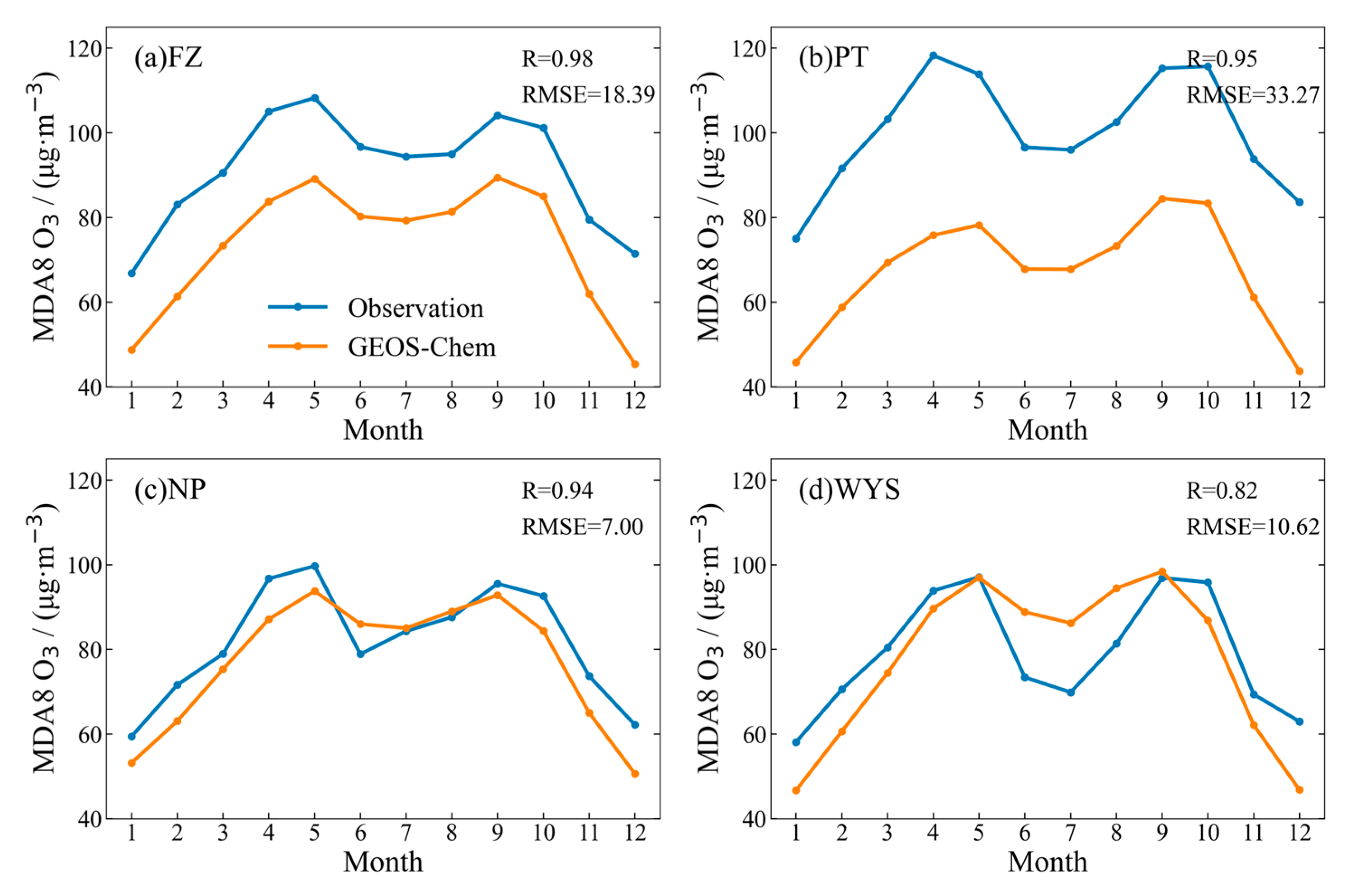
2.3.3. GEOS-Chem Model

GEOS-Chem is a global 3-D model of atmospheric chemistry driven by meteorological input from the Goddard Earth Observing System (GEOS) of the NASA Global Modeling and Assimilation Office [35]. It is used by research groups around the world to investigate a wide range of atmospheric environmental issues.
We conducted a nested full chemistry simulation using GEOS-Chem (v12.9.3; http://geos-chem.org, accessed on 15 February 2023). The horizontal resolution over eastern China is 0.5° × 0.625°, with boundary conditions archived every 3 h from global simulations with 2° × 2.5° resolution. Emissions are based on the Harvard–NASA Emission Component (HEMCO) [36]. Biogenic VOC emissions, including isoprene, monoterpenes, and sesquiterpenes, are from the Model of Emissions of Gases and Aerosols from Nature (MEGAN v2.1) [37]. Soil NOx emissions are based on the available nitrogen (N) in soils and edaphic conditions such as soil temperature and moisture [38]. Global anthropogenic emissions are from the Community Emissions Data System (CEDS) [39]. Vegetation fire emissions are from the Global Fire Emissions Database (GFED4). In this simulation, processes of chemistry, transport, and deposition can be output directly [40].
In addition, a tagged-O3 simulation was made to further examine O3 transport from different sources. In the tagged-O3 simulation, the horizontal resolution is 2.0° × 2.5° in latitude and longitude. Surface O3  ( O 3 T o t a l ) is partitioned into local production ( O 3 L o c a l ), O3 from the rest of China ( O 3 R O C ), from the rest of the world O 3 R O W , and from the stratosphere ( O 3 S t r a t ):
O 3 T o t a l = O 3 L o c a l + O 3 R O C + O 3 R O W + O 3 S t r a t
By examining seasonal variations in the components, along with the associated meteorological conditions, we aim to provide an explanation for the seasonality in surface O3 in Fujian.
Comparison between observed MDA8 O3 and the simulated one based on the nested full chemistry simulation is showed in Figure 2. Generally, GEOS-Chem can reproduce the observed monthly variation in MDA8 O3 with some degrees of biases.

2.3.4. Trajectory Analysis

Trajectory statistical models (TSM) include the potential source contribution function (PSCF) and concentration weighted trajectory (CWT) [41]. The method uses the NOAA HYSPLIT model with the NCEP/NCAR meteorological reanalysis dataset generated from GDAS (http://www.arl.noaa.gov/, accessed on 3 June 2023). One-day backward trajectories with 1 h intervals were simulated from one of the four receptor areas on O3 exceedance days. The arrival level in the model was set as 500 m above ground level and HYSPLIT was run every hour at start times from 00:00 to 23:00 LST.
PSCF is a trajectory-based method combined with O3 concentrations for identifying potential source regions [42,43,44]. The PSCF values reflect the probabilities of pollution trajectories in the area. The study field was divided into 0.5° × 0.5° grid cells. The PSCF is defined in the following equation:
P S C F i j = m i j n i j
where i and j are the cell indexes in latitude and longitude, respectively; nij is the number of endpoints that fall in the ijth cell; mij is the endpoint number in the same cell that corresponds to samples that are higher than the criterion values. The arbitrary weighting function Wij is applied to reduce the uncertainties caused by small values of nij. The function Wij used in this study is defined as follows:
P S C F i j = m i j n i j W i j
W i j = 1.0   3 n a v e < n i j   0.7   1.5 n a v e < n i j 3 n a v e 0.4   n a v e < n i j 1.5 n a v e   0.2   n i j n a v e  
The CWT method weights trajectories based on O3 concentrations, reflecting the pollution levels along the trajectory. The study region was divided into an array of 0.1° × 0.1° grid cells. A CWT is determined with the following equation:
C W T i j = i = 1 M C l t i j l i = 1 M t i j l
W C W T i j = C W T i j · W i j
where CWTij represents the average weighted concentrations of the trajectory l in the ijth grid cell; M is the total number of back trajectories; Cl is the observed O3 concentrations corresponding to trajectory l; tijl is the residence time of trajectory l in the ijth cell.

3. Results and Discussion

3.1. Comparison of O3 Precursors Emissions, Meteorology, and Vegetation Covers between the Inland and Coastal Areas

Figure 3 shows the differences in O3 precursor emission, meteorology, and vegetation cover between the inland and coastal areas, along with information on the economics and elevation. The coastal areas are more economically developed and have a larger population than the inland areas, as GDP is higher in the coastal areas than in the inland areas; the permanent population in Wuyishan is only 240 thousand, in comparison with 2.68 million in Nanping, 3.13 million in Putian, and 8.13 million in Fuzhou. Consequently, O3 precursor emissions are much lower in the inland areas than in the coastal areas, being 89.9 tons (603%), 33.5 tons (596%), and 176.5 tons (837%) lower for VOC, NOx, and CO, respectively. In terms of meteorological conditions (Figure 3h–k), the average annual downward solar radiation, average air temperature, average relative humidity, and wind speed over 2016–2022 were 14.87 W·m−2 (5%), 1.2 °C (6%), 2% (3%), and 0.7 m·s−1 (50%) higher in the coastal areas than in the inland areas. Among the four areas, Putian has the highest average annual solar radiation of 340.43 W·m−2 and temperature of 21.68 °C, while Wuyishan has the highest average annual rainfall of 2039.8 mm. In proximity of Wuyishan National Park, Wuyishan and Nanping have a higher vegetation coverage than Fujian and Putian, showing 0.5 (18.5%) higher LAI (Figure 3g).
In summary, the differences in emissions, meteorological conditions, and vegetation covers would lead to different variations in O3 concentrations between the inland and coastal areas in Fujian to be explored in this study.

3.2. Daily Variability in Surface O3 Concentrations

Figure 4 shows the time series of daily MDA8 O3 concentrations from 2016 to 2020 in Fuzhou, Putian, Nanping, and Wuyishan. The noticeable difference among the areas is that O3 concentrations in the coastal areas are higher than in the inland areas. The annual mean MDA8 O3 concentrations in Wuyishan and Nanping are 79.2 and 81.8 μg·m−3, in comparison with 91.3 and 100.5 μg·m−3 in Fuzhou and Putian, with the mean O3 concentrations of 95.9 μg·m−3 in the coastal areas and 80.5 μg·m−3 in the inland areas. Compared to surface O3 in BTH, YRD, and other regions in eastern China [45], the O3 levels in Fujian are lower.
On the other hand, there are some similarities in daily variation of MDA8 O3 concentrations in the four areas. First, the daily variation in MDA8 O3 concentrations in the four areas is rather similar, with a correlation coefficient of 0.75 in the daily time series between the inland and coastal areas, and 0.85 and 0.77 between the two coastal areas and between the two inland areas. Second, all the areas show a two-peak seasonal variation in O3 concentrations: one in spring and the other in fall (to be discussed in Section 3.6). Third, the interannual variation and trend in O3 concentrations are also similar. Over 2016–2020, O3 concentrations in all the areas shows a trend of “rising and then falling”, with a peak in 2017 and 2018. These similar variations in O3 concentrations in the four areas indicate some influential factors on large scales, such as weather patterns, O3 transport at large scales, and background O3.

3.3. Impact of O3 Precursors and Vegetation Covers on Surface O3 Variability

Generally, regions with higher emissions of VOCs and NOx tend to have higher O3 concentrations and are more susceptible to O3 pollution [46]. Figure 5a shows GEOS-Chem simulated net chemical production varying with season. It is obvious that the net chemical production is highest in Putian, followed by Fuzhou, Nanping, and Wuyishan. This is in the same order of the O3 precursor emissions showed in Figure 3d–f. Hong et al. [22] reported that VOCs are higher in Fuzhou than in Mt. Wuyi region, are higher in summer than in winter. Previous studies also suggested that the difference in the O3 magnitude between the inland and coastal areas in Fujian are generally attributed to lower O3 precursor emissions in the inland areas than in the coastal areas [47]. Such variations in VOCs with season and region lead to high O3 production in summer than in the other seasons (Figure 5a) and in the coastal areas than in the inland areas. Note that the seasonal variation in chemical production appears larger than that in O3 precursor emissions (Figure 3), especially for the coastal areas, suggesting influences of other factors, such as local and regional meteorological conditions, to be discussed in Section 3.4.
In contrast, Figure 5b shows that GEOS-Chem simulated deposition is higher in the inland areas than in the coastal areas, reflecting the difference of foliage amount, in terms of LAI (Figure 3g). Stomatal and non-stomatal deposition can remove surface O3 from the air effectively [48]. As expected, the deposition increases with foliage amount. The seasonal variation in deposition also closely follows that in LAI. Note that seasonal meteorology also plays an important role in modulating deposition through its impact on the stomatal opening. The overall meteorological impact is to be explored in section.

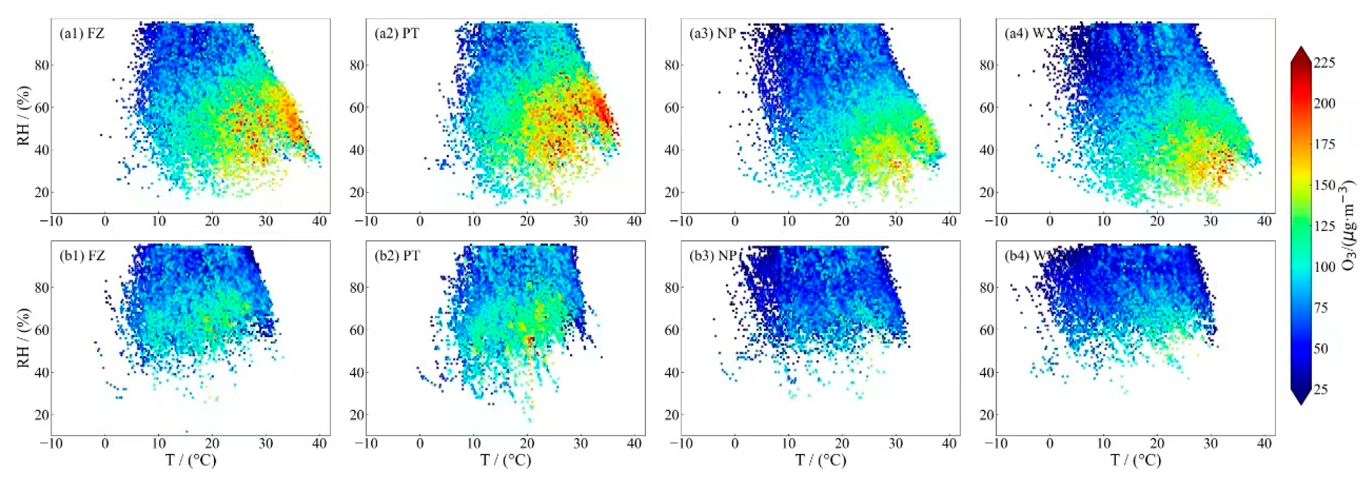
3.4. Impact of Meteorological Conditions on Surface O3 Variability

Although it is known that meteorology can significant impact surface O3 variability, such impacts remain complicated and challenging to assess because meteorology can simultaneously modulate the three processes controlling O3 variability, including chemistry, transport, and deposition. Meteorology at local and regional scales can jointly modulate O3 variability [45],. At the local scale, solar radiation and temperature directly affect O3 chemical generation and lose [49]; humid air generally promotes deposition through reducing leaf stomatal conductance [50]. Overall, local high temperature, low humidity, and low horizontal wind speed are more conducive to O3 pollution [10,51,52]. Meteorological impacts also vary with time scale and region. For instance, in summer, the most important meteorological factor to daily O3 variability is RH in central and southern East China, whereas it is temperature in the northern China [45,53]. In Section 3.4.1 and Section 3.4.2, we focus on local meteorological impacts on surface O3 variability on hourly and daily time scales, respectively.

3.4.1. Meteorological Impact Surface O3 Concentrations on Hourly Scale

The hourly data for temperature, RH, and O3 were divided into daytime (08:00–20:00 LST) and nighttime (20:00–08:00 LST). Because local meteorological variables are correlated, we focused on three important variables: temperature, humidity, and wind direction. Figure 6 shows that high O3 values in all the four areas were associated with high temperature and low humidity during the daytime. Specifically, high O3 concentrations appeared more when the temperature ranged from 20 °C to 40 °C and the humidity ranged from 20% to 60%. The coastal areas experienced higher O3 concentrations and more severe O3 pollution during the day, while the inland areas had fewer high O3 values. At night, O3 depletion dominated, resulting in lower O3 concentrations. Under the same temperature and humidity ranges, Nanping and Wuyishan experienced lower O3 concentrations at both night and daytime than Fuzhou and Putin, reflecting the impact of precursor emissions.
The wind field comprises wind direction and wind speed, which are crucial for the vertical and horizontal transport of O3. Figure 7a–d shows that southeast and northwest winds prevail in Fuzhou, while north and northeast winds prevail in Putian. Wind speeds in Fuzhou and Putian are mostly above 1.5 m/s. In contrast, Nanping and Wuyishan are mainly covered by northeast and north winds, with lower wind speeds. Hourly O3 concentrations in the coastal areas are sensitive to wind directions, with highest O3 concentrations occurring under southeast winds (Figure 7e,f). In contrast, O3 concentrations in the two inland areas are insensitive to wind direction (Figure 7g,h).

3.4.2. Meteorological Impact Surface O3 Concentrations on Daily Scale

When anthropogenic emissions vary little daily, the day-to-day O3 variability depends largely on daily meteorology [51]. Figure 8a displays the correlation between meteorological factors and MDA8 O3 for each area based on observations over 2016–2020. Overall, MDA8 O3 is positively correlated with daily R, maximum temperature (Tmax), and BLH, but negatively correlated with RH, precipitation (Rain), U850, and V850. Overall, R and RH are with highest correlation with daily variation of O3 concentrations in all the areas, as also reported by Lei and Chen [54,55]. The most influential meteorological factors are different between the inland and coast areas. In annual mean, the factor is radiation for the coastal areas but RH for the inland areas. Note that the MDA8 O3 variations are more sensitive to meteorological factors in the inland areas of Nanping and Wuyishan than that in the coastal areas of Fuzhou and Putian. Ji et al. [17] also suggested that meteorological conditions have a greater effect on O3 concentrations in areas with lower levels of anthropogenic emissions.
There are seasonal differences in the correlation coefficient (r) between daily MDA8 O3 concentrations and meteorological factors (Figure 8b–e). O3 concentrations are more sensitive to meteorological conditions in spring, autumn, and winter than in summer. The correlations between MDA8 O3 and the most relevant meteorological factors, such as RH, become weaker in summer (r ranges over −0.50~0.52) than in the other seasons (r ranges over −0.83~0.81).
Relationships between meteorological factors and O3 concentrations can be complex, interactive, and nonlinear. To investigate the joint influence of meteorological factors on MDA8 O3 concentrations, we constructed a model using RF. Based on the discussed correlations, nine meteorological factors were selected as driving forces for the model, including solar radiation, RH, Tmax, BLH, wind speed, and precipitation.
Figure 9 shows a comparison between observed and predicted MDA8 O3 with the RF model for each area. The prediction is better for the inland areas than for coastal areas, with R² descending in the order: Wuyishan (0.68) > Nanping (0.64) > Fuzhou (0.60) > Putian (0.54). This indicates again that the meteorological factors modulate day-to-day variability of MDA8 O3 more in the inland areas than in the coastal areas.
The RF model automatically evaluates the importance of each meteorological element to MDA8 O3. Figure 10 shows that factors such as R, RH, Tmax, V850, and U850 have a significant impact on MDA8 O3 concentrations. The RF analysis confirmed that the meteorological factor that holds the most significance in the coastal areas is R, whereas inland areas place greatest importance on RH. Overall, meteorological conditions have a greater impact on O3 concentrations in inland areas where anthropogenic emissions are lower.

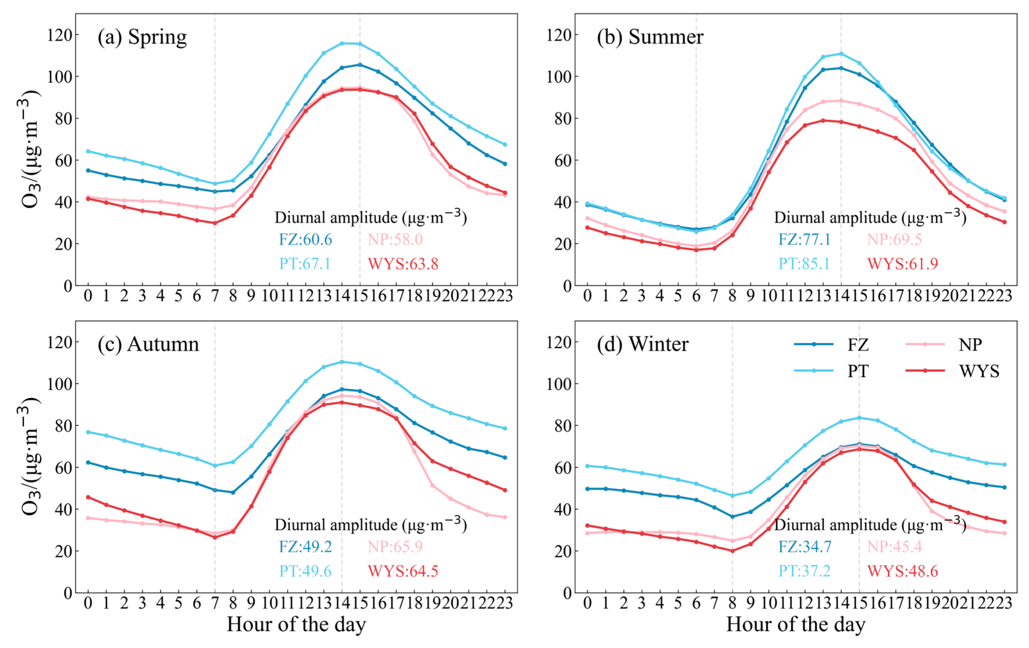
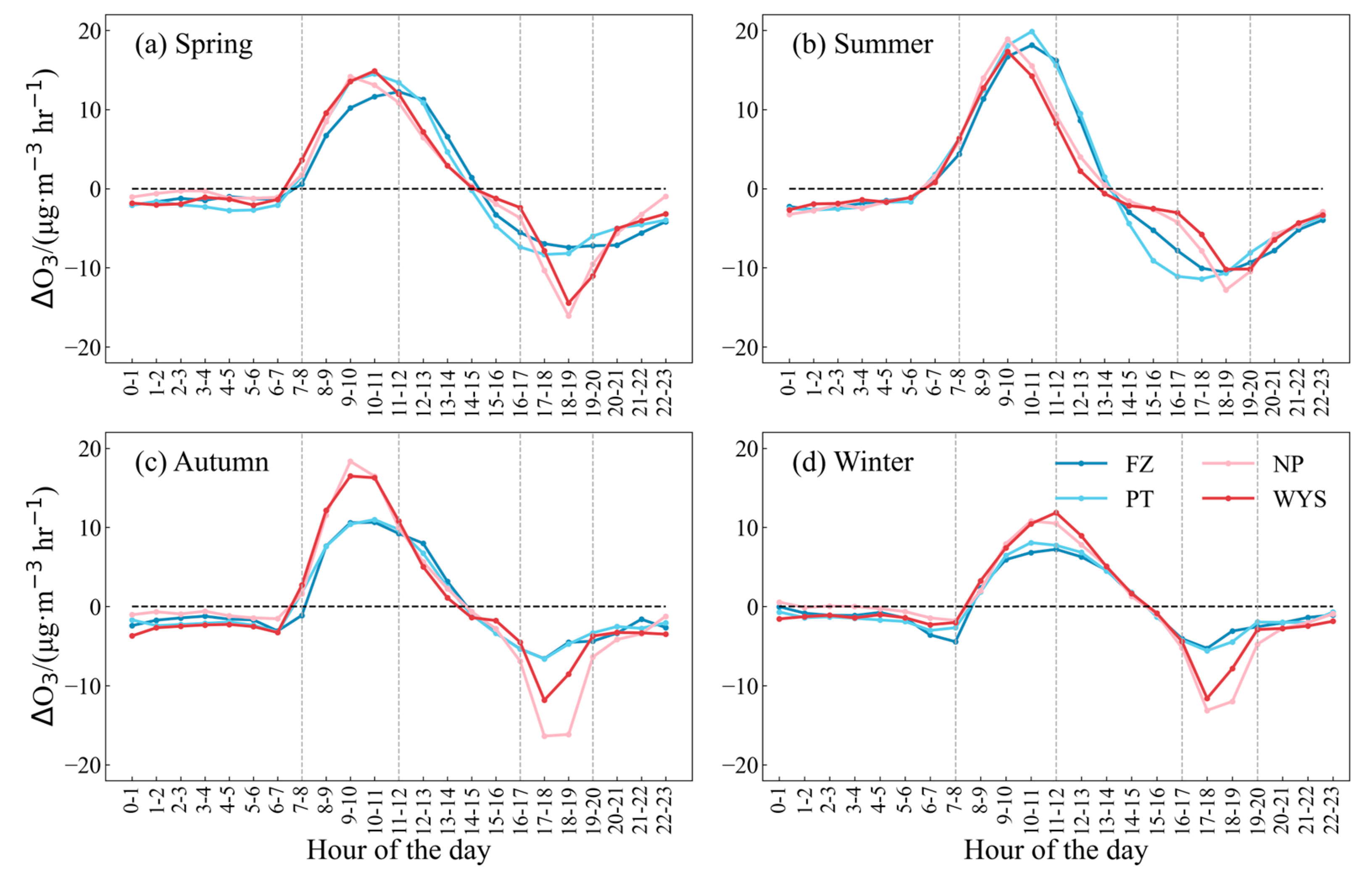
3.5. Diurnal Variability in Surface O3 Concentrations

Figure 11 shows the diurnal variation in O3 concentrations by season, averaged over 2016–2020 in the four areas. The diurnal variation is all characterized with a single-peak around 14:00–15:00 LST, and a minimum between 6:00–8:00 LST. Sunrise time and sunshine duration vary with season; so do the diurnal O3 concentrations in the four areas. The lowest O3 concentrations appear at 7:00 LST in both spring and autumn, at 6:00 LST in summer, and at 8:00 LST in winter. This pattern of diurnal variation is commonly observed elsewhere, reflecting net O3 production in daytime varying with solar radiation, and net O3 loss in nighttime due the O3 titration effect.
Nevertheless, differences are apparent among the four areas. First, the magnitude difference between the two inland areas is generally smaller than between the two coastal areas. The O3 level in Putian remains highest among the four areas. Second, the amplitude in diurnal variation is different among the areas. In spring, the amplitude of diurnal change between coastal and inland areas is similar, with a difference of about 3 μg·m−3. During summer, O3 production is primarily driven by photochemical reactions, leading to larger diurnal variations in O3 concentrations in the coastal areas than the inland areas. The daily variation amplitude reaches 81.1 μg·m−3 in the coastal areas, with a difference of 15.4 μg·m−3 compared to inland areas. In contrast, in autumn and winter, the inland areas exhibit larger diurnal variation amplitudes, with a maximum amplitude of 65.2 μg·m−3 in autumn when the amplitude for diurnal variation in the inland areas is 15.8 μg·m−3 higher than in the coastal areas.
We further examined the hourly change rate in O3 concentrations (ΔO3/Δh, where h is one hour) by taking the difference in O3 concentrations between two consecutive hours ( O 3 t O 3 t 1 ,   w h e r e   t = 2 , 3 , 4 . . . 24 , Figure 12). An interesting finding is that diurnal O3 change rate is generally similar between the two inland areas or between the two coastal areas, but different between the inland and coastal areas. Although the inland and coastal areas all show a peak during the midday and a valley near the sunset, there are two noticeable differences in spring, autumn, and winter. One is in the morning between 8:00–12:00 LST and the other between 17:00–20:00 LST. In the morning (8:00–12:00 LST), surface O3 concentrations increase faster in the inland areas than in the coast areas. The maximum difference in the O3 change rate is about 7 μg·m−3 h−1 in autumn. During 17:00–20:00 LST, O3 concentrations decrease faster in the inland areas than in the coastal areas, with the maximum difference in O3 decrease rate about 8 μg·m−3 h−1. However, in summer, the change rate of hourly O3 is different: O3 concentrations increase faster in the coastal areas than in the inland areas after 10:00 LST. In the meantime, O3 concentrations decrease more rapidly from 15:00 to 18:00 LST in the coastal areas than in the inland areas.
Because of the distinct sensitivity of O3 production to its precursors, O3 production can be categorized as “NOx-limited”, “VOCs-limited”, or in “transitional regimes” [56,57]. Within the NOx-limited regime, surface O3 formation rates increase significantly with NOx concentrations [58]. The sensitivity of O3 generation varies with space and time, both seasonally and diurnally [59,60,61]. For instance, due to differences in O3 precursor emissions between suburban and urban areas, O3 formation in urban areas is more sensitive to VOCs, whereas in suburban areas, it is more sensitive to NOx [62]. A previous study suggested that O3 production in inland areas is NOx-limited, while O3 production in coastal areas is VOCs-limited or in the transition zone [63]. During the morning peak traffic hours, NOx emissions increase and O3 concentrations in the inland areas are more sensitive to the increase of NOx and, thus, the O3 generation rate is higher in the inland areas than in the coastal areas. In addition, air temperature in the morning increases faster in the inland areas than in the coastal areas (Figure 13). As showed in Figure 4 and in the literature, higher temperature is conducive to the O3 photochemical production. Moreover, air in the morning becomes drier faster in the inland areas than in the coast areas (Figure 13), which hinders O3 dry deposition because leaf stomata tend to close under high VPD [50]. Overall, the combined effect of these chemical and meteorological conditions leads to a faster O3 increase rate in the morning in the inland areas than the coastal areas.
Over 17:00–20:00 LST in spring, autumn, and winter, O3 concentrations decrease at a faster rate in the inland areas than in the coastal areas, which is likely related to a stronger titration effect and a faster dry deposition rate of O3 in the inland areas. Figure 13 shows that during this period, NO2 concentrations increase faster in the inland areas than in the coastal areas, which coincides with the evening rush hour when NOx emissions increase while solar radiation decreases. During this time, NO titrates with O3, leading to the generation of NO2 and a decrease in O3 concentrations [64,65,66]. Therefore, the faster decline in O3 concentrations in the inland areas during this period is associated with the stronger titration effect in the inland areas. In addition, the change in O3 dry deposition during the period also play a role. As discussed, O3 dry deposition is largely modulated by leaf amount and leaf stomatal conductance. Over 17:00–20:00 LST, VPD in the inland areas decrease faster than in the coastal areas. In addition, LAI in the inland areas is larger than that in the coastal areas (Figure 3). These two factors favor consumption of more O3 through dry deposition. Therefore, the faster decline in O3 concentrations during 17:00–20:00 LST in the inland areas could be attractable to more O3 loss due to more NOx titration and lower deposition due to lower VPD, and more vegetation amount.
In summer, diurnal change rate of O3 concentrations is different from the other seasons. The rate in the coastal areas is similar to or higher than that in the inland areas over 8:00–14:00 LST, but lower than that over 14:00–18:00 LST. The reasons for the differences are unknown and thus call for further studies.

3.6. Seasonal Variability in Surface O3 Concentrations

Figure 14 shows the monthly variation in O3 concentrations. The difference among the four areas is still that O3 concentrations in the coastal areas are higher than in the inland areas throughout the year. The magnitude of O3 concentrations follows the order of Putian > Fuzhou > Nanping > Wuyishan. Putian is always with the highest O3 concentrations, with an annual mean MDA8 O3 concentrations of 100.5 μg·m−3 (Figure 10), which is closely related to its low level in vegetation cover, and high levels in emission levels, annual solar radiation, and temperature (Figure 3).
The seasonal variation in O3 concentrations is similar among all the areas, with a bimodal pattern of “high in spring and autumn, low in summer and winter”. This “M-shaped” seasonality is similar to that in the PRD, but different from that in the BTH and PRD [45,67], where an inverted “V-shaped” seasonality appears. The reasons for the M-shaped seasonality are suspected due to frequent typhoons and rainfall in summer [18].
We explore an explanation for the M-shaped seasonality from a different perspective. Through the GEOS-Chem tagged O3 simulation, we partitioned surface O3 into different components according to its sources. Figure 2 and Figure 15a show that GEOS-Chem can reasonably reproduce the M-shaped seasonality in the study areas. In Figure 15a, the local O3 source (net chemical production minus deposition) is indeed largest in summer, reducing gradually with solar radiation and temperature in the other seasons. However, inflow of O3 is transported from the rest of China, the rest of the world, and the stratosphere, which is high in spring and autumn, but low in summer and winter. The low inflow in winter is due to low net O3 production everywhere in the Northern Hemisphere, while the low inflow in summer is due to strong convection in southern China during the East Asian summer monsoon seasons, as showed in Han et al. and Chen et al. [19,68]. Non-local O3 usually is lifted in the its source regions, travelled in distance horizontally in the middle or upper troposphere, and then transported downward to the surface in the local areas. During the East Asian summer monsoon, local upward convection prevails in Fujian as shown in the peak of CAPE (Figure 15b). This prevents non-local O3 from reaching the surface. In addition, locally produced O3 is lifted upward [19]. Consequently, overall surface O3 becomes lower in summer.

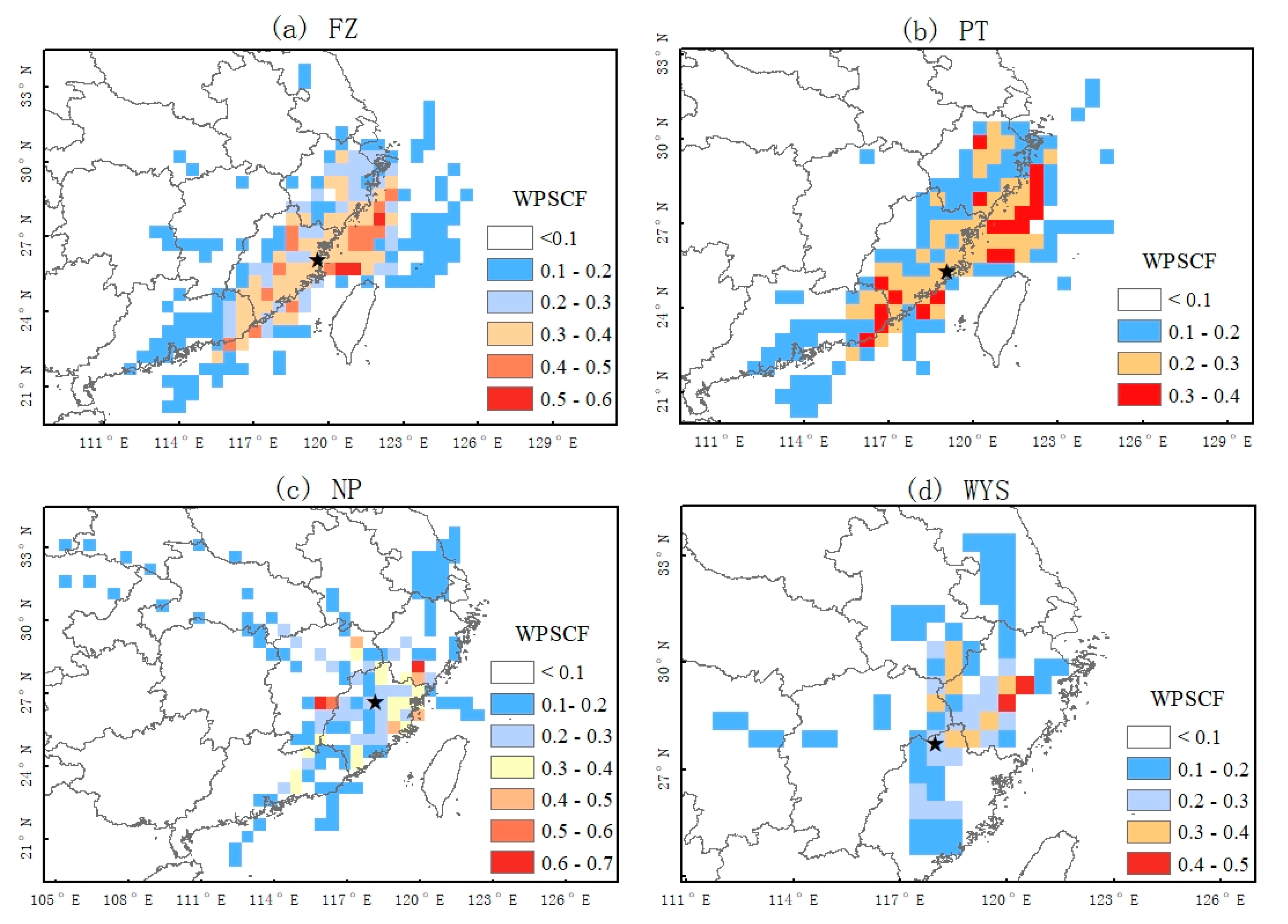
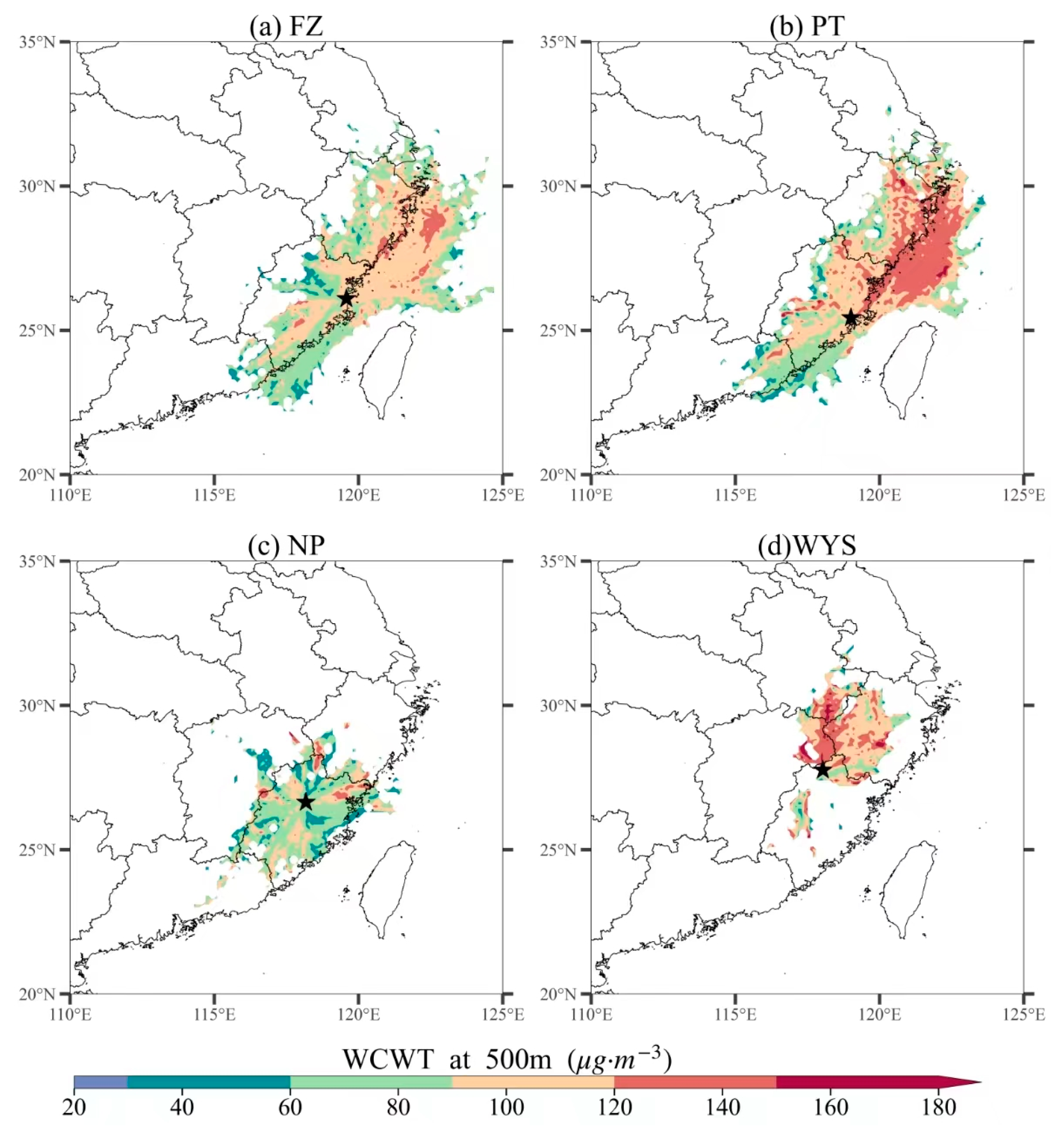
3.7. O3 Exceedance Days and Sources of O3 Identified by Trajectory Analysis

Table 2 shows the number of O3 exceedance days (MDA8 O3 > 160 μg·m−3) in the four areas based on the MDA8 O3 concentrations from 2016 to 2020. By year, there were more exceedance days in 2017 and 2018. By season, O3 exceedance episodes were least frequent in winter and mainly occurred in spring, summer, and fall. Spatially, coastal areas experienced a substantial higher number of exceedance days than inland areas. In total from 2016 to 2020, Putian experienced the highest number of exceedance days at 171, followed by Fuzhou at 166. In contrast, Nanping and Wuyishan, although with limited anthropogenic emissions, are not immune from O3 pollution, having experienced 51 and 29 exceedance days, respectively.
The source regions of O3 were identified by the WPSCF (Figure 16) and WCWT models (Figure 17). A higher WPSCF value in an area indicates that area having a higher probability as a O3 source area for O3 pollution in the receptor area, and a higher WCWT value means that area contributing more O3 to the receptor area.
Based on the WPSCF distribution derived from 24 h trajectories, the O3 source areas during O3 exceedance days for Fuzhou and Putian are similar. These areas mainly include the YRD, the coastal regions of Guangdong and Fujian provinces. The source areas for Nanping and Wuyishan in 24 h are mostly within Fujian province, partially from YRD, slightly from northwest or from west.
The WCWT distribution (Figure 17) is consistent with the WPSCP distribution (Figure 16). Within 24 h, high O3 in YRD is transported to Fuzhou and Putian, exacerbating O3 pollution in the areas. During O3 exceedance days, trajectories from the northeast and southwest flowing along the coast dominate the coastal areas. The YRD is the primary source region, and substantial O3 transport from the YRD region contributes largely to O3 pollution in Fuzhou and Putian.
In contrast, within 24 h, inland areas are mainly affected by O3 sources in smaller distances. During the exceedance days, Nanping is influenced by surrounding areas within the province, while in Wuyishan, the trajectories are predominantly from northeast in neighboring regions of Zhejiang and Jiangxi provinces.

4. Conclusions

In this study, we compared surface O3 concentrations between mountainous forest areas and urban areas in southeastern China. We selected two mountainous forest areas (Nanping and Wuyishan) and two lowland urban areas (Fuzhou and Putian) in Fujian province. Based on the geographical locations, we named the two types of areas as inland and coastal areas. By analyzing surface O3 observations from 2016 to 2020, we found that surface O3 variability in the two types of areas shares some similar features but also differs largely from diurnal to seasonal scales and on O3 exceedance days. We discussed the main driving factors for the similarities and differences, including O3 precursor emissions, meteorological conditions, and vegetation covers. Such a comprehensive comparison is rare in literature. The main conclusions are drawn as follows:
1. The mountainous forest areas (the inland areas) is characterized with limited human activates, low precursor emissions, humid and low air, and dense vegetation covers. This leads to low chemical O3 production and high O3 deposition rates. In contrast, the lowland urban areas (the coastal areas) are characterized with higher industrialization and population densities, higher levels of O3 precursor emissions, and lower vegetation covers, resulting in higher O3 concentrations at various time scales and more O3 exceedance days. The mean MDA8 O3 concentrations over 2016–2020 is 95.9 µg m−3 in the coastal areas, which is 15.4 µg m−3 (i.e. ~15%) higher than those in the inland areas (~80.5 µg m−3).
2. The day-to-day variation in surface O3 in the two types of the areas is rather similar, with a correlation coefficient of 0.75 between them, suggesting similar influences on large scales, such as weather patterns, regional O3 transport, and background O3. Over 2016–2020, O3 concentrations in all the areas shows a trend of “rising and then falling”, with a peak in 2017 and 2018. Daily variation in surface O3 is found to be highly correlated with daily meteorological conditions. Among all meteorological factors, the most influential ones include solar radiation for the coast areas and air humidity for the inland areas.
3. Diurnally, during the morning, O3 concentrations in the inland areas increase faster than in the coastal areas in most seasons, mainly due to faster increase in temperature and decrease in humidity. In contrast, O3 concentrations in the evening decrease faster in the inland areas than in the coastal areas, mostly attributable to higher titration effect in the inland areas.
4. Seasonally, both the areas share a “M-type” variation in O3 concentrations from January to December, with two peaks in spring and autumn and two valleys in summer and winter. We found this is caused by the summer Asian monsoon that induces large-scale convections in summer. Such convection transports local produced O3 to the upper layers while blocking non-local O3 from reaching the surface.
5. The coastal areas experienced a substantial higher number of exceedance days (~30 days per year) than inland areas (~5-10 days per year), largely due to regional transport of high O3 from the northeast, mainly the YRD region. The inland areas, although with limited anthropogenic emissions, are not immune from high O3 pollution, mainly occurring in spring and autumn.

Author Contributions

Conceptualization, X.C., X.J. and J.L.; methodology, X.J. and J.L.; software, X.J.; validation, X.C. and J.L.; formal analysis, M.Y., Z.C. (Zhiqiang Chen), X.C., J.L. and X.J.; investigation, Z.C. (Zhiqiang Chen) and C.G.; resources, Z.C. (Zhixiong Chen); data curation, Z.C. (Zhixiong Chen), J.H., H.D., H.W. and Y.J.; writing—original draft preparation, X.C., X.J. and J.L.; writing—review and editing, X.C. and J.L.; visualization, J.L.; supervision, X.C. and J.L.; project administration, J.L.; funding acquisition, X.C. and Z.C. (Zhiqiang Chen). All authors have read and agreed to the published version of the manuscript.

Funding

This study was supported by the National Natural Science Foundation of China (42275196), the Natural Science Foundation of Fujian Province (2021J01181), and the Public Welfare Special Projects for Research Institutes from Fujian Department of Science and Technology (2023R1014003, 2022R1002008).

Institutional Review Board Statement

Not applicable.

Informed Consent Statement

Not applicable.

Data Availability Statement

All datasets are publicly available except for ozone data in Wuyishan and observations from meteorological monitoring stations. All the data sources are described in the paper. Further inquiries can be directed to the corresponding author.

Acknowledgments

We thank China National Environmental Monitoring Station for the air quality data, Tsinghua University for the Multi-resolution Emission Inventory for China (MEIC) emission inventory, University of Maryland for the LAI data from the GLASS product, the European Weather Prediction Centre for the ERA5 reanalysis meteorological data and Fujian Meteorological Bureau for the meteorological observation data. We are grateful to Fujian Normal University for providing computing resources.

Conflicts of Interest

The authors declare no conflicts of interest.

References

  1. Song, M.; Li, X.; Yang, S.; Yu, X.; Zhou, S.; Yang, Y.; Chen, S.; Dong, H.; Liao, K.; Chen, Q.; et al. Spatiotemporal variation, sources, and secondary transformation potential of volatile organic compounds in Xi’an, China. Atmos. Chem. Phys. 2021, 21, 4939–4958. [Google Scholar] [CrossRef]
  2. Haagen-Smit, A.J. Chemistry and Physiology of Los Angeles Smog. Ind. Eng. Chem. 1952, 44, 1342–1346. [Google Scholar] [CrossRef]
  3. Wang, S.; Zhao, Y.; Han, Y.; Li, R.; Fu, H.; Gao, S.; Duan, Y.; Zhang, L.; Chen, J. Spatiotemporal variation, source and secondary transformation potential of volatile organic compounds (VOCs) during the winter days in Shanghai, China. Atmos. Environ. 2022, 286, 119203. [Google Scholar] [CrossRef]
  4. Zhao, D.D.; Xin, J.Y.; Wang, W.F.; Jia, D.J.; Wang, Z.F.; Xiao, H.; Liu, C.; Zhou, J.; Tong, L.; Ma, Y.J.; et al. Effects of the sea-land breeze on coastal ozone pollution in the Yangtze River Delta, China. Sci. Total Environ. 2022, 807, 150306. [Google Scholar] [CrossRef] [PubMed]
  5. Zeng, Y.; Cao, Y.; Qiao, X.; Seyler, B.C.; Tang, Y. Air pollution reduction in China: Recent success but great challenge for the future. Sci. Total Environ. 2019, 663, 329–337. [Google Scholar] [CrossRef] [PubMed]
  6. Pan, S.; Roy, A.; Choi, Y.; Eslami, E.; Thomas, S.; Jiang, X.; Gao, H.O. Potential impacts of electric vehicles on air quality and health endpoints in the Greater Houston Area in 2040. Atmos. Environ. 2019, 207, 38–51. [Google Scholar] [CrossRef]
  7. Mills, G.; Pleijel, H.; Malley, C.S.; Sinha, B.; Cooper, O.R.; Schultz, M.G.; Neufeld, H.S.; Simpson, D.; Sharps, K.; Feng, Z.; et al. Tropospheric Ozone Assessment Report: Present-day tropospheric ozone distribution and trends relevant to vegetation. Elem. Sci. Anthr. 2018, 6, 47. [Google Scholar] [CrossRef]
  8. Wang, T.; Xue, L.; Feng, Z.; Dai, J.; Zhang, Y.; Tan, Y. Ground-level ozone pollution in China: A synthesis of recent findings on influencing factors and impacts. Environ. Res. Lett. 2022, 17, 063003. [Google Scholar] [CrossRef]
  9. Lu, X.; Zhang, L.; Wang, X.; Gao, M.; Li, K.; Zhang, Y.; Yue, X.; Zhang, Y. Rapid increases in warm-season surface ozone and resulting health impact in China since 2013. Environ. Sci. Technol. Lett. 2020, 7, 240–247. [Google Scholar] [CrossRef]
  10. Liu, Y.; Wang, T. Worsening urban ozone pollution in China from 2013 to 2017—Part 1: The complex and varying roles of meteorology. Atmos. Chem. Phys. 2020, 20, 6305–6321. [Google Scholar] [CrossRef]
  11. Wang, Z.; Lv, J.; Tan, Y.; Guo, M.; Gu, Y.; Xu, S.; Zhou, Y. Temporospatial variations and Spearman correlation analysis of ozone concentrations to nitrogen dioxide, sulfur dioxide, particulate matters and carbon monoxide in ambient air, China. Atmos. Pollut. Res. 2019, 10, 1203–1210. [Google Scholar] [CrossRef]
  12. Li, K.; Jacob, D.J.; Liao, H.; Shen, L.; Zhang, Q.; Bates, K.H. Anthropogenic drivers of 2013–2017 trends in summer surface ozone in China. Proc. Natl. Acad. Sci. USA 2019, 116, 422–427. [Google Scholar] [CrossRef]
  13. Gong, C.; Liao, H.; Zhang, L.; Yue, X.; Dang, R.; Yang, Y. Persistent ozone pollution episodes in North China exacerbated by regional transport. Environ. Pollut. 2020, 265, 115056. [Google Scholar] [CrossRef]
  14. Zhang, Y.; Yu, S.; Chen, X.; Li, Z.; Li, M.; Song, Z.; Liu, W.; Li, P.; Zhang, X.; Lichtfouse, E.; et al. Local production, downward and regional transport aggravated surface ozone pollution during the historical orange-alert large-scale ozone episode in eastern China. Environ. Chem. Lett. 2022, 20, 1577–1588. [Google Scholar] [CrossRef]
  15. Mao, J.; Tai, A.P.K.; Yung, D.H.Y.; Yuan, T.; Chau, K.T.; Feng, Z. Multidecadal ozone trends in China and implications for human health and crop yields: A hybrid approach combining chemical transport model and machine learning. EGUsphere 2023, 2023, 1–25. [Google Scholar] [CrossRef]
  16. Liu, Y.; Geng, G.; Cheng, J.; Liu, Y.; Xiao, Q.; Liu, L.; Shi, Q.; Tong, D.; He, K.; Zhang, Q. Drivers of Increasing Ozone during the Two Phases of Clean Air Actions in China 2013–2020. Environ. Sci. Technol. 2023, 57, 8954–8964. [Google Scholar] [CrossRef]
  17. Ji, X.; Hong, Y.; Lin, Y.; Xu, K.; Chen, G.; Liu, T.; Xu, L.; Li, M.; Fan, X.; Wang, H.; et al. Impacts of synoptic patterns and meteorological factors on distribution trends of ozone in southeast China during 2015–2020. J. Geophys. Res. Atmos. 2023, 128, e2022JD037961. [Google Scholar] [CrossRef]
  18. Ge, C.; Liu, J.; Cheng, X.; Fang, K.; Chen, Z.; Chen, Z.; Hu, J.; Jiang, D.; Shen, L.; Yang, M. Impact of regional transport on high ozone episodes in southeast coastal regions of China. Atmos. Pollut. Res. 2022, 13, 101497. [Google Scholar] [CrossRef]
  19. Chen, Z.; Xie, Y.; Liu, J.; Shen, L.; Cheng, X.; Han, H.; Yang, M.; Shen, Y.; Zhao, T.; Hu, J. Distinct seasonality in vertical variations of tropospheric ozone over coastal regions of southern China. Sci. Total Environ. 2023, 874, 162423. [Google Scholar] [CrossRef]
  20. Chen, G.; Liu, T.; Chen, J.; Xu, L.; Hu, B.; Yang, C.; Fan, X.; Li, M.; Hong, Y.; Ji, X.; et al. Atmospheric oxidation capacity and O3 formation in a coastal city of southeast China: Results from simulation based on four-season observation. J. Environ. Sci. 2024, 136, 68–80. [Google Scholar] [CrossRef]
  21. Zhang, X.; Wu, Z.; He, Z.; Zhong, X.; Bi, F.; Li, Y.; Gao, R.; Li, H.; Wang, W. Spatiotemporal patterns and ozone sensitivity of gaseous carbonyls at eleven urban sites in southeastern China. Sci. Total Environ. 2022, 824, 153719. [Google Scholar] [CrossRef] [PubMed]
  22. Hong, Z.; Li, M.; Wang, H.; Xu, L.; Hong, Y.; Chen, J.; Chen, J.; Zhang, H.; Zhang, Y.; Wu, X.; et al. Characteristics of atmospheric volatile organic compounds (VOCs) at a mountainous forest site and two urban sites in the southeast of China. Sci. Total Environ. 2019, 657, 1491–1500. [Google Scholar] [CrossRef] [PubMed]
  23. Ji, X.; Chen, G.; Chen, J.; Xu, L.; Lin, Z.; Zhang, K.; Fan, X.; Li, M.; Zhang, F.; Wang, H.; et al. Meteorological impacts on the unexpected ozone pollution in coastal cities of China during the unprecedented hot summer of 2022. Sci. Total Environ. 2024, 914, 170035. [Google Scholar] [CrossRef] [PubMed]
  24. Chen, G.; Shi, Q.; Xu, L.; Yu, S.; Lin, Z.; Ji, X.; Fan, X.; Hong, Y.; Li, M.; Zhang, F.; et al. Photochemistry in the urban agglomeration along the coastline of southeastern China: Pollution mechanism and control implication. Sci. Total Environ. 2023, 901, 166318. [Google Scholar] [CrossRef]
  25. Lin, C.; Zhang, W. Using a Pollution-to-Risk Method to Evaluate the Impact of a Cold Front: A Case Study in a Downstream Region in Southeastern China. Atmosphere 2022, 13, 1944. [Google Scholar] [CrossRef]
  26. Kan, H.D. A review of standard value of fine particulate matter (PM(2.5)) ruled by National Ambient Air Quality Standards (GB3095-2012) in China. Chin. J. Preventive Med. 2012, 46, 396–398. [Google Scholar]
  27. Liu, X.H.; Zhu, B.; Zhu, T.; Liao, H. The Seesaw Pattern of PM2.5 Interannual Anomalies Between Beijing-Tianjin-Hebei and Yangtze River Delta Across Eastern China in Winter. Geophys. Res. Lett. 2022, 49, e2021GL095878. [Google Scholar] [CrossRef]
  28. Hua, W.; Wu, B. Atmospheric circulation anomaly over mid- and high-latitudes and its association with severe persistent haze events in Beijing. Atmos. Res. 2022, 277, 106315. [Google Scholar] [CrossRef]
  29. Breiman, L. Random Forests. Mach. Learn. 2001, 45, 5–32. [Google Scholar] [CrossRef]
  30. Biau, G. Analysis of a Random Forests Model. J. Mach. Learn. Res. 2010, 13, 1063–1095. [Google Scholar]
  31. Dietterich, T.G. An Experimental Comparison of Three Methods for Constructing Ensembles of Decision Trees: Bagging, Boosting, and Randomization. Mach. Learn. 2000, 40, 139–157. [Google Scholar] [CrossRef]
  32. Xiong, K.; Xie, X.; Mao, J.; Wang, K.; Huang, L.; Li, J.; Hu, J. Improving the accuracy of O3 prediction from a chemical transport model with a random forest model in the Yangtze River Delta region, China. Environ. Pollut. 2023, 319, 120926. [Google Scholar] [CrossRef] [PubMed]
  33. Li, T.; Lu, Y.; Deng, X.; Zhan, Y. Spatiotemporal variations in meteorological influences on ambient ozone in China: A machine learning approach. Atmos. Pollut. Res. 2023, 14, 101720. [Google Scholar] [CrossRef]
  34. Zhan, Y.; Luo, Y.; Deng, X.; Grieneisen, M.L.; Zhang, M.; Di, B. Spatiotemporal prediction of daily ambient ozone levels across China using random forest for human exposure assessment. Environ. Pollut. 2018, 233, 464–473. [Google Scholar] [CrossRef] [PubMed]
  35. Bey, I.; Jacob, D.J.; Yantosca, R.M.; Logan, J.A.; Field, B.D.; Fiore, A.M.; Li, Q.; Liu, H.Y.; Mickley, L.J.; Schultz, M.G. Global modeling of tropospheric chemistry with assimilated meteorology: Model description and evaluation. J. Geophys. Res. Atmos. 2001, 106, 23073–23095. [Google Scholar] [CrossRef]
  36. Keller, C.A.; Long, M.S.; Yantosca, R.M.; Da Silva, A.M.; Pawson, S.; Jacob, D.J. HEMCO v1.0: A versatile, ESMF-compliant component for calculating emissions in atmospheric models. Geosci. Model Dev. 2014, 7, 1409–1417. [Google Scholar] [CrossRef]
  37. Guenther, A.B.; Jiang, X.; Heald, C.L.; Sakulyanontvittaya, T.; Duhl, T.; Emmons, L.K.; Wang, X. The Model of Emissions of Gases and Aerosols from Nature version 2.1 (MEGAN2.1): An extended and updated framework for modeling biogenic emissions. Geosci. Model Dev. 2012, 5, 1471–1492. [Google Scholar] [CrossRef]
  38. Hudman, R.C.; Moore, N.E.; Mebust, A.K.; Martin, R.V.; Russell, A.R.; Valin, L.C.; Cohen, R.C. Steps towards a mechanistic model of global soil nitric oxide emissions: Implementation and space based-constraints. Atmos. Chem. Phys. 2012, 12, 7779–7795. [Google Scholar] [CrossRef]
  39. Hoesly, R.M.; Smith, S.J.; Feng, L.; Klimont, Z.; Janssens-Maenhout, G.; Pitkanen, T.; Seibert, J.J.; Vu, L.; Andres, R.J.; Bolt, R.M.; et al. Historical (1750–2014) anthropogenic emissions of reactive gases and aerosols from the Community Emissions Data System (CEDS). Geosci. Model Dev. 2018, 11, 369–408. [Google Scholar] [CrossRef]
  40. Gong, C.; Liao, H. A typical weather pattern for ozone pollution events in North China. Atmos. Chem. Phys. 2019, 19, 13725–13740. [Google Scholar] [CrossRef]
  41. Zhou, X.; Li, Z.; Zhang, T.; Wang, F.; Wang, F.; Tao, Y.; Zhang, X.; Wang, F.; Huang, J. Volatile organic compounds in a typical petrochemical industrialized valley city of northwest China based on high-resolution PTR-MS measurements: Characterization, sources and chemical effects. Sci. Total Environ. 2019, 671, 883–896. [Google Scholar] [CrossRef] [PubMed]
  42. Zheng, H.; Kong, S.; Xing, X.; Mao, Y.; Hu, T.; Ding, Y.; Li, G.; Liu, D.; Li, S.; Qi, S. Monitoring of volatile organic compounds (VOCs) from an oil and gas station in northwest China for 1 year. Atmos. Chem. Phys. 2018, 18, 4567–4595. [Google Scholar] [CrossRef]
  43. Liu, B.; Cheng, Y.; Zhou, M.; Liang, D.; Dai, Q.; Wang, L.; Jin, W.; Zhang, L.; Ren, Y.; Zhou, J.; et al. Effectiveness evaluation of temporary emission control action in 2016 in winter in Shijiazhuang, China. Atmos. Chem. Phys. 2018, 18, 7019–7039. [Google Scholar] [CrossRef]
  44. Ren, B.; Xie, P.; Xu, J.; Li, A.; Tian, X.; Hu, Z.; Huang, Y.; Li, X.; Zhang, Q.; Ren, H.; et al. Use of the PSCF method to analyze the variations of potential sources and transports of NO2, SO2, and HCHO observed by MAX-DOAS in Nanjing, China during 2019. Sci. Total Environ. 2021, 782, 146865. [Google Scholar] [CrossRef]
  45. Han, H.; Liu, J.E.; Shu, L.; Wang, T.J.; Yuan, H.L. Local and synoptic meteorological influences on daily variability in summertime surface ozone in eastern China. Atmos. Chem. Phys. 2020, 20, 203–222. [Google Scholar] [CrossRef]
  46. Wang, T.; Xue, L.; Brimblecombe, P.; Lam, Y.F.; Li, L.; Zhang, L. Ozone pollution in China: A review of concentrations, meteorological influences, chemical precursors, and effects. Sci. Total Environ. 2017, 575, 1582–1596. [Google Scholar] [CrossRef] [PubMed]
  47. Cheng, X.; Liu, J.; Zhao, T.; Gong, S.; Xu, X.; Xie, X.; Wang, R. A teleconnection between sea surface temperature in the central and eastern Pacific and wintertime haze variations in southern China. Theor. Appl. Climatol. 2021, 143, 349–359. [Google Scholar] [CrossRef]
  48. Zhang, L.; Brook, J.R.; Vet, R. A revised parameterization for gaseous dry deposition in air-quality models. Atmos. Chem. Phys. 2003, 3, 2067–2082. [Google Scholar] [CrossRef]
  49. Yin, Z.; Cao, B.; Wang, H. Dominant patterns of summer ozone pollution in eastern China and associated atmospheric circulations. Atmos. Chem. Phys. 2019, 19, 13933–13943. [Google Scholar] [CrossRef]
  50. Kavassalis, S.C.; Murphy, J.G. Understanding ozone-meteorology correlations: A role for dry deposition. Geophys. Res. Lett. 2017, 44, 2922–2931. [Google Scholar] [CrossRef]
  51. He, J.J.; Gong, S.L.; Yu, Y.; Yu, L.J.; Wu, L.; Mao, H.J.; Song, C.B.; Zhao, S.P.; Liu, H.L.; Li, X.Y.; et al. Air pollution characteristics and their relation to meteorological conditions during 2014–2015 in major Chinese cities. Environ. Pollut. 2017, 223, 484–496. [Google Scholar] [CrossRef] [PubMed]
  52. Yang, Y.; Zhou, Y.; Wang, H.; Li, M.; Li, H.; Wang, P.; Yue, X.; Li, K.; Zhu, J.; Liao, H. Meteorological characteristics of extreme ozone pollution events in China and their future predictions. Atmos. Chem. Phys. 2024, 24, 1177–1191. [Google Scholar] [CrossRef]
  53. Chen, Z.; Li, R.; Chen, D.; Zhuang, Y.; Gao, B.; Yang, L.; Li, M. Understanding the causal influence of major meteorological factors on ground ozone concentrations across China. J. Clean. Prod. 2020, 242, 118498. [Google Scholar] [CrossRef]
  54. Sun, L.; Xue, L.; Wang, Y.; Li, L.; Lin, J.; Ni, R.; Yan, Y.; Chen, L.; Li, J.; Zhang, Q.; et al. Impacts of meteorology and emissions on summertime surface ozone increases over central eastern China between 2003 and 2015. Atmos. Chem. Phys. 2019, 19, 1455–1469. [Google Scholar] [CrossRef]
  55. Hu, C.; Kang, P.; Jaffe, D.A.; Li, C.; Zhang, X.; Wu, K.; Zhou, M. Understanding the impact of meteorology on ozone in 334 cities of China. Atmos. Environ. 2021, 248, 118221. [Google Scholar] [CrossRef]
  56. Chu, W.; Li, H.; Ji, Y.; Zhang, X.; Xue, L.; Gao, J.; An, C. Research on ozone formation sensitivity based on observational methods: Development history, methodology, and application and prospects in China. J. Environ. Sci. 2024, 138, 543–560. [Google Scholar] [CrossRef]
  57. Lu, H.; Lyu, X.; Cheng, H.; Ling, Z.; Guo, H. Overview on the spatial-temporal characteristics of the ozone formation regime in China. Environmental science. Processes & impacts. 2019, 21, 916–929. [Google Scholar]
  58. Yang, L.; Yuan, Z.; Luo, H.; Wang, Y.; Xu, Y.; Duan, Y.; Fu, Q. Identification of long-term evolution of ozone sensitivity to precursors based on two-dimensional mutual verification. Sci. Total Environ. 2021, 760, 143401. [Google Scholar] [CrossRef]
  59. Wang, W.; van der A, R.; Ding, J.; van Weele, M.; Cheng, T. Spatial and temporal changes of the ozone sensitivity in China based on satellite and ground-based observations. Atmos. Chem. Phys. 2021, 21, 7253–7269. [Google Scholar] [CrossRef]
  60. Vermeuel, M.P.; Novak, G.A.; Alwe, H.D.; Hughes, D.D.; Kaleel, R.; Dickens, A.F.; Kenski, D.; Czarnetzki, A.C.; Stone, E.A.; Stanier, C.O.; et al. Sensitivity of ozone production to NOx and VOC along the Lake Michigan coastline. J. Geophys. Res. Atmos. 2019, 124, 10989–11006. [Google Scholar] [CrossRef]
  61. Orlando, J.P.; Alvim, D.S.; Yamazaki, A.; Corrêa, S.M.; Gatti, L.V. Ozone precursors for the São Paulo Metropolitan Area. Sci. Total Environ. 2010, 408, 1612–1620. [Google Scholar] [CrossRef] [PubMed]
  62. Cheng, N.; Li, R.; Xu, C.; Chen, Z.; Chen, D.; Meng, F.; Cheng, B.; Ma, Z.; Zhuang, Y.; He, B.; et al. Ground ozone variations at an urban and a rural station in Beijing from 2006 to 2017: Trend, meteorological influences and formation regimes. J. Clean. Prod. 2019, 235, 11–20. [Google Scholar] [CrossRef]
  63. Zhang, H.; Wang, Y.; Lu, Y.; Wang, Y.; Yu, C.; Wang, J.; Cao, D.; Jiang, H. Identification of ozone pollution control zones and types in China. China Environ. Sci. 2021, 41, 4051–4059. [Google Scholar]
  64. Nguyen, D.-H.; Lin, C.; Vu, C.-T.; Cheruiyot, N.K.; Nguyen, M.K.; Le, T.H.; Lukkhasorn, W.; Vo, T.-D.-H.; Bui, X.-T. Tropospheric ozone and NOx: A review of worldwide variation and meteorological influences. Environ. Technol. Innov. 2022, 28, 102809. [Google Scholar] [CrossRef]
  65. Tan, Z.; Lu, K.; Dong, H.; Hu, M.; Li, X.; Liu, Y.; Lu, S.; Shao, M.; Su, R.; Wang, H.; et al. Explicit diagnosis of the local ozone production rate and the ozone-NOx-VOC sensitivities. Sci. Bull. 2018, 63, 1067–1076. [Google Scholar] [CrossRef] [PubMed]
  66. Hu, X.M.; Doughty, D.C.; Sanchez, K.J.; Joseph, E.; Fuentes, J.D. Ozone variability in the atmospheric boundary layer in Maryland and its implications for vertical transport model. Atmos. Environ. 2012, 46, 354–364. [Google Scholar] [CrossRef]
  67. Liu, N.; Lin, W.; Ma, J.; Xu, W.; Xu, X. Seasonal variation in surface ozone and its regional characteristics at global atmosphere watch stations in China. J. Environ. Sci. 2019, 77, 291–302. [Google Scholar] [CrossRef]
  68. Han, H.; Liu, J.; Yuan, H.; Wang, T.; Zhuang, B.; Zhang, X. Foreign influences on tropospheric ozone over East Asia through global atmospheric transport. Atmos. Chem. Phys. 2019, 19, 12495–12514. [Google Scholar] [CrossRef]
Figure 1. Locations of the four areas of interest and corresponding air quality monitoring stations, which are overlaid with topography. Inland and coastal stations are indicated in red and blue dots, respectively.
Atmosphere 15 00519 g001
Figure 2. Comparison between observed (blue line) and GEOS-Chem simulated (orange line) MDA8 O3 concentrations in the four areas.
Atmosphere 15 00519 g002
Figure 3. The GDP, population, O3 precursor emissions (VOC, NOx, and CO), meteorological conditions (radiation: R, air temperature: T, relative humidity: R, and precipitation: Rain), leaf area index (LAI), and elevation. All values are the means over 2016–2020. Sources: Meteorological data (ad) are from the Fujian Meteorological Bureau. The emissions data (eg) are from the Multi-Resolution Emission Inventory for China (MEIC) emission inventory of Tsinghua University (http://meicmodel.org.cn, accessed on 10 January 2024). LAI data (h) are from GLASS data from the University of Maryland (http://glass.umd.edu, accessed on 6 July 2023). The elevation data (i) are from the Geospatial Data Cloud (https://www.gscloud.cn/search, accessed on 10 January 2023). Population and GDP data (j,k) are from Fujian Provincial Bureau of Statistics (https://tjj.fujian.gov.cn/tjgg/, accessed on 15 January 2023).
Atmosphere 15 00519 g003
Figure 4. (a) Daily MDA8 O3 time series from 2016 to 2020, with inland areas in reddish colors and coastal areas in bluish color. The multiple-year mean MDA8 O3 concentrations for the coastal and inland areas are indicated by dashed blue and red line and text, respectively. The national standard for O3 exceedance days, i.e., 160 µg m−3, is denoted with a grey dashed line. (b) The same as (a), but for the 11-day running average. The correlation coefficient of the time series between the inland and coastal areas, between coastal areas, and between inland areas are indicated in text.
Atmosphere 15 00519 g004
Figure 5. Comparisons of GEOS-Chem simulated seasonal variations in net chemical production (a) and deposition (b) in the four areas.
Atmosphere 15 00519 g005
Figure 6. Daytime (a1a4) and nighttime (b1b4) surface O3 and corresponding surface air temperature and relative humidity variations.
Atmosphere 15 00519 g006
Figure 7. O3 concentration versus wind speed and direction in the four areas.
Atmosphere 15 00519 g007
Figure 8. The correlation between daily meteorological factors and MDA8 O3 in each area in annual mean and by season. All the correlations are significant at a 99% level except the indicated.
Atmosphere 15 00519 g008
Figure 9. Comparison between observed and predicted MDA8 O3 in the four areas from 2016 to 2020.
Atmosphere 15 00519 g009
Figure 10. Importance ranking of RF model variables in the four areas, 2016 to 2020.
Atmosphere 15 00519 g010
Figure 11. Diurnal variation of O3 concentrations in the four areas by season from 2016 to 2020.
Atmosphere 15 00519 g011
Figure 12. The mean (2016–2022) diurnal hourly O3 change in the four areas by season.
Atmosphere 15 00519 g012
Figure 13. The mean (2016–2022) hourly change rates in NO2, temperature, and VPD during the indicated hours of the day in the inland and coastal areas in spring, autumn, and winter.
Atmosphere 15 00519 g013
Figure 14. Seasonal variations in MDA8 O3 concentrations for the coastal and inland areas. All the values are the means over 2016–2020.
Atmosphere 15 00519 g014
Figure 15. (a) GEOS-Chem simulated seasonal variations and associated components by source region. FJ indicates the local O3 source, ROC, O3 from the rest of China, ROW, O3 from the rest of the world, and Strat, O3 from the stratosphere. (b) The monthly mean convective available potential energy (CAPE) in Fujian (unit: J kg−1).
Atmosphere 15 00519 g015
Figure 16. WPSCT distribution for the receptor areas: Fujian (a), Putian (b), Nanping (c), and Wuyishan (d). The grey lines enclose provincial boundaries. The black star represents the location of each receptor area.
Atmosphere 15 00519 g016
Figure 17. WCWT distribution for the receptor areas: Fujian (a), Putian (b), Nanping (c), and Wuyishan (d). The grey lines enclose provincial boundaries. The black star represents the location of each receptor area.
Atmosphere 15 00519 g017
Table 1. Geo-information on air quality monitoring stations and weather stations in the four studied areas.
AreaMonitoring StationsLongitudeLatitudeElevation/(m)
Fuzhou
(FZ)
Kuaian119.41° E26.02° N6
Shida119.30° E26.03° N22
Wusibeilu119.29° E26.10° N4
Yangqiaoxilu119.26° E26.07° N11
Ziyang119.31° E26.07° N10
Jiulong119.58° E26.09° N10
Meteorological station119.28° E26.08° N84
Putian
(PT)
Lichengqucanghoulu119.01° E25.44° N18
Putian monitoring station119.00° E25.45° N21
Hanjiangquliuzhong119.11° E25.45° N14
Xiuyuquzhengfu119.10° E25.32° N17
Meteorological station119.00° E25.45° N81
Nanping
(NP)
Nanping monitoring stations118.16° E26.63° N96
Lvyeyouxianggongsi118.18° E26.65° N111
Qizhong118.17° E26.62° N112
Meteorological station118.17° E26.65° N152
Wuyishan
(WYS)
Yizhong118.03° E27.76° N223
Wuyixueyuan117.80° E27.73° N222
Meteorological station118.02° E27.76° N222
Table 2. O3 exceedance days in the four areas by year and by season.
YearFZPTNPWYSSeasonFZPTNPWYS
2016272163Spring6362265
20174453297Summer545564
20184852811Autumn46501220
2019202136Winter3470
2020272452Total1661715129
Total1661715129
Mean33.234.210.25.8
Disclaimer/Publisher’s Note: The statements, opinions and data contained in all publications are solely those of the individual author(s) and contributor(s) and not of MDPI and/or the editor(s). MDPI and/or the editor(s) disclaim responsibility for any injury to people or property resulting from any ideas, methods, instructions or products referred to in the content.

